1

Practical Implementation of Optimal Operation using Off-Line Computations

Sigurd Skogestad

Department of Chemical Engineering

Norwegian University of Science and Tecnology (NTNU)

Trondheim, Norway

5

Research Sigurd Skogestad

1. Truls Larsson, Studies on plantwide control, Aug. 2000. (Aker Kværner, Stavanger) 2. Eva-Katrine Hilmen, Separation of azeotropic mixtures, Des. 2000. (ABB, Oslo) 3. Ivar J. Halvorsen; Minimum energy requirements in distillation ,May 2001. (SINTEF) 4. Marius S. Govatsmark, Integrated optimization and control, Sept. 2003. (Statoil, Haugesund) 5. Audun Faanes, Controllability analysis and control structures, Sept. 2003. (Statoil, Trondheim) 6. Hilde K. Engelien, Process integration for distillation columns, March 2004. (Aker Kværner) 7. Stathis Skouras, Heteroazeotropic batch distillation, May 2004. (StatoilHydro, Haugesund) 8. Vidar Alstad, Studies on selection of controlled variables, June 2005. (Statoil, Porsgrunn) 9. Espen Storkaas, Control solutions to avoid slug flow in pipeline-riser systems, June 2005. (ABB) 10. Antonio C.B. Araujo, Studies on plantwide control, Jan. 2007. (Un. Campina Grande, Brazil) 11. Tore Lid, Data reconciliation and optimal operation of refinery processes , June 2007 (Statoil)12. Federico Zenith, Control of fuel cells, June 2007 (Max Planck Institute, Magdeburg) 13. Jørgen B. Jensen, Optimal operation of refrigeration cycles, May 2008 (ABB, Oslo) 14. Heidi Sivertsen, Stabilization of desired flow regimes (no slug), Dec. 2008 (Statoil, Stjørdal) 15. Elvira M.B. Aske, Plantwide control systems with focus on max throughput, Mar 2009 (Statoil)16. Andreas Linhart An aggregation model reduction method for one-dimensional distributed

systems, Oct. 2009.

Current research:• Restricted-complexity control (self-optimizing control):

• off-line and analytical solutions to optimal control (incl. explicit MPC & explicit RTO)•Henrik Manum, Johannes Jäschke, Håkon Dahl-Olsen, Ramprasad Yelshuru

•Plantwide control. Applications: LNG, GTL•Magnus G. Jacobsen, Mehdi Panahi,

Graduated PhDs since 2000

6

Outline

• Implementation of optimal operation

• Paradigm 1: On-line optimizing control

• Paradigm 2: "Self-optimizing" control schemes– Precomputed (off-line) solution

• Examples

• Control of optimal measurement combinations– Nullspace method

– Exact local method

– Link to optimal control / Explicit MPC

• Conclusion

8

Optimal operation

• A typical dynamic optimization problem

• Implementation: “Open-loop” solutions not robust to disturbances or model errors

• Want to introduce feedback

9

Implementation of optimal operation

• Paradigm 1: On-line optimizing control where measurements are used to update model and states

• Paradigm 2: “Self-optimizing” control scheme found by exploiting properties of the solution

10

Implementation: Paradigm 1

• Paradigm 1: Online optimizing control

• Measurements are primarily used to update the model

• The optimization problem is resolved online to compute new inputs.

• Example: Conventional MPC, RTO (real-time optimization)

• This is the “obvious” approach (for someone who does not know control)

12

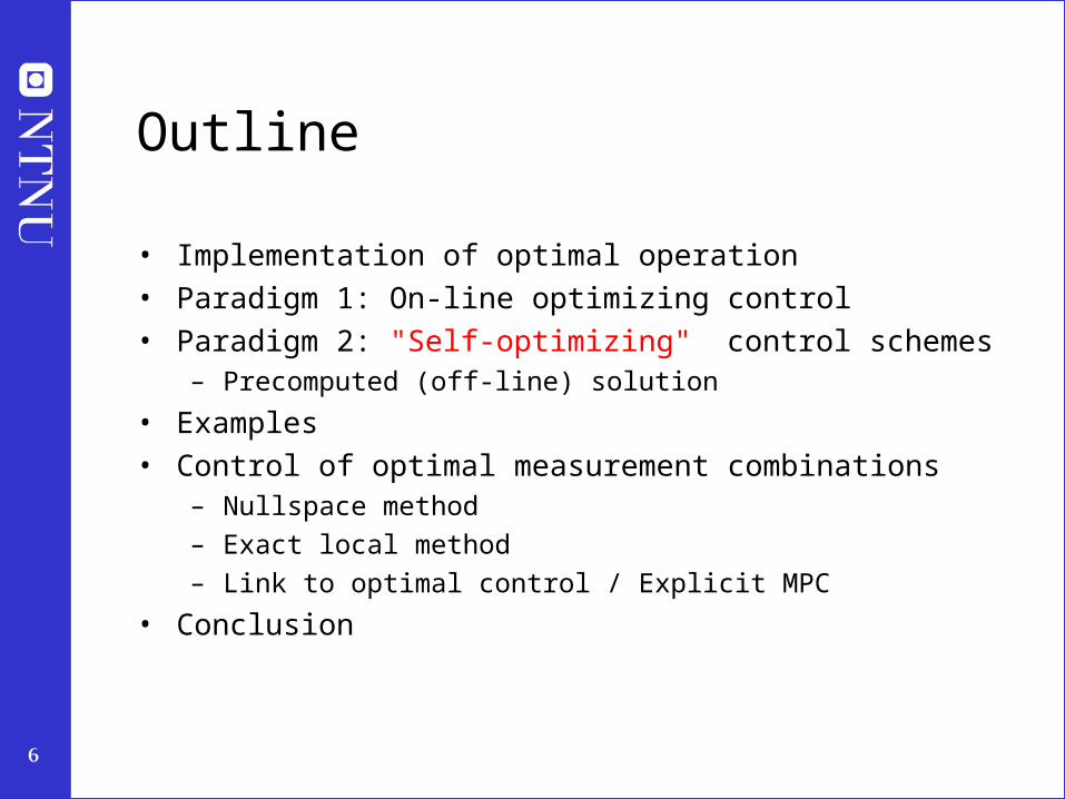
Example paradigm 1: On-line optimizing control of Marathon runner

• Even getting a reasonable model requires > 10 PhD’s … and the model has to be fitted to each individual….

• Clearly impractical!

13

Implementation: Paradigm 2

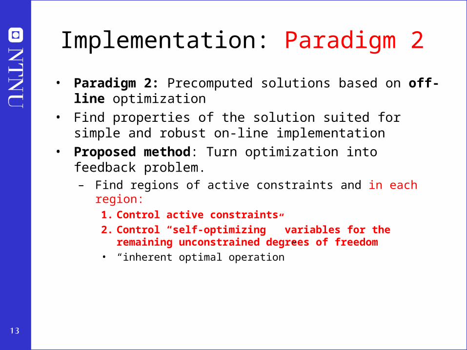
• Paradigm 2: Precomputed solutions based on off-line optimization

• Find properties of the solution suited for simple and robust on-line implementation

• Proposed method: Turn optimization into feedback problem.– Find regions of active constraints and in each region:

1. Control active constraints

2. Control “self-optimizing ” variables for the remaining unconstrained degrees of freedom

• “inherent optimal operation”

14

Solution 2 – Feedback(Self-optimizing control)

– What should we control?

Optimal operation - Runner

15

Self-optimizing control: Sprinter (100m)

• 1. Optimal operation of Sprinter, J=T– Active constraint control:

• Maximum speed (”no thinking required”)

Optimal operation - Runner

16

• Optimal operation of Marathon runner, J=T• Any self-optimizing variable c (to control at

constant setpoint)?• c1 = distance to leader of race

• c2 = speed

• c3 = heart rate

• c4 = level of lactate in muscles

Optimal operation - Runner

Self-optimizing control: Marathon (40 km)

17

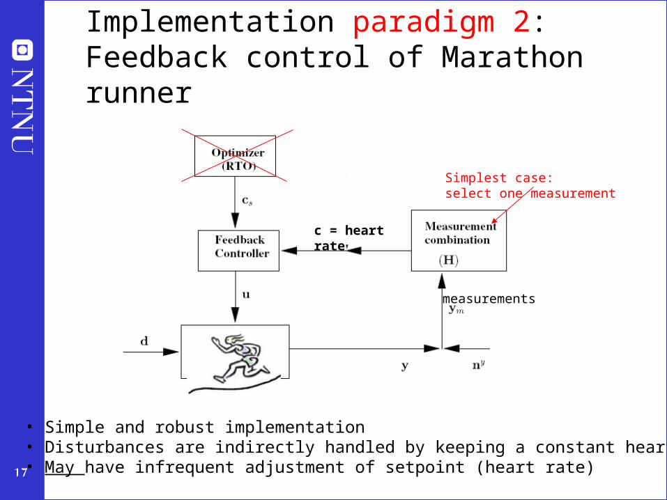
Implementation paradigm 2: Feedback control of Marathon runner

c = heart rate

Simplest case:select one measurement

• Simple and robust implementation• Disturbances are indirectly handled by keeping a constant heart rate• May have infrequent adjustment of setpoint (heart rate)

measurements

18

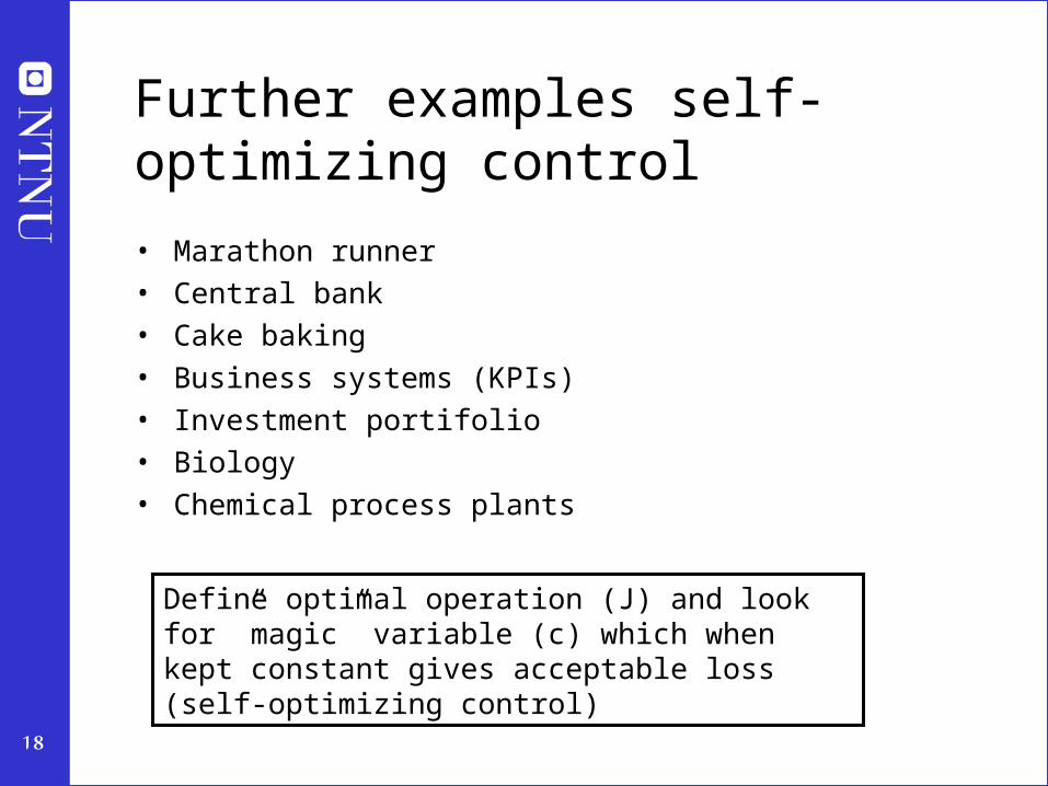
Further examples self-optimizing control

• Marathon runner

• Central bank

• Cake baking

• Business systems (KPIs)

• Investment portifolio

• Biology

• Chemical process plants

Define optimal operation (J) and look for ”magic” variable (c) which when kept constant gives acceptable loss (self-optimizing control)

19

More on further examples

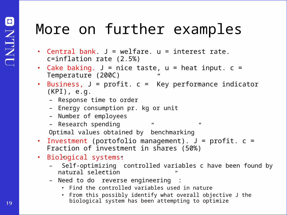
• Central bank. J = welfare. u = interest rate. c=inflation rate (2.5%)• Cake baking. J = nice taste, u = heat input. c = Temperature (200C)• Business, J = profit. c = ”Key performance indicator (KPI), e.g.

– Response time to order– Energy consumption pr. kg or unit– Number of employees– Research spendingOptimal values obtained by ”benchmarking”

• Investment (portofolio management). J = profit. c = Fraction of investment in shares (50%)

• Biological systems:– ”Self-optimizing” controlled variables c have been found by natural

selection– Need to do ”reverse engineering” :

• Find the controlled variables used in nature• From this possibly identify what overall objective J the biological system has

been attempting to optimize

20

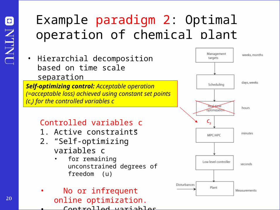
Example paradigm 2: Optimal operation of chemical plant

• Hierarchial decomposition based on time scale separation

Self-optimizing control: Acceptable operation (=acceptable loss) achieved using constant set points (cs) for the controlled variables c

csControlled variables c1. Active constraints2. “Self-optimizing” variables c

• for remaining unconstrained degrees of freedom (u)

• No or infrequent online optimization.

• Controlled variables c are found based on off-line analysis.

21

Summary feedback approach: Turn optimization into setpoint tracking

Issue: What should we control to achieve indirect optimal operation ? Primary controlled variables (CVs):

1. Control active constraints!

2. Unconstrained CVs: Look for “magic” self-optimizing variables!

Need to identify CVs for each region of active constraints

22

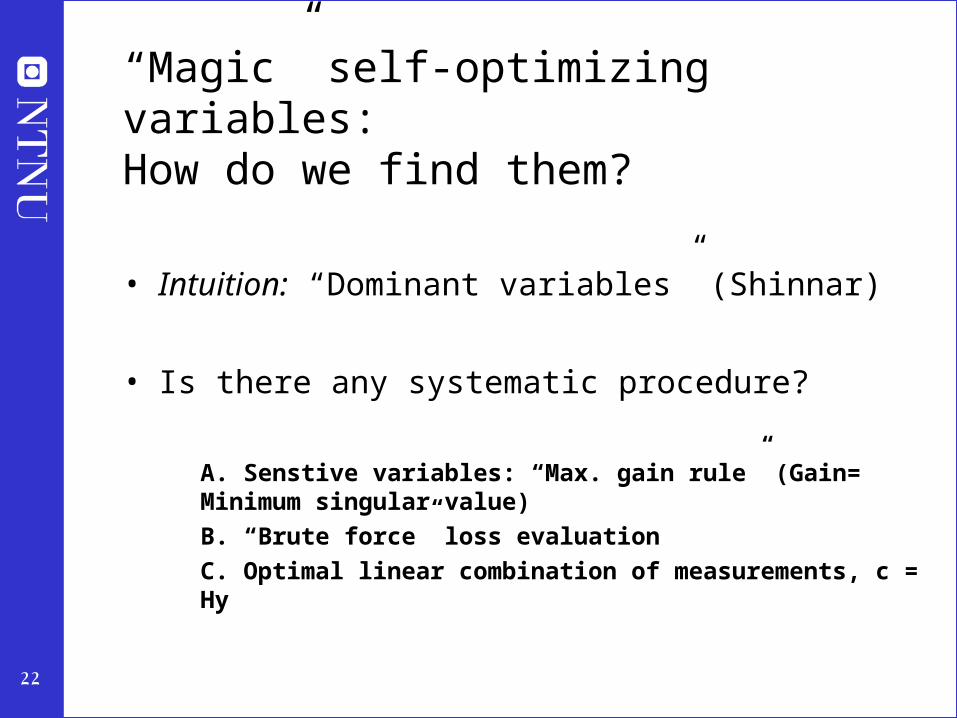
“Magic” self-optimizing variables: How do we find them?

• Intuition: “Dominant variables” (Shinnar)

• Is there any systematic procedure?

A. Senstive variables: “Max. gain rule” (Gain= Minimum singular value)

B. “Brute force” loss evaluation

C. Optimal linear combination of measurements, c = Hy

23

Optimal operation

Cost J

Controlled variable cccoptopt

JJoptopt

Unconstrained optimum

24

Optimal operation

Cost J

Controlled variable cccoptopt

JJoptopt

Two problems:

• 1. Optimum moves because of disturbances d: copt(d)

• 2. Implementation error, c = copt + n

d

n

Unconstrained optimum

25

Candidate controlled variables c for self-optimizing control

Intuitive

1. The optimal value of c should be insensitive to disturbances (avoid problem 1)

2. Optimum should be flat (avoid problem 2 – implementation error).

Equivalently: Value of c should be sensitive to degrees of freedom u. • “Want large gain”, |G|

• Or more generally: Maximize minimum singular value,

Unconstrained optimum

BADGoodGood

26

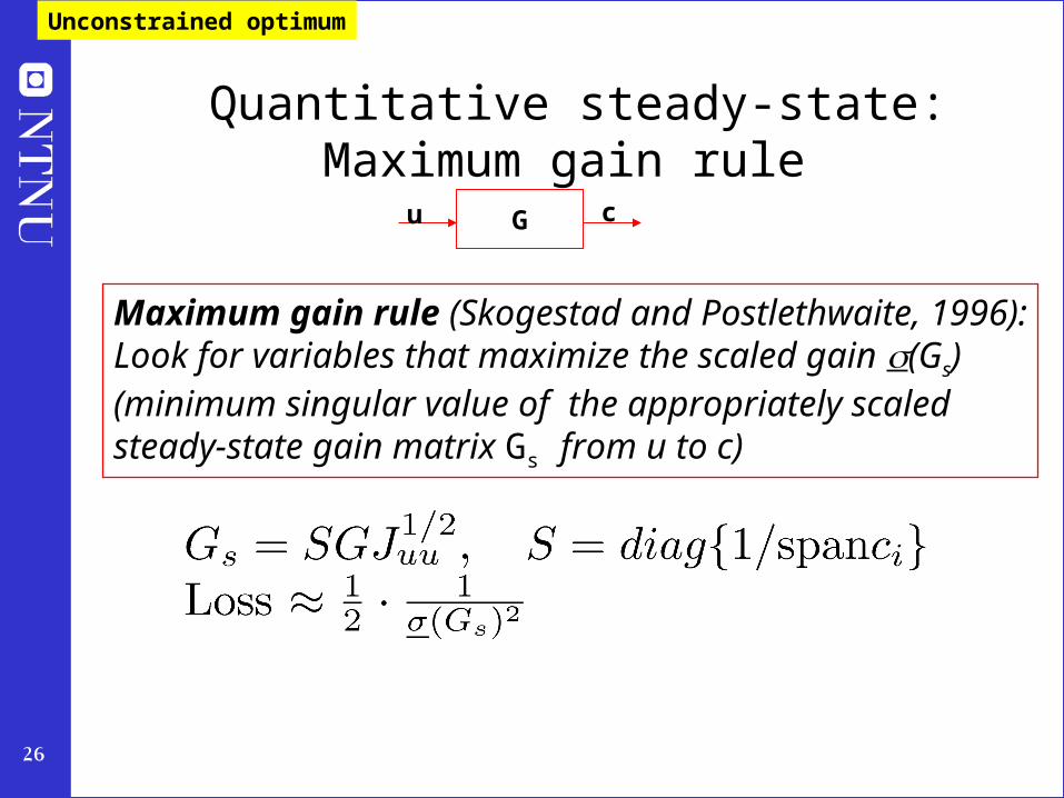
Quantitative steady-state: Maximum gain rule

Maximum gain rule (Skogestad and Postlethwaite, 1996):Look for variables that maximize the scaled gain (Gs) (minimum singular value of the appropriately scaled steady-state gain matrix Gs from u to c)

Unconstrained optimum

Gu c

27

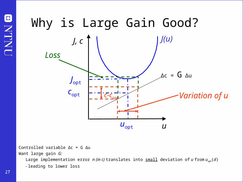
Why is Large Gain Good?

u

J, c

Jopt

uopt

copt c-copt

Loss

Δc = G Δu

Controlled variable Δc = G Δu

Want large gain G:

Large implementation error n (in c) translates into small deviation of u from uopt(d)

- leading to lower loss

Variation of u

J(u)

28

• Operational objective: Minimize cost function J(u,d)

• The ideal “self-optimizing” variable is the gradient (first-order optimality condition (ref: Bonvin and coworkers)):

• Optimal setpoint = 0

• BUT: Gradient can not be measured in practice

• Possible approach: Estimate gradient Ju based on measurements y

• Approach here: Look directly for c without going via gradient

Ideal “Self-optimizing” variables

Unconstrained degrees of freedom:

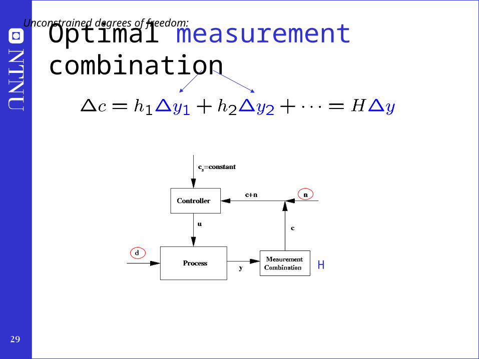
29

Optimal measurement combination

H

Unconstrained degrees of freedom:

30

Amazingly simple!

Sigurd is told by Vidar Alstad how easy it is to find H

Optimal measurement combination

1. Nullspace method for n = 0 (Alstad and Skogestad, 2007)

Basis: Want optimal value of c to be independent of disturbances

• Find optimal solution as a function of d: uopt(d), yopt(d)

• Linearize this relationship: yopt = F d

• Want:

• To achieve this for all values of d:

• Always possible to find H that satisfies HF=0 provided

• Optimal when we disregard implementation error (n)

V. Alstad and S. Skogestad, ``Null Space Method for Selecting Optimal Measurement Combinations as Controlled Variables'', Ind.Eng.Chem.Res, 46 (3), 846-853 (2007).

Unconstrained degrees of freedom:

31

Optimal measurement combination

2. “Exact local method” (Combined disturbances and implementation errors)

• V. Alstad, S. Skogestad and E.S. Hori, ``Optimal measurement combinations as controlled variables'', Journal of Process Control, 19, 138-148 (2009).

Theorem 1. Worst-case loss for given H (Halvorsen et al, 2003):

Unconstrained degrees of freedom:

Applies to any H (selection/combination)

Theorem 2 (Alstad et al. ,2009): Optimization problem to find optimal combination is convex.

32

Example: CO2 refrigeration cycle

Unconstrained DOF (u)Control what? c=?

pH

33

CO2 refrigeration cycle

Step 1. One (remaining) degree of freedom (u=z)

Step 2. Objective function. J = Ws (compressor work)

Step 3. Optimize operation for disturbances (d1=TC, d2=TH, d3=UA)• Optimum always unconstrained

Step 4. Implementation of optimal operation• No good single measurements (all give large losses):

– ph, Th, z, …

• Nullspace method: Need to combine nu+nd=1+3=4 measurements to have zero disturbance loss

• Simpler: Try combining two measurements. Exact local method:

– c = h1 ph + h2 Th = ph + k Th; k = -8.53 bar/K

• Nonlinear evaluation of loss: OK!

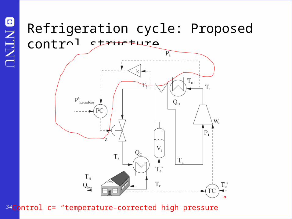
34

Refrigeration cycle: Proposed control structure

Control c= “temperature-corrected high pressure”

35

Summary: Procedure selection controlled variables

1. Define economics (cost J) and operational constraints

2. Identify degrees of freedom and important disturbances

3. Optimize for various disturbances

4. Identify active constraints regions (off-line calculations)

For each active constraint region do step 5-6:

5. Identify “self-optimizing” controlled variables for remaining degrees of freedom

6. Identify switching policies between regions

36

What about optimal control and MPC (model predictive control)?

Paradigm 1: On-line optimizing control where measurements are used to update model and states

Paradigm 2: “Self-optimizing” control scheme found by exploiting properties of the solution

MPC

Optimal control = “Explicit MPC”

37

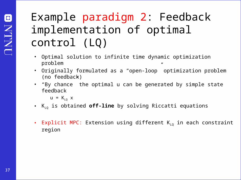
Example paradigm 2: Feedback implementation of optimal control (LQ)

• Optimal solution to infinite time dynamic optimization problem

• Originally formulated as a “open-loop” optimization problem (no feedback)

• “By chance” the optimal u can be generated by simple state feedbacku = KLQ x

• KLQ is obtained off-line by solving Riccatti equations

• Explicit MPC: Extension using different KLQ in each constraint region

38

Example paradigm 2: Explicit MPC

A. Bemporad, M. Morari, V. Dua, E.N. Pistikopoulos, ”The Explicit Linear Quadratic Regulator for Constrained Systems”, Automatica, vol. 38, no. 1, pp. 3-20 (2002).

• Summary: Two paradigms MPC1. Conventional MPC: On-line optimization

2. Explicit MPC: Off-line calculation of KLQ for each region(must determine regions online)

39

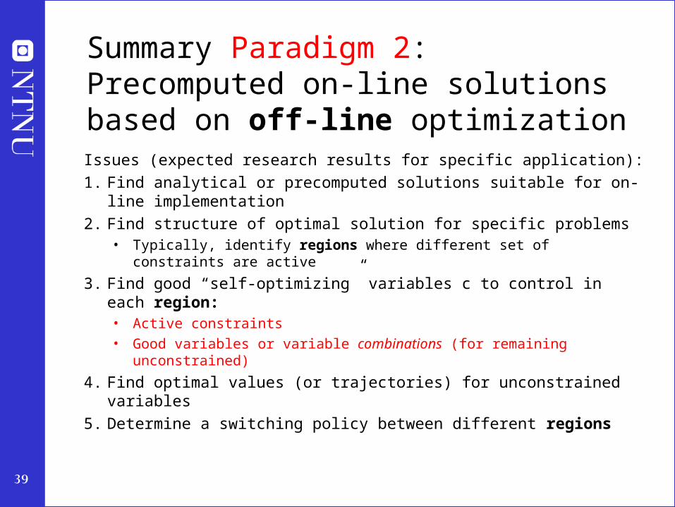
Summary Paradigm 2: Precomputed on-line solutions based on off-line optimizationIssues (expected research results for specific application):

1. Find analytical or precomputed solutions suitable for on-line implementation

2. Find structure of optimal solution for specific problems• Typically, identify regions where different set of constraints are active

3. Find good “self-optimizing” variables c to control in each region:• Active constraints

• Good variables or variable combinations (for remaining unconstrained)

4. Find optimal values (or trajectories) for unconstrained variables

5. Determine a switching policy between different regions

40

Conclusion

• Simple control policies are always preferred in practice (if they exist and can be found)

• Paradigm 2: Use off-line optimization and analysis to find simple near-optimal control policies suitable for on-line implementation

• Current research: Several interesting extensions– Optimal region switching

– Dynamic optimization

– Nonlinear extensions