1

Practical Psychology 1

Week 5

Relative frequency, introduction to probability

2

Example:

We want to order shoes for 12 girls Measure the shoe-sizes of 12 girls in

Greece N = 12 (sizes: 39, 41, 40, 37, etc). If the mean shoe-size turns out to be

39.25, does this mean we should order 12 pairs of size 39.6?

In some situations, calculating the mean (as a measure of averageness) would not be useful.

3

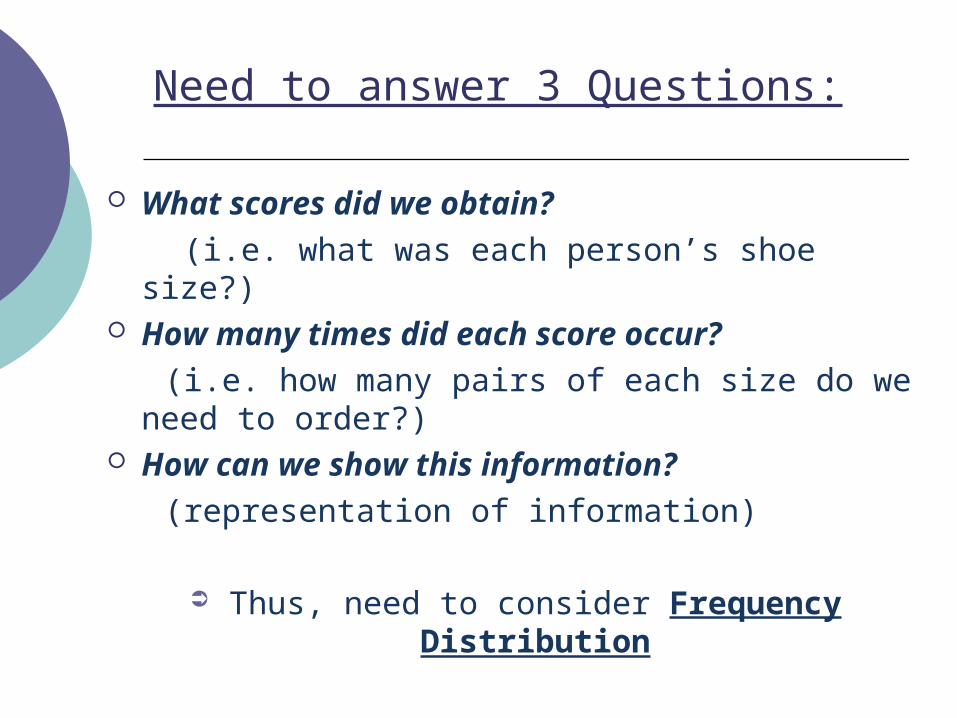
Need to answer 3 Questions:

What scores did we obtain? (i.e. what was each person’s shoe size?) How many times did each score occur? (i.e. how many pairs of each size do we need to

order?) How can we show this information? (representation of information)

Thus, need to consider Frequency Distribution

4

Some definitions…

Frequency (f) – the number of times a score occurs in a set of data

Frequency Distribution or histogram – a graph showing how many times each score occurs.

What scores did we obtain? How many times did each score occur?

5

Constructing Frequency Distributions:

Tables Ungrouped Frequency distributions Grouped Frequency distributions

HistogramsStem-and-leaf plotsBar charts

6

TABLE: Ungrouped Frequency Distribution

• Score = N of relatives

• Freq = N of people with that particular number of relatives

• N = 10

(i.e. entire sample size)

7

Example: IQ

We could measure each person’s IQ score out of 100.

This data could be represented as an ungrouped frequency distribution (like the previous slide)

OR…

8

Grouped Frequency Distribution

• Note that the class intervals are equal

• Class interval = 10

• Need to select intervals carefully (must not be too narrow or too wide).

9

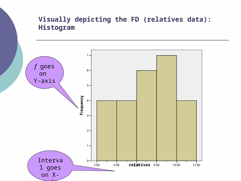
Visually depicting the FD (relatives data): Histogram

f goes on

Y-axis

Interval goes on X-axis

relatives

10

Stem and leaf plot: example data

11

Visually depicting the FD: Stem & Leaf plot

LeafLeaf shows shows the final the final

digits of the digits of the scorescore

StemStem shows shows leading leading digitsdigits

12

Remember!

The previous examples work best with interval (or ratio) data

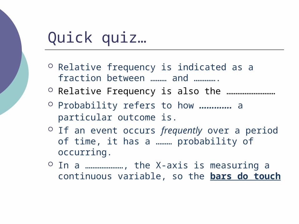
Note that in a histogram, the X-axis is measuring a continuous variable, so the bars do touch.

13

Frequency Distributions with nominal (i.e. categorical) data

• Sample data (N=10): 10 voters interviewed

• n (labour) = 6 • n (con) = 2 • n (lib-dem) = 2• To depict this data,

can draw a bar chart

14

Bar-chart

Bars do NOT touch, as

measuring categorical

variable

15

Relative Frequency and the Normal Curve

Relative frequency is the proportion of the time that a score occurs in a data set.

Indicated as a fraction between 0 and 1

(i.e. 0.1, 0.2, 0.3, 0.4,…1)

16

Relative Frequency

E.g. 1, 2, 2, 2, 3, 4, 4, 5 (N=8)

RF of 2 is 3/8 = 0.375 = 0.38 (note: round off to 2 dp).

Therefore, the score of 2 has a RF of 0.38 in the above data set.

17

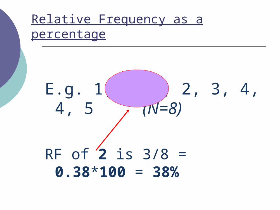
Relative Frequency as a percentage

E.g. 1, 2, 2, 2, 3, 4, 4, 5 (N=8)

RF of 2 is 3/8 = 0.38*100 = 38%

18

RF and the Normal Curve

Area under the curve is 100% of the sample So a proportion of the area under the curve

corresponds to a proportion of the scores (i.e. the relative frequency)

19

Examples

If a score occurs 32% of the time, its relative frequency is 0.32

If a score’s relative frequency is 0.46, it occurs 46% of the time

Scores that occupy 0.2 (20/100) of the area under the curve have a relative frequency of 0.2

20

Cumulative Frequency as a Percentage

10 + 45 = 5510 + 45 = 55 2.5 + 7.5 = 102.5 + 7.5 = 10

21

Suggested Reading

FIELD, A. (2009). Discovering Statistics using

SPSS (3rd ed.). London: Sage. pp. 18-20.

LANGDRIDGE, D. (2004). Introduction to

research methods and data analysis in

Psychology. Harlow: Pearson – Prentice Hall. pp.

123-127.

Introduction to Probability

23

What is probability?

E.g. coin: p (getting Heads) = 1 in 2 or 0.5 or 50% Probability can be expressed as a ratio, fraction, or

percentage.

Probability (p) describes random or chance events

refers to how likely a particular outcome is.

Event must be random (i.e. not rigged), so outcome be determined by luck.

24

Probability of events occurring is measured on a scale from

0 (not possible) to 1 (must happen).

0 1

25

Probability and Relative Frequency

• If an event occurs frequently over a period of

time, high probability of occurring.• If an event occurs infrequently over a period

of time, low probability of occurring.

This judgment is the event’s relative frequency,

which is equal to it’s probability (see next slide

for example)

26

Probability and Relative Frequency

RF of “4” occurring on a throw of a die is 1/6: • 1 = frequency of event, • 6 = total number of possible outcomes• 1/6 = 0.167 (the RF of landing a “4”)

Relative Frequency is also the probability, so: • p (throwing a 4) = 0.167• p (not throwing a 4) = 1 - 0.167 = 0.833 • Both probabilities should add up to 1.

In research (or in life!), probabilities are often somewhere in between 0 and 1 - nothing is absolutely uncertain (or certain).

27

Probability Distributions

A probability distribution indicates the probability of all possible outcomes.

Very simple To create a true

probability distribution, need to observe the entire population.

However, this isn’t always possible, so the probability distribution may be based on observations from a sample.

Score on Die P (getting score on die)

1 0.167

2 0.167

3 0.167

4 0.167

5 0.167

6 0.167

28

Creating a probability distribution from a sample, based on actual observations

The arrival of a bus is observed for 21 days. Days on time = 7 Days late = 14

The Probability distribution on the basis of above sample is:

p (on time) = 7/21 = 0.33 p (late) = 14/21 = 0.67

Quick quiz…

Relative frequency is indicated as a fraction between ……… and ………….

Relative Frequency is also the ………………………

Probability refers to how …………. a particular outcome is.

If an event occurs frequently over a period of time, it has a ……… probability of occurring.

In a …………………, the X-axis is measuring a continuous variable, so the bars do touch

Let’s work on some exercises