1. PREAMBLE - asti.edu.in Manual Control System and Simulation 1 Department of Electrical & Electronics

Laboratory Manual Control System and Simulation

1 Department of Electrical & Electronics Engineering ASTRA

1. PREAMBLE:

Control Systems Lab consists of multiple workstations, each equipped with an oscilloscope,

digital multi-meter, PID trainers, control system trainers and stand alone inverted-pendulum,

ball and beam control, magnetic-levitation trainers. This lab also covers the industrial

implementation of advanced control systems via different computer tools such as MATLAB and

Simulink.



2 OBJECTIVE & RELEVANCE

The aim of this Control system laboratory is to provide sound knowledge in the basic concepts

of linear control theory and design of control system, to understand the methods of

representation of systems and getting their transfer function models, to provide adequate

knowledge in the time response of systems and steady state error analysis, to give basic

knowledge is obtaining the open loop and closed–loop frequency responses of systems and to

understand the concept of stability of control system and methods of stability analysis. It helps

the students to study the compensation design for a control system. This lab consist of DC,AC

servomotor, synchros, DC position control, PID controller kit with temperature control, lead lag

compensator kit, PLC kit, Stepper ,process control simulator

OUTCOME

After the completion of this course student able solve the control system problems by using the programs through MATLAB.

Determination of transfer function useful to design the systems. Introducing of MATLAB in control systems solutions



3 List of Experiments:

1. Time Response of Second order system

2. Study of characteristics of Synchros

3. Effect of feedback on DC servo motor

4. Transfer function of DC motor

5. Effect of P, PD, PI, PID controller on a second order systems

6. Simulation of OP – AMP based integrator and differentiator

7. Study of Lag leg compensation

8. Characteristics of magnetic amplifier

9. Root locus plot, Bode plot from MATLAB

10. State space model for classical transfer function using MATLAB Verification

11. Characteristics of AC servo motor

12. Programmable logic controller



4. Text and Reference Books

TEXT BOOKS :

T1 : B. C. Kuo “Automatic Control Systems” 8th edition– by 2003– John wiley and son’s., T2 : I. J. Nagrath and M. Gopal, “Control Systems Engineering” New Age International (P)

Limited, Publishers, 2nd edition. REFERENCE BOOKS :

R1 : Katsuhiko Ogata “Modern Control Engineering” Prentice Hall of India Pvt. Ltd., 3rd edition, 1998.

R2 : N.K.Sinha, “Control Systems” New Age International (P) Limited Publishers, 3rd

Edition,1998. R3 : NISE “Control Systems Engg.” 5th Edition – John wiley R4 : Narciso F. Macia George J. Thaler, “ Modeling & Control Of Dynamic Systems”

Thomson Publishers



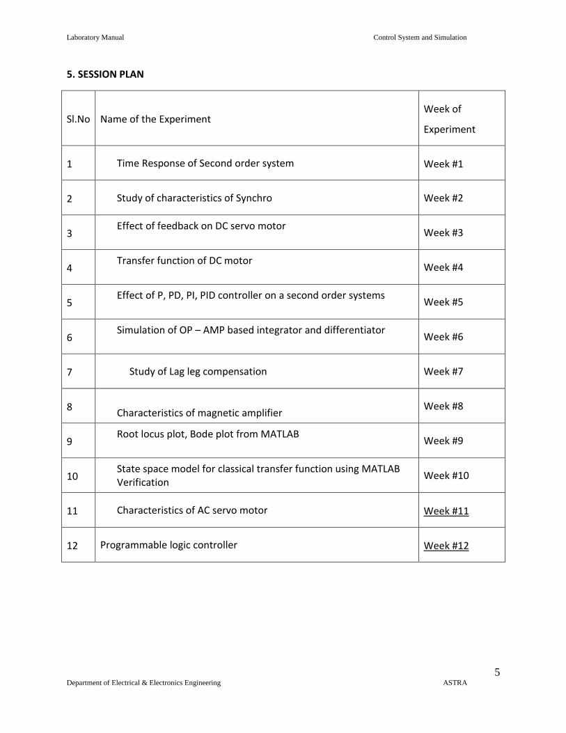
5. SESSION PLAN

Sl.No Name of the Experiment Week of

Experiment

1 Time Response of Second order system Week #1

2 Study of characteristics of Synchro Week #2

3 Effect of feedback on DC servo motor

Week #3

4 Transfer function of DC motor

Week #4

5 Effect of P, PD, PI, PID controller on a second order systems

Week #5

6 Simulation of OP – AMP based integrator and differentiator

Week #6

7 Study of Lag leg compensation Week #7

8 Characteristics of magnetic amplifier

Week #8

9 Root locus plot, Bode plot from MATLAB

Week #9

10 State space model for classical transfer function using MATLAB Verification

Week #10

11 Characteristics of AC servo motor Week #11

12 Programmable logic controller Week #12



6 Experiment write up

6.1. TIME RESPONSE OF SECOND ORDER SYSTEM

AIM :

To obtain the time response of a second order system. APPARATUS :

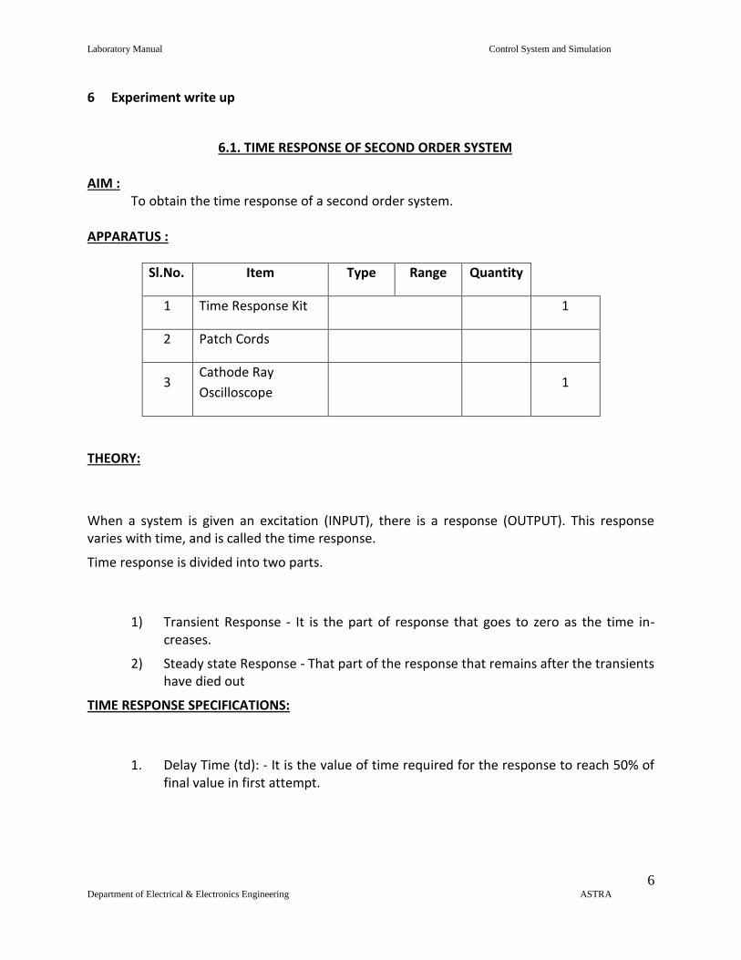
Sl.No. Item Type Range Quantity

1 Time Response Kit 1

2 Patch Cords

3 Cathode Ray

Oscilloscope

1

THEORY:

When a system is given an excitation (INPUT), there is a response (OUTPUT). This response varies with time, and is called the time response.

Time response is divided into two parts.

1) Transient Response - It is the part of response that goes to zero as the time in-creases.

2) Steady state Response - That part of the response that remains after the transients have died out

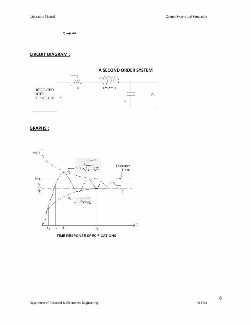
TIME RESPONSE SPECIFICATIONS:

1. Delay Time (td): - It is the value of time required for the response to reach 50% of final value in first attempt.



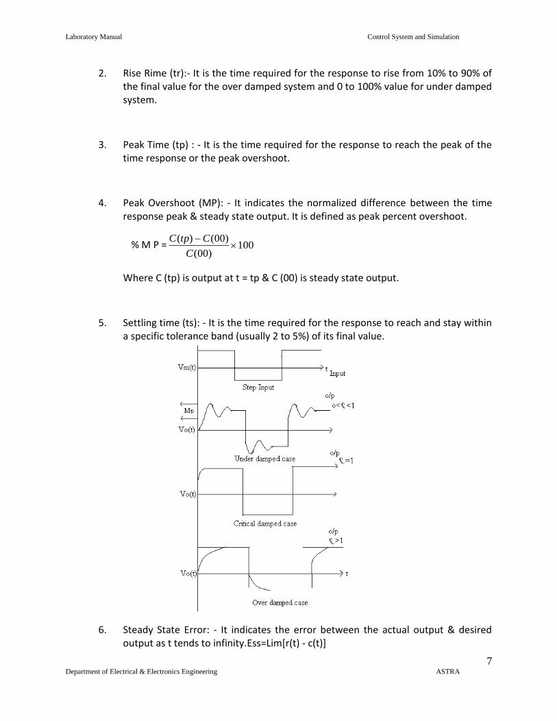
2. Rise Rime (tr):- It is the time required for the response to rise from 10% to 90% of the final value for the over damped system and 0 to 100% value for under damped system.

3. Peak Time (tp) : - It is the time required for the response to reach the peak of the time response or the peak overshoot.

4. Peak Overshoot (MP): - It indicates the normalized difference between the time response peak & steady state output. It is defined as peak percent overshoot.

% M P = 100)00(

)00()(

C

CtpC

Where C (tp) is output at t = tp & C (00) is steady state output.

5. Settling time (ts): - It is the time required for the response to reach and stay within a specific tolerance band (usually 2 to 5%) of its final value.

6. Steady State Error: - It indicates the error between the actual output & desired output as t tends to infinity.Ess=Lim[r(t) - c(t)]



t ∞

CIRCUIT DIAGRAM :

A SECOND ORDER SYSTEM

GRAPHS :



PROCEDURE :

1. Make connections as shown in circuit diagram.

2. Connect repeated step input to RLC circuit.

3. Make power on to the unit.

4. Connect C.R.O. at the output and adjust C.R.O. to get stable pattern on C.R.O.

5. Vary R by potentiometer and for a given set of values of L & C, note down R for

critically damped response

6. Vary R to obtain under damped response and measure R value, time response

specifications.

7. Plot the same response on Graph paper.

NOTE: Actual value of R is R + resistance of Inductance

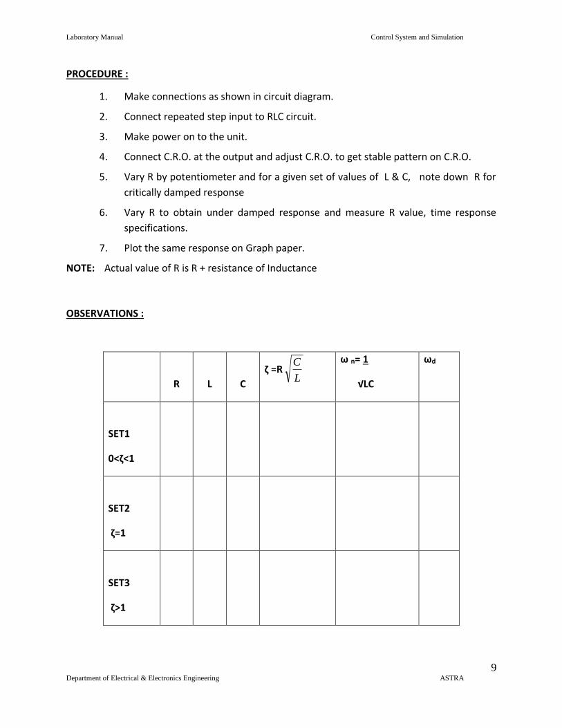
OBSERVATIONS :

R

L

C

ζ =RL

C

ω n= 1

√LC

ωd

SET1

0<ζ<1

SET2

ζ=1

SET3

ζ>1



PRECAUTIONS :

1. Loose connections are to be avoided.

2. Circuit connections should not be made while power is on.

3. Readings of meters must be taken without parallax error.

RESULT: Time Response specifications are obtained

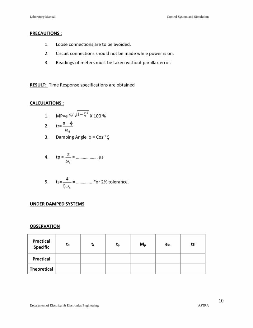
CALCULATIONS :

1. MP=e-/21 X 100 %

2. tr=d

3. Damping Angle = Cos-1

4. tp = d

= ………………. s

5. ts=n

4

= ………….. For 2% tolerance.

UNDER DAMPED SYSTEMS

OBSERVATION

Practical Specific

td tr tp Mp ess ts

Practical

Theoretical



6.2 STUDY OF CHARACTERISTICS OF SYNCHROS

AIM :

To study the characteristics of synchro transmitter and receiver system.

APPARATUS :

S.NO ITEM TYPE RANGE QUANTITY

1 Synchros Kit 1

2 Patch Cords

3 Multimeter 1

THEORY :

The term synchro is a generic name for a family of inductive devices which works on the

principle of a rotating transformer basically they are electro- mechanical devices or

electromagnetic transducers which produces an o/p voltage depending upon angular position

of the rotor a synchro system is formed by inter connection. The basic synchro is usually called

a synchro transmitter. Its construction is similar to that of a three phase alternator. The stator

(stationary member) is of laminated silicon steel and is slotted to accommodate a balanced

three phase winding which is usually of concentric coil type f (three identical coils are placed in

the stator with their axis 120 degree apart) and is Y connected. The rotor is a dumb bell shape

type in construction and wound with a concentric coil. An a.c. voltage is applied to the rotor

winding through slip rings. The system set up is consists of synchro transmitter and synchro

receiver on a single rigid panel housed in MS cabinet plates, Rotor position of Tx and Rx is

marked by graduated angular scale with pointer arrangement. AC input excitation supply for



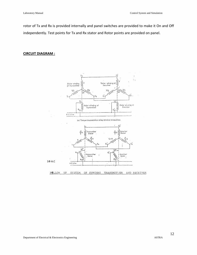
rotor of Tx and Rx is provided internally and panel switches are provided to make it On and Off

independently. Test points for Tx and Rx stator and Rotor points are provided on panel.

CIRCUIT DIAGRAM :

1Ф A.C

Supply



PROCEDURE :

1. Connect the mains supply to the unit.

2. Varying rotor position of Transmitter in steps of 300 note down VS1S2, VS2S3, VS3S1

readings.

3. Connect S1, S2, S3 of Transmitter to S1, S2, S3 of receiver respectively.

4. Move the rotor of synchro Transmitter in steps of 30 degrees and note down the

change in Receiver rotor.

5. Enter the input angular position Transmitter rotor and output angular position of

Receiver rotor in tabular form and plot a graph.

6. Plot graph settings :

a) (Vs1s2, Vs2s3, Vs3s1) Vs θt

b) θr Vs θt



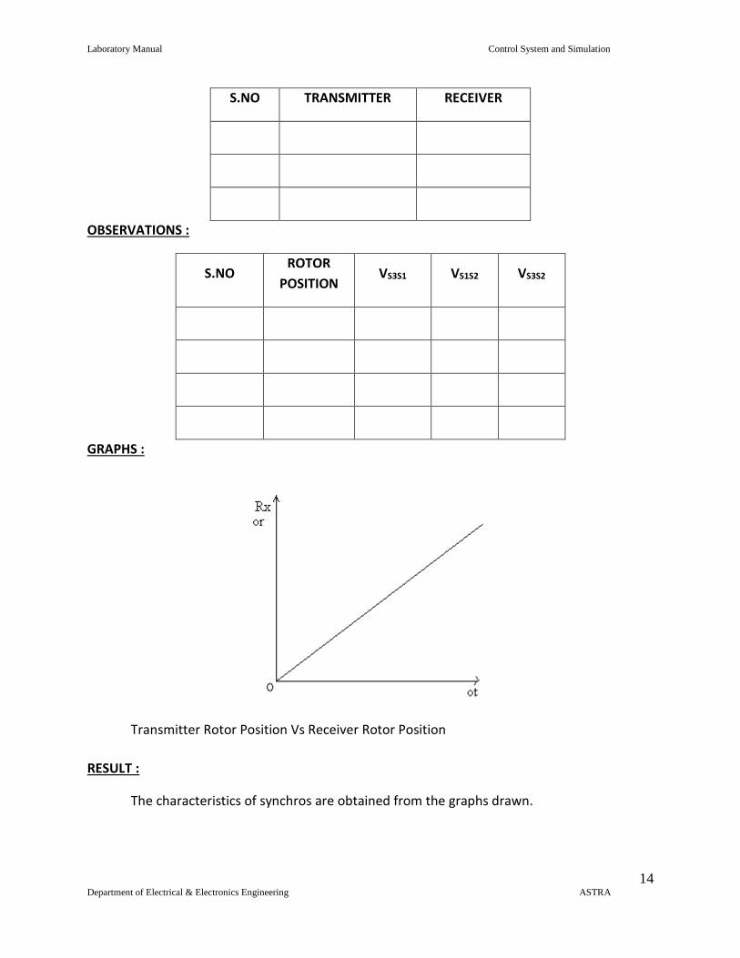
S.NO TRANSMITTER RECEIVER

OBSERVATIONS :

S.NO ROTOR

POSITION VS3S1 VS1S2 VS3S2

GRAPHS :

Transmitter Rotor Position Vs Receiver Rotor Position

RESULT :

The characteristics of synchros are obtained from the graphs drawn.



6.3. EFFECT OF FEED BACK ON DC SERVO MOTOR

AIM :

To Study the effect feed back on D C Servomotor.

APPARATUS :

S.No ITEM Type Range Quantity

1 D.C servomotor kit 1

2 Patch cords As required

PROCEDURE :

1. Switch on the main power supply to the kit without the connecting the feedback path.

2. Adjust it to Zero position by using Zero adjustment knob.

3. Varying the input potentiometer (P1) & Tabulate the angular displacement (P5) of Servo motor

4. Note the observation in tabular form

5. Switch off the power supply now connect the feed back path.

6. Switch on the power supply and adjust the gain knob to certain value.



7. Varying the input potentiometer (P1) & Tabulate the angular displacement (P5) of Servo motor.

8. Repeat the procedure for 2 or 3 values of gain. Plot the graph between input and output angular displacement potent

9. Now tabulated the comments observed before and after feed back.

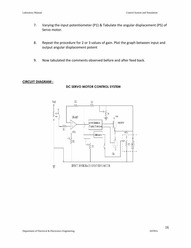
CIRCUIT DIAGRAM :

DC SERVO MOTOR CONTROL SYSTEM



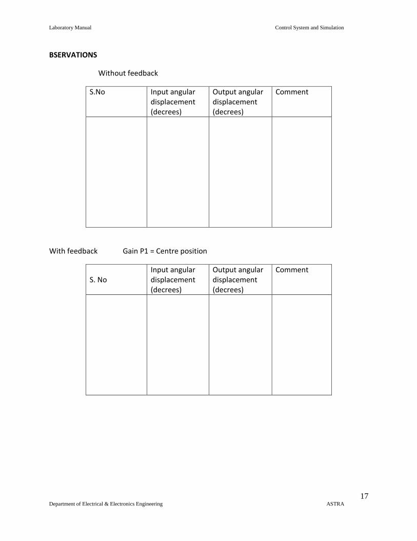
BSERVATIONS

Without feedback

S.No Input angular displacement (decrees)

Output angular displacement (decrees)

Comment

With feedback Gain P1 = Centre position

S. No

Input angular displacement (decrees)

Output angular displacement (decrees)

Comment



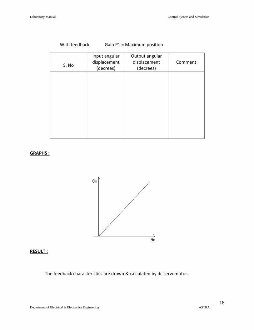
With feedback Gain P1 = Maximum position

S. No

Input angular displacement

(decrees)

Output angular displacement

(decrees) Comment

GRAPHS :

RESULT :

The feedback characteristics are drawn & calculated by dc servomotor.



6.4. CHARACTERISTICS OF DC SERVO MOTOR

AIM :

To Study the D C Servomotor characteristics.

APPARATUS :

S.No ITEM Type Range Quantity

1 D.C servomotor kit 1

2 Multimeter 2

3 Patch cords

THEORY :

DC Servomotor are broadly classified as:-

i) Armature controlled dc servomotor.

ii) Field controlled dc servomotor.

In Armature controlled DC Servo motor the field is excited by a constant dc supply.

If the field current is constant then speed is directly proportional to armature voltage and

torque is proportional to armature current. Hence torque and speed can be controlled by

armature voltage reversible operation is possible by reversing the armature voltage. In

small motors the armature voltage is controlled by a variable resistance.



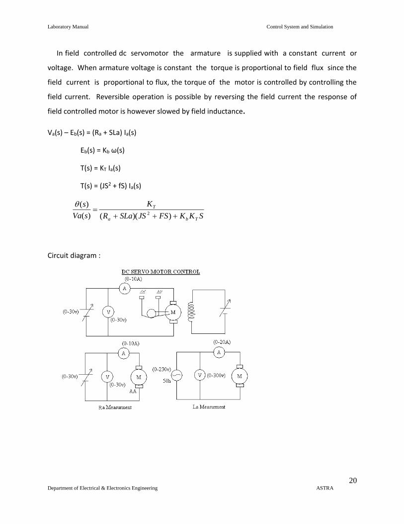
In field controlled dc servomotor the armature is supplied with a constant current or

voltage. When armature voltage is constant the torque is proportional to field flux since the

field current is proportional to flux, the torque of the motor is controlled by controlling the

field current. Reversible operation is possible by reversing the field current the response of

field controlled motor is however slowed by field inductance.

Va(s) – Eb(s) = (Ra + SLa) Ia(s)

Eb(s) = Kb ω(s)

T(s) = KT Ia(s)

T(s) = (JS2 + fS) Ia(s)

SKKFSJSSLaR

K

sVa

s

Tba

T

))(()(

)(2

Circuit diagram :



PROCEDURE :

A) CONNECTION

1. Connect the power supply cables of motor to respective A, AA, F FF terminals on the kit.

2. Connect the speed measurement chord to the kit

B) DETERMINATION OF KT

1. Switch on the power supply to the kit.

2. Vary the armature voltage such that the motor runs at rated speed

3. Take the no load readings of Va, Ia, Vf, If, speed and S1, S2

4. Repeat the step 3 by loading the machine, for 5 to 6 different sets of loads for 10v.

5. Calculate torque T= (S2 – S1) 9.81 r.

6. Plot the graph between torque TVs Ia, to obtain KT

C) DETERMINATION OF Kb

1. Conect the circuit as per the circuit diagram and switch on the main power supply

2. Varying the armature voltage in steps and note down Va, Ia , Speed.

3. Bring the armature voltage pot to minimum porition and switch off the supply.

4. Calculate back emf Eb = Va – Ia Ra

5. Plot graph between Eb Vs N and determine the slope of the curve, to obtain Kb

D) DETERMINATION OF Ra

1. Conect the circuit as per the circuit diagram

2. Ensuring that armature is connected to D.C. supply. Switch on the main power

supply.

3. Vary the armature voltage in steps and note down armature current

4. Determine Ra = Va/Ia and take the average of it



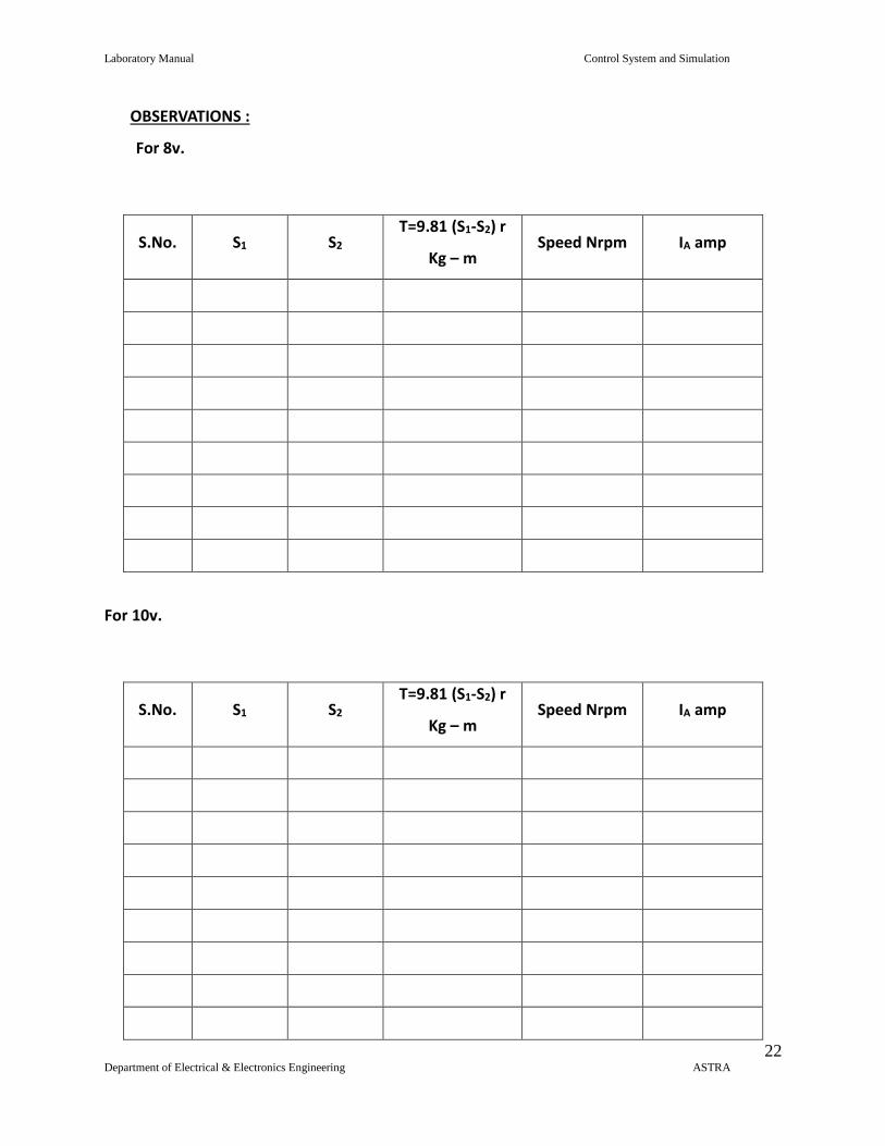
OBSERVATIONS :

For 8v.

S.No. S1 S2 T=9.81 (S1-S2) r

Kg – m Speed Nrpm IA amp

For 10v.

S.No. S1 S2 T=9.81 (S1-S2) r

Kg – m Speed Nrpm IA amp



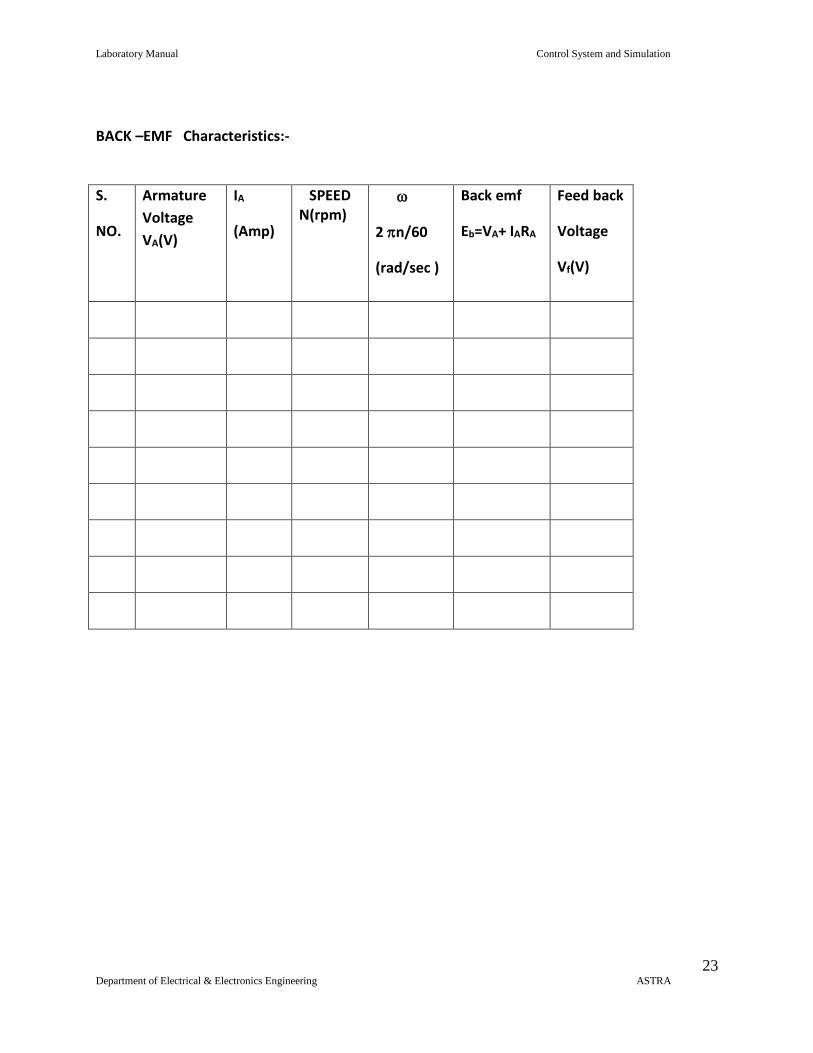
BACK –EMF Characteristics:-

S.

NO.

Armature

Voltage

VA(V)

IA

(Amp)

SPEED N(rpm)

2 n/60

(rad/sec )

Back emf

Eb=VA+ IARA

Feed back

Voltage

Vf(V)



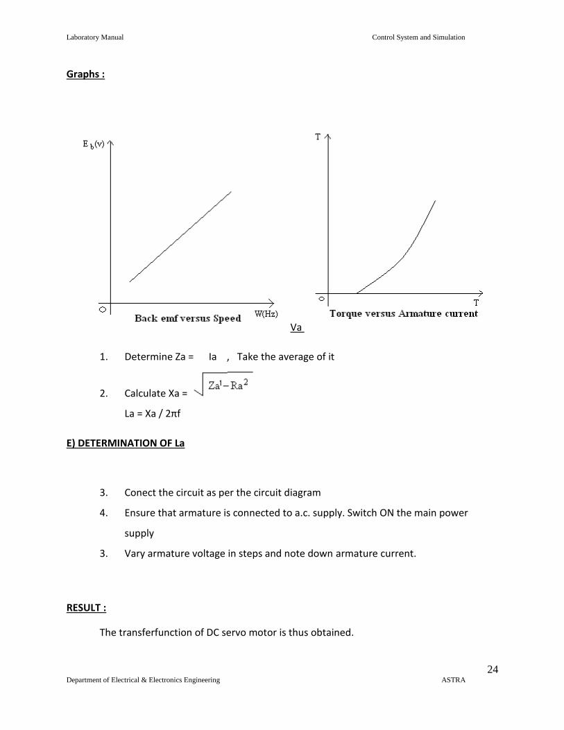
Graphs :

Va

1. Determine Za = Ia , Take the average of it

2. Calculate Xa =

La = Xa / 2πf

E) DETERMINATION OF La

3. Conect the circuit as per the circuit diagram

4. Ensure that armature is connected to a.c. supply. Switch ON the main power

supply

3. Vary armature voltage in steps and note down armature current.

RESULT :

The transferfunction of DC servo motor is thus obtained.



6.5 EFFECT OF P, PD, PI, PID CONTROLLER ON A SECOND ORDER SYSTEM

AIM :

To observe the effect of P,PD,PI,PID Controller on Second Order System.

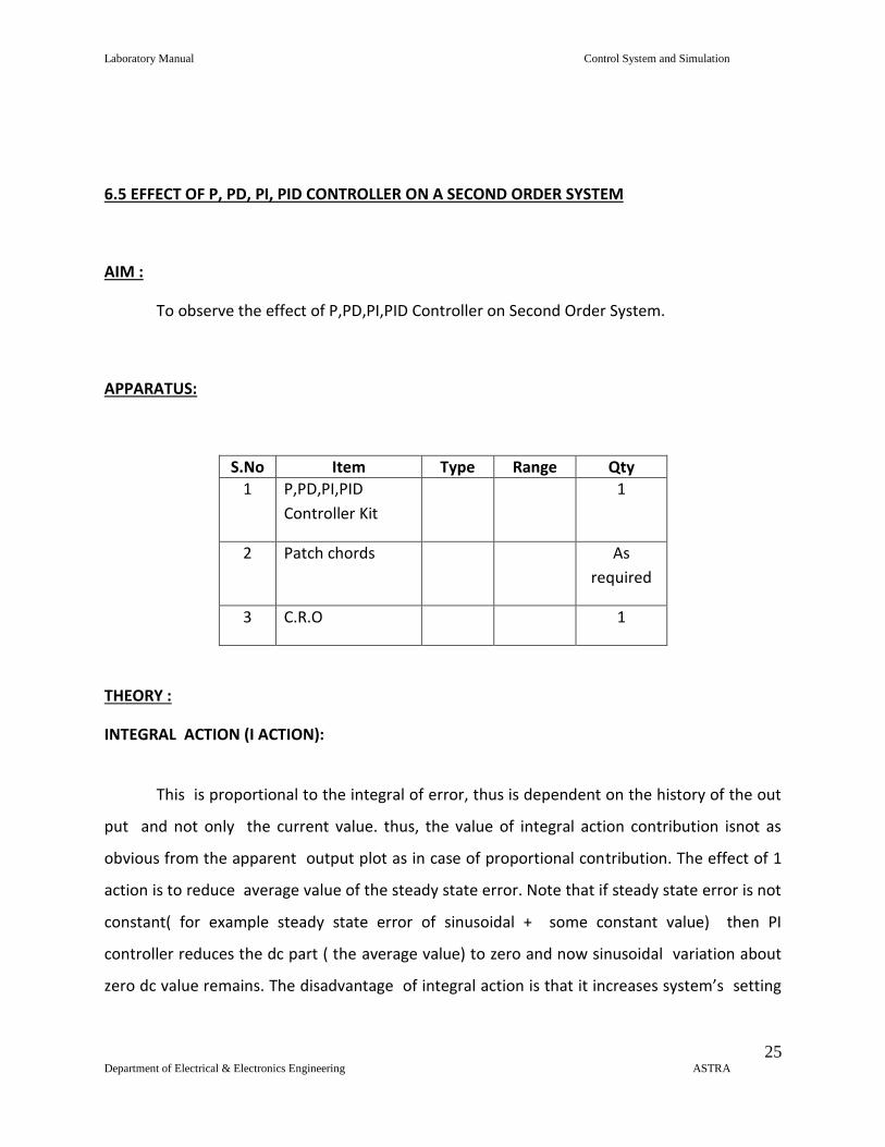
APPARATUS:

S.No Item Type Range Qty

1 P,PD,PI,PID

Controller Kit

1

2 Patch chords As

required

3 C.R.O 1

THEORY :

INTEGRAL ACTION (I ACTION):

This is proportional to the integral of error, thus is dependent on the history of the out

put and not only the current value. thus, the value of integral action contribution isnot as

obvious from the apparent output plot as in case of proportional contribution. The effect of 1

action is to reduce average value of the steady state error. Note that if steady state error is not

constant( for example steady state error of sinusoidal + some constant value) then PI

controller reduces the dc part ( the average value) to zero and now sinusoidal variation about

zero dc value remains. The disadvantage of integral action is that it increases system’s setting



time. A typical output plot with PI action (proportional+ integral) is shown below. For this Kd is

set to zero.

DERIVATIVE ACTION (D ACTION):

The third term of PID controller transfer equation contributes proportional to the time

derivative of error (or rate of change of error). This part is introduced to compensate against

the output variations with respect to time.

If steady state error is not constant (for example steady state error of sinusoidal+ some

constant value) then PD controller reduces the varying part to zero and the constant steady

error of average value remains.

The D action depends on few past and the current error value and not the complete

history as in case of integral action. The contribution is high - speed changes in output that

may occur because of various reasons. This

also responds to the output variations that may rise due to noise in the sensing, conditioning

and feedback network which is unnecessary and hence these parts must be precision type.

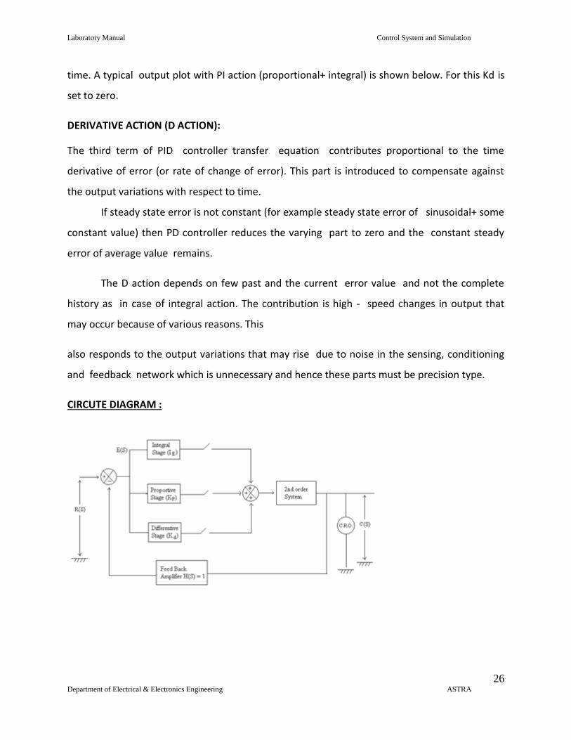
CIRCUTE DIAGRAM :



PROCEDURE :

1. Connect the circuit as per the block diagram shown

2. Switch ON the main power supply and select Input square wave signal of certain amplitude and frequency. Note the input waveform from C.R.o.

P-Controller:

3. Switch ON Proportional stage keeping integral, derivative stage in OFF position

4. Vary the proportional gain KP for 3 to 4 values and note down the Output C(S) waveforms for each value.

PD Controller:

5. Switch ON derivative stage keeping integeral stage OFF and fix KP at certain value.

6. Vary Derivative gain Dt for 3 to 4 values and Note down the Output C(S) waveforms for each value

PI Controller:

7. Switch OFF Dt stage, Switch ON Integral stage and Fix KP at certain value

8. Vary Integral gain Int for 3 to 4 values and note down the output C(S) waveforms for each value.

PID Controller:

9. Switch ON all the three controllers fix derivative, Integral controller at certain values.

10. Vary proportional controller gain KP and note down output C(S) waveforms.

11. Compare the output waveforms for different controller gains and write remarks on the effects of various controller gains on 2nd order system time response specifications.

RESULT :

The effect of P, PI, PD, PID controllers are studied



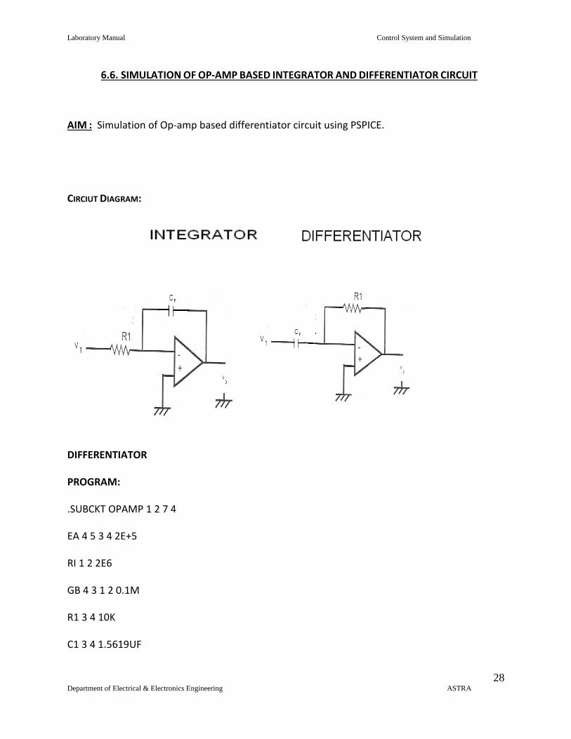
6.6. SIMULATION OF OP-AMP BASED INTEGRATOR AND DIFFERENTIATOR CIRCUIT

AIM : Simulation of Op-amp based differentiator circuit using PSPICE.

CIRCIUT DIAGRAM:

DIFFERENTIATOR

PROGRAM:

.SUBCKT OPAMP 1 2 7 4

EA 4 5 3 4 2E+5

RI 1 2 2E6

GB 4 3 1 2 0.1M

R1 3 4 10K

C1 3 4 1.5619UF



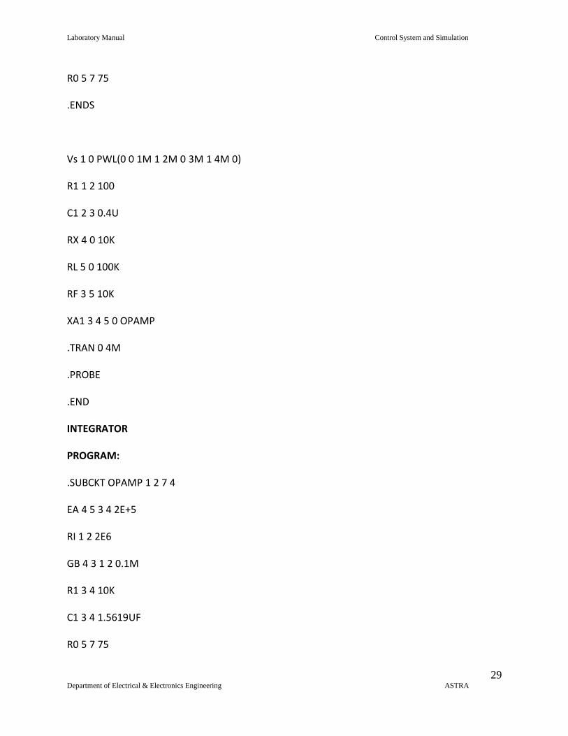
R0 5 7 75

.ENDS

Vs 1 0 PWL(0 0 1M 1 2M 0 3M 1 4M 0)

R1 1 2 100

C1 2 3 0.4U

RX 4 0 10K

RL 5 0 100K

RF 3 5 10K

XA1 3 4 5 0 OPAMP

.TRAN 0 4M

.PROBE

.END

INTEGRATOR

PROGRAM:

.SUBCKT OPAMP 1 2 7 4

EA 4 5 3 4 2E+5

RI 1 2 2E6

GB 4 3 1 2 0.1M

R1 3 4 10K

C1 3 4 1.5619UF

R0 5 7 75



.ENDS

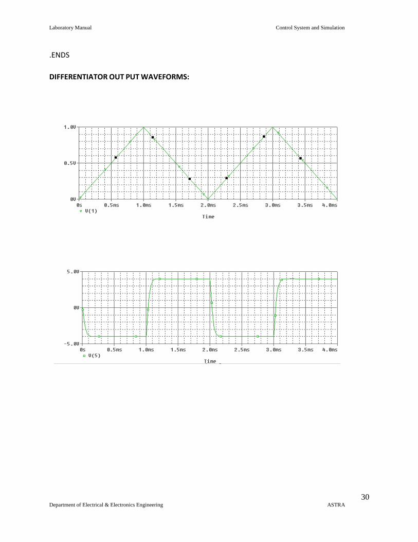
DIFFERENTIATOR OUT PUT WAVEFORMS:



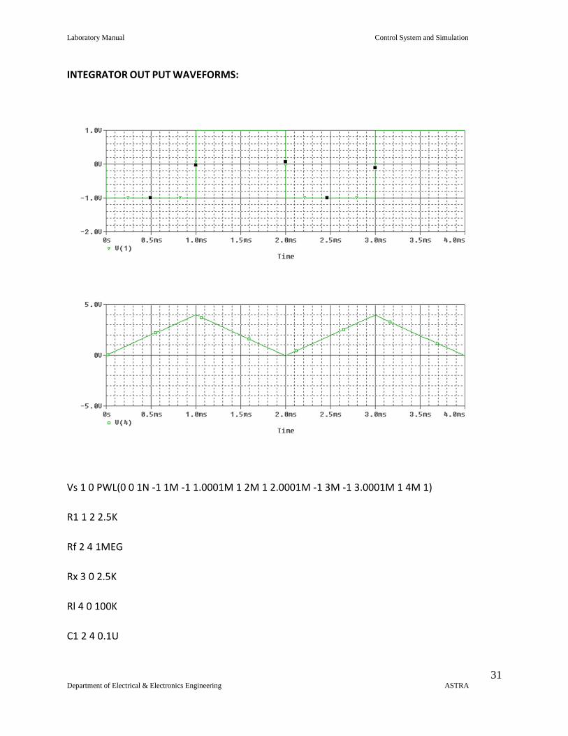
INTEGRATOR OUT PUT WAVEFORMS:

Vs 1 0 PWL(0 0 1N -1 1M -1 1.0001M 1 2M 1 2.0001M -1 3M -1 3.0001M 1 4M 1)

R1 1 2 2.5K

Rf 2 4 1MEG

Rx 3 0 2.5K

Rl 4 0 100K

C1 2 4 0.1U



XA1 2 3 4 0 OPAMP

.TRAN 0 4M

.PROBE

.END

Procedure :

1. Represent nodes for the given circuit

2. Write PSPICE program in the PSPICE text editor and run the program

3. Make the connections if required

4. Observe the output and plot the waveform

RESULT:



6.7 STUDY OF LAG LEAD COMPENSATION

AIM :

To study the characteristics of lag lead compensators

APPARATUS :

S.No Item Type Range Quantity

1.

LAG LEAD Trainee kit

1

2

Patch cords

3 Multimeter 2

Theory :

Passive electric components –resistors, capacitors and inductors are used for

implementation of a compensator. However the inductor is a very bulky component at low

frequencies, passive networks are made up of only resistors and capacitors are used in practice.

Condition for reliability of transfer function D(s) with passive resistor capacitor (RC) networks is

that all finite poles of D(s) may lie anywhere in s-plane. By taking an operational amplifier to the

output of passive RC network, it is possible to realize a specified gain of the compensator.

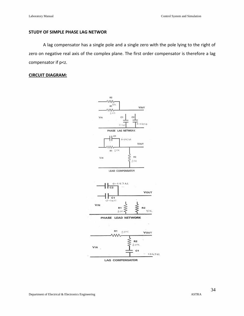
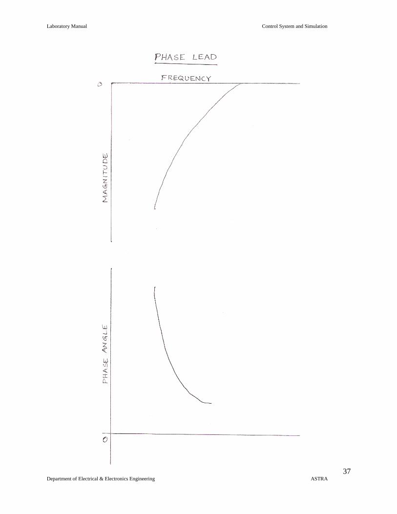
STUDY OF SIMPLE PHASE LEAD NETWORK:

Lead compensator has a single pole and a single zero with the pole lying to the left of the zero

on the negative real axis of the complex plane. The first order compensator is a lead

compensator if p>z.



STUDY OF SIMPLE PHASE LAG NETWOR

A lag compensator has a single pole and a single zero with the pole lying to the right of

zero on negative real axis of the complex plane. The first order compensator is therefore a lag

compensator if p<z.

CIRCUIT DIAGRAM:



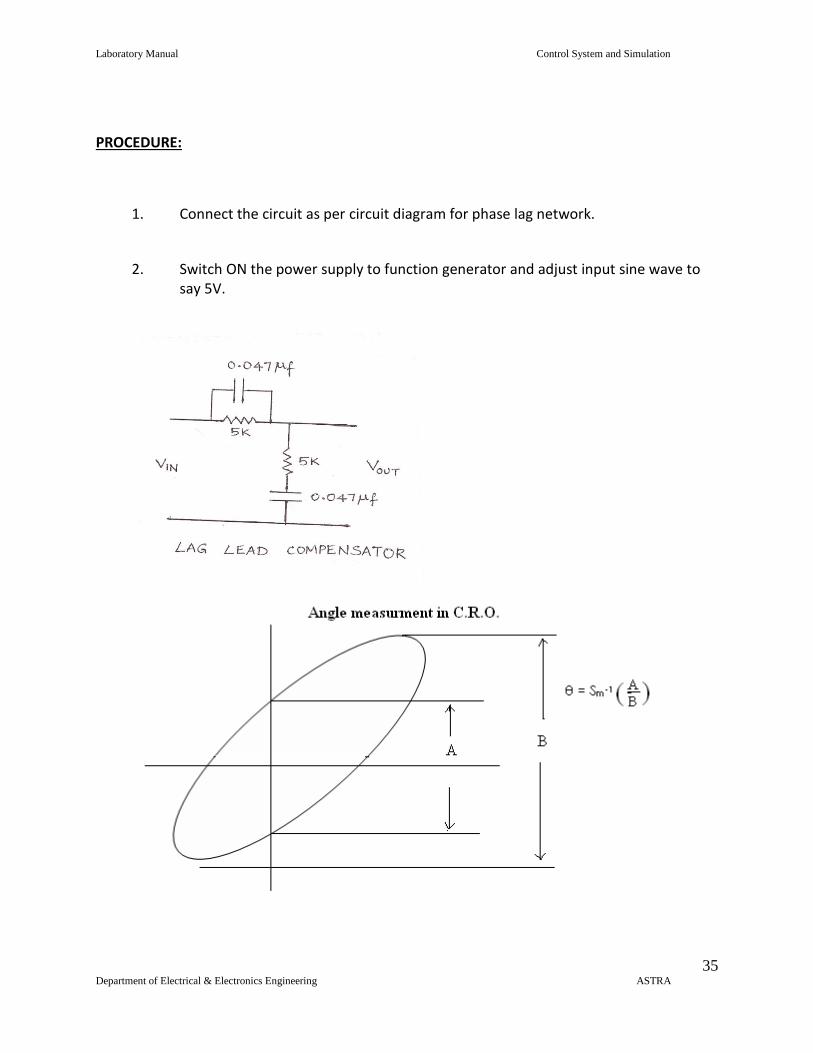
PROCEDURE:

1. Connect the circuit as per circuit diagram for phase lag network.

2. Switch ON the power supply to function generator and adjust input sine wave to say 5V.



3. C.R.O. is to be connected in X-Y made for phase displacement measurement connect X-input of CRO to input of lag network and Y- input of C.R.O to output of lag network.

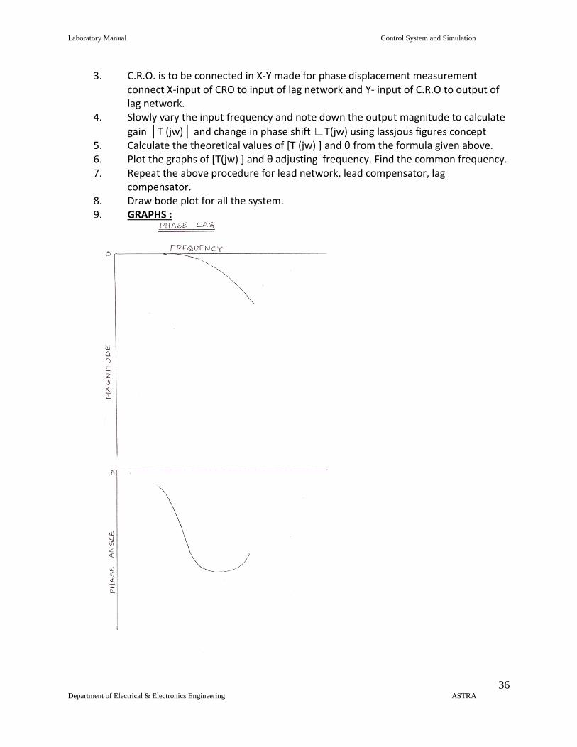
4. Slowly vary the input frequency and note down the output magnitude to calculate

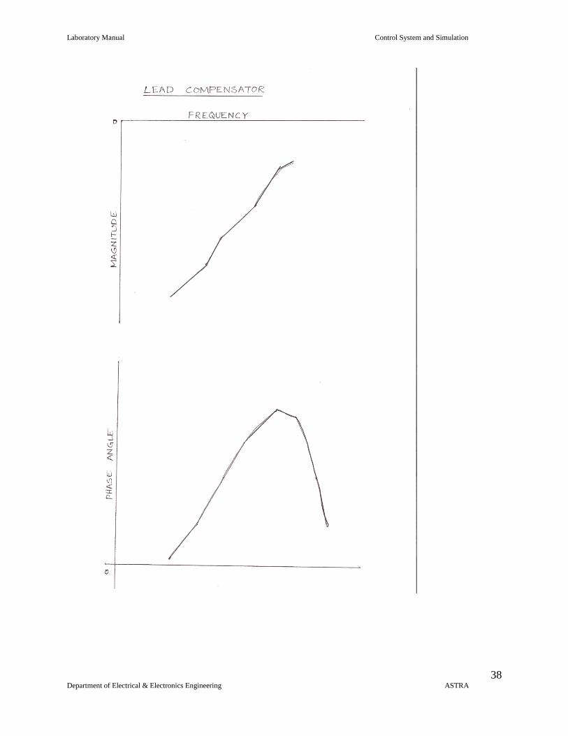
gain │T (jw)│ and change in phase shift ∟T(jw) using lassjous figures concept 5. Calculate the theoretical values of [T (jw) ] and θ from the formula given above. 6. Plot the graphs of [T(jw) ] and θ adjusting frequency. Find the common frequency. 7. Repeat the above procedure for lead network, lead compensator, lag

compensator. 8. Draw bode plot for all the system. 9. GRAPHS :









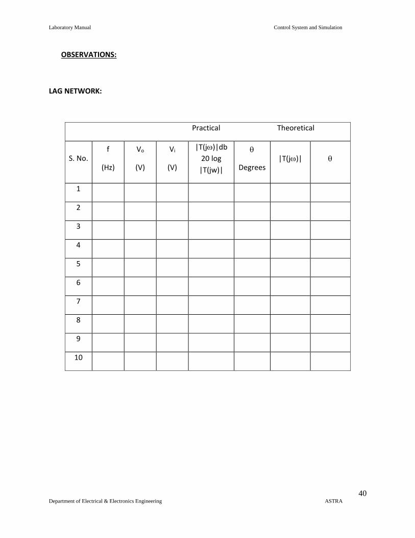
OBSERVATIONS:

LAG NETWORK:

Practical Theoretical

S. No. f

(Hz)

Vo

(V)

Vi

(V)

|T(j)|db

20 log

|T(jw)|

Degrees |T(j)|

1

2

3

4

5

6

7

8

9

10



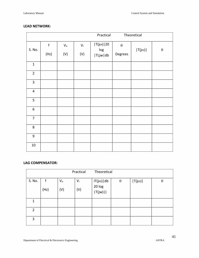
LEAD NETWORK:


S. No. f

(Hz)

Vo

(V)

Vi

(V)

|T(j)|20

log

|TLjw|db

Degrees |T(j)|

1

2

3

4

5

6

7

8

9

10

LAG COMPENSATOR:


S. No. f

(Hz)

Vo

(V)

Vi

(V)

IT(j)|db

20 log

|T(jw)|)

|T(j)|

1

2

3



4

5

6

7

8

9

10

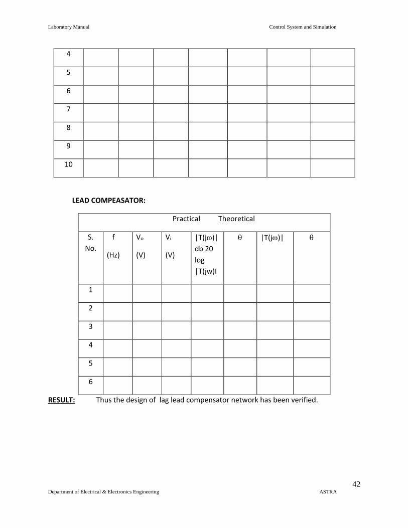
LEAD COMPEASATOR:


S.

No.

f

(Hz)

Vo

(V)

Vi

(V)

|T(j)|

db 20

log

|T(jw)I

|T(j)|

1

2

3

4

5

6

RESULT: Thus the design of lag lead compensator network has been verified.



6.8. CHARACTERISTICS OF MAGNETIC AMPLIFIER

AIM:

To study the characteristics of magnetic amplifier.

S.NO ITEM TYPE RANGE QUANTITY

1 Magnetic Amplifier Kit

1

2 Patch Cords

3 Multimeter 1

APPARATUS:

THEORY:Amplification is the control of a larger output quantity by the variation of a small

input quantity. Magnetic device used to perform such ctrl is the magnetic amplifier. The

combination of saturable reactor with rectifier is called magnetic amplifier.

Saturable reactor:- This device acts as a variable inductance connected in series with a load

across an a c power supply. It is nothing but a transformer, having two or more windings

around a core of steel core A&B has it’s own ac windings connected her in phase opposition

so that when flux moves to the right with in the upper A coil an equal flux moves to the

left with in the lower B coil with in the ctrl coil Two flux movements are in opposite direction.

There by no objectionable ac voltage is induced in the control winding.

Operation:- Gate winding is when operated sin. O&M the voltage across load is very small. But

if ac supply is increase to the extent core get saturated at MN or OP on magnetization curve,

the inductance of gate winding is reduced & voltage appears across load by passing small dc

through control windings .a definite steady MMF is applied to cause flux in the core to increase

in single direction making it more saturated and increase the o/p voltage across the load.

Magnetic Amplifier :- When Si diode are added in series with each gate winding of the saturable reactor. It becomes self saturated reactor also called as magnetic amplifier.

Effect of connecting diode:- When AC power is first applied to the circuit small magnetizing

current flown in gate winding and produces initial flux x. during first part of second wave the

core flux raises from x to y and during reverse current , the part of y say y flux remains in core.

In succeeding cycles, the flux in core is increase to such an extent that the core operate on the

flat portion of the curve through out the entire half cycle. Thus although no direct current yet

flows in the ctrl



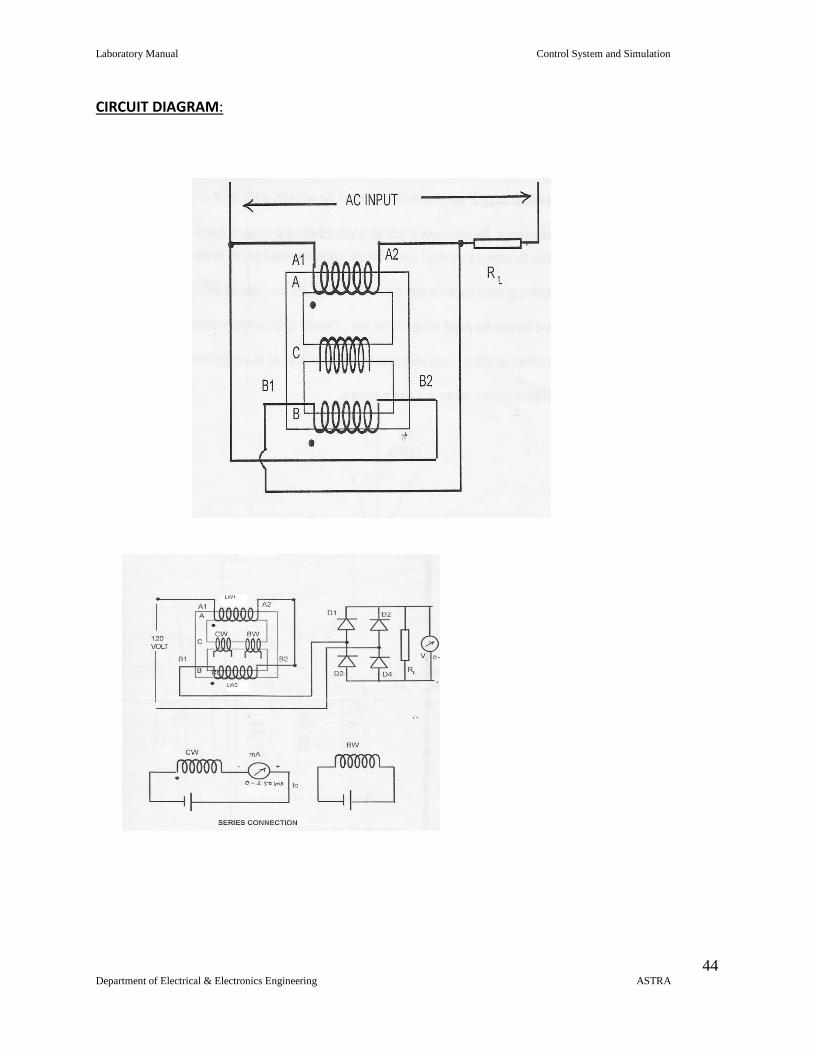
CIRCUIT DIAGRAM:



PROCEDURE:

a) Parallel connection:-

1. Make the connections as shown in circuit diagram.

2. Make power on to the circuit .

3. Keep Cw dc supply and Bw dc supply to zero .note load voltage.

4. Adjust Bw dc supply to get minimum load voltage(VL).

5. Now slowly increase the Cw dc supply in steps and note the ctrl current and load

current .

6. Plot the graph of load current against control current .

7. Calculate the gain of amplifier A=c

L

I

I

.

8. Calculate power gain =DCCD

LL

IV

RV /2

Observations:

Series Connection:-

S.NO IC (ma) VDC(v) VL(v) IL=VL

RL

A= P=



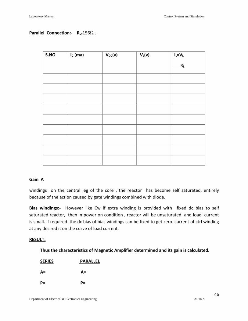
Parallel Connection:- RL=156 .

S.NO IC (ma) VDC(v) VL(v) IL=VL

RL

Gain A

windings on the central leg of the core , the reactor has become self saturated, entirely

because of the action caused by gate windings combined with diode.

Bias windings:- However like Cw if extra winding is provided with fixed dc bias to self

saturated reactor, then in power on condition , reactor will be unsaturated and load current

is small. If required the dc bias of bias windings can be fixed to get zero current of ctrl winding

at any desired it on the curve of load current.

RESULT:

Thus the characteristics of Magnetic Amplifier determined and its gain is calculated.

SERIES PARALLEL

A= A=

P= P=



6.9. ROOT LOCUS AND BODE PLOT USING MAT LAB

AIM: To plot root locus and bode plot from the mat lab.

APPARATUS: Computer with MATLAB software.

THEORY:

COMMAND 1: CLC: It clears the MATLAB command window

COMMAND 2: CLEAR: it clears the MATLAB work shop variables.

COMMAND 3: DISP: Syntax – disp (variable): It displays the variable specified on command

window.

COMMAND 4: PAUSE: With this command the execution will be stopped and it waits for

the enter key.

COMMAND 5: INPUT: Syntax: Variable = Input (‘Comment’);

COMMAND 6: PERCENTAGE: It is used at the beginning of any statement to make it as a

comment in the program.

COMMAND 7: R-LOCUS: Syntax: r locus (Variable): With this we can plot the root locus of any transfer function. That means in the above syntax the variable is nothing but a transfer function.

COMMAND 8: BODE: Syntax: Bode (Variable): With this command we can get bode plot of

the given transfer function.

COMMAND 9: MARGIN: Syntax: Margin (Variable): With this command we can get gain and phase margin of a bode plot of the given transfer function.

COMMAND10: SS: Syntax: Variable1= SS(Variable2): With this command we can get state

space model for the given transfer function. Variable 2 is a transfer function

and variable 1 holds the SS model.

COMMAND11: SS DATA: Syntax: [a,b,c,d] = Ssdata (Variable):

With this command we can retrieve the a,b,c,d matrices of a state space model. Variable holds the state space model.



PROCEDURE:

1. Write the programmme in MATLAB text editor using mat lab instructions for state model of classical transfer function and for transfer function from state model.

2. Run the programs.

3. Note down the outputs.

PROGRAM:

Num = input (“Enter numerator polynomial values in the form of matrix array” );

num = input (“Enter denominator 1 values” );

den = input (“Enter denominator 2 values” );

den = conv (num,den);

H = tf (num,den);

r locus (H);

pause;

Bode(H);

Pause;

Margin(H);

nyquist (H);

pause;

end

RESULT:

The root locus, bode plot and nyquist plot of a transfer function were plotted using

MATLAB software.



6.10. STATE MODEL FOR CLASSICAL TRANSFER FUNCTION & VICE VERSA USING MATLAB

AIM:

To find state model for classical transfer function and transfer function from state

model using MATLAB.

APPARATUS: Computer with MATLAB software

THEORY:

COMMAND 1: CLC: It clears the MATLAB command window

COMMAND 2: CLEAR: it clears the MATLAB work shop variables.

COMMAND 3: DISP: Syntax – disp (variable): It displays the variable specified on command

window.

COMMAND 4: PAUSE: With this command the execution will be stopped and it waits for

the enter key.

COMMAND 5: INPUT: Syntax: Variable = Input (‘Comment’);

COMMAND 6: PERCENTAGE: It is used at the beginning of any statement to make it as a

comment in the program.

COMMAND 7: R-LOCUS: Syntax: r locus (Variable): With this we can plot the root locus of any transfer function. That means in the above syntax the variable is nothing but a transfer function.

COMMAND 8: BODE: Syntax: Bode (Variable): With this command we can get bode plot of

the given transfer function.

COMMAND 9: MARGIN: Syntax: Margin (Variable): With this command we can get gain

and phase margin of a bode plot of the given transfer function.

COMMAND10: SS: Syntax: Variable1= SS(Variable2): With this command we can get state

space model for the given transfer function. Variable 2 is a transfer function

and variable 1 holds the SS model.

COMMAND11: SS DATA:Syntax: [a,b,c,d]=SSdata (Variable):

With this command we can retrieve the a,b,c,d matrices of a state space model. Variable holds the state space model.



PROCEDURE:

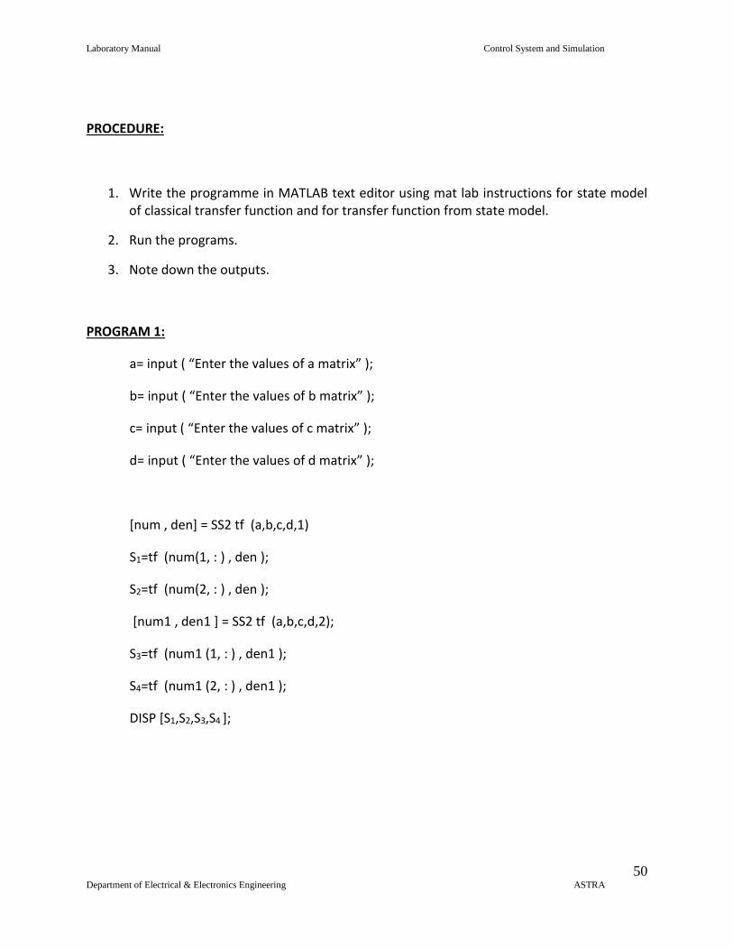
1. Write the programme in MATLAB text editor using mat lab instructions for state model of classical transfer function and for transfer function from state model.

2. Run the programs.

3. Note down the outputs.

PROGRAM 1:

a= input ( “Enter the values of a matrix” );

b= input ( “Enter the values of b matrix” );

c= input ( “Enter the values of c matrix” );

d= input ( “Enter the values of d matrix” );

[num , den] = SS2 tf (a,b,c,d,1)

S1=tf (num(1, : ) , den );

S2=tf (num(2, : ) , den );

[num1 , den1 ] = SS2 tf (a,b,c,d,2);

S3=tf (num1 (1, : ) , den1 );

S4=tf (num1 (2, : ) , den1 );

DISP [S1,S2,S3,S4 ];



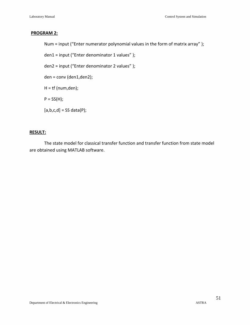
PROGRAM 2:

Num = input (“Enter numerator polynomial values in the form of matrix array” );

den1 = input (“Enter denominator 1 values” );

den2 = input (“Enter denominator 2 values” );

den = conv (den1,den2);

H = tf (num,den);

P = SS(H);

[a,b,c,d] = SS data(P);

RESULT:

The state model for classical transfer function and transfer function from state model

are obtained using MATLAB software.



6.11. CHARACTERISTICS OF AC SERVOMOTOR

AIM:

To determine the speed torque characteristics of AC Servomotor

APPARATUS:

Sl. No. Item Type Range Quantity

1 A.C Servomotor Kit 1

2 Multimeter 1

3 Patch cords

THEORY:

An A.C servomotor is basically a two phase induction motor except for certain special

design features. A two phase induction motor consisting of two stator windings oriented 90

degrees electrically apart in space and excited by a.c voltages which differ in time phase by 90

degrees. Generally voltages of equal magnitude and 90 degrees phase difference are applied to

the two stator phases thus making their respective fields 90 degrees apart in both time and

space at synchronous speed.

The stator windings are excited by voltages of equal r.m.s magnitude & 900 phase

difference these currents give rise to a rotating magnetic field of constant magnitude the

direction of rotation depends of on the phase relationship of the two currents (or voltages)

the exciting currents produce a clock wise rotating magnetic field & phase shift of 1800 in i1

will produce an anti clock wise rotating magnetic field.



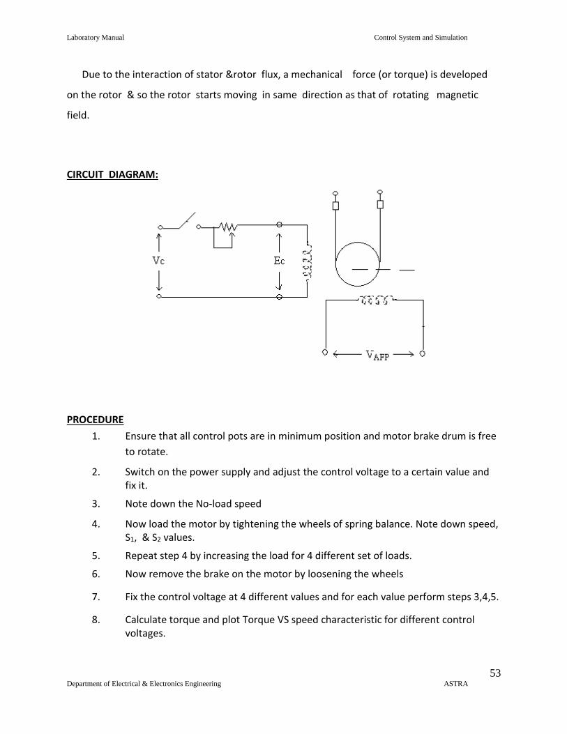
Due to the interaction of stator &rotor flux, a mechanical force (or torque) is developed

on the rotor & so the rotor starts moving in same direction as that of rotating magnetic

field.

CIRCUIT DIAGRAM:

PROCEDURE

1. Ensure that all control pots are in minimum position and motor brake drum is free

to rotate.

2. Switch on the power supply and adjust the control voltage to a certain value and fix it.

3. Note down the No-load speed

4. Now load the motor by tightening the wheels of spring balance. Note down speed, S1, & S2 values.

5. Repeat step 4 by increasing the load for 4 different set of loads.

6. Now remove the brake on the motor by loosening the wheels

7. Fix the control voltage at 4 different values and for each value perform steps 3,4,5.

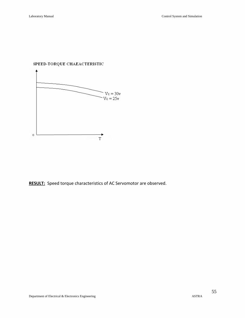
8. Calculate torque and plot Torque VS speed characteristic for different control voltages.



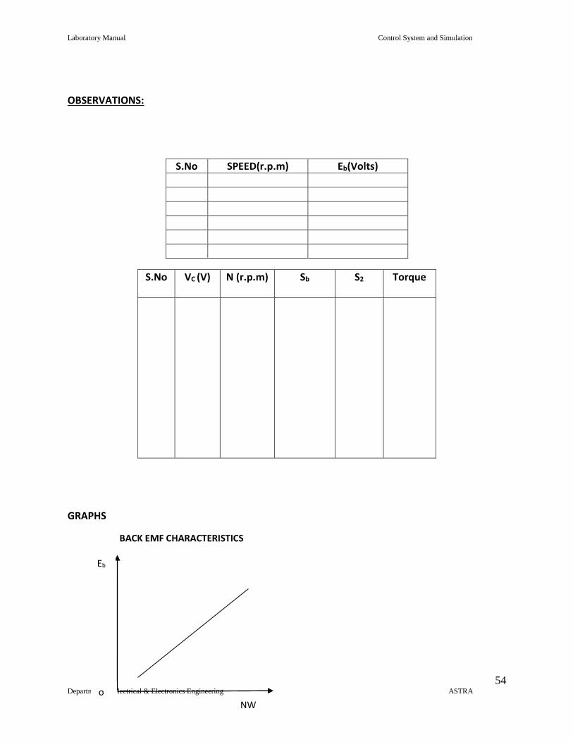
OBSERVATIONS:

S.No VC (V) N (r.p.m) Sb S2 Torque

GRAPHS

S.No SPEED(r.p.m) Eb(Volts)

BACK EMF CHARACTERISTICS

Eb

o NW

(r.p.m)



RESULT: Speed torque characteristics of AC Servomotor are observed.



6.12. PROGRAMMABLE LOGICAL CONTROLLER

AIM:

To implement various logics using PLC trainer

APPARATUS:

PLC – 51 EPROM Chip FANMOTOR COMPUTER CONNECTING CHORD

THEORY:

A programmable controller, formerly called as programmable logic controller PLC can be defined as a solid state device member of the computer family. It is capable of strong instructions to implement control function such as servicing timing, counting arithmetic, data manipulation & communication to control industrial machines & processed. PLC Programming: Implement the following ladder network (shown in figure)

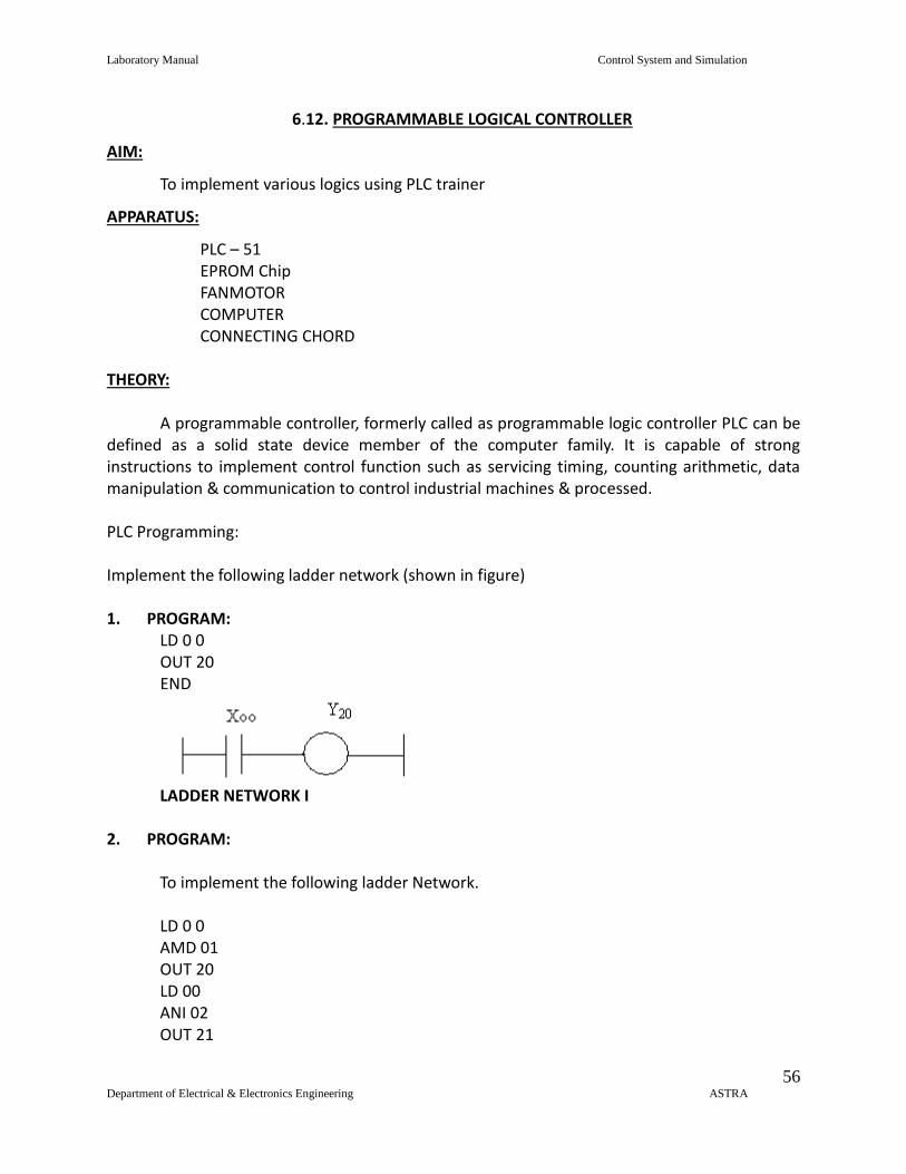
1. PROGRAM:

LD 0 0 OUT 20 END

LADDER NETWORK I

2. PROGRAM:

To implement the following ladder Network. LD 0 0 AMD 01 OUT 20 LD 00 ANI 02 OUT 21



END

LADDER NETWORK II

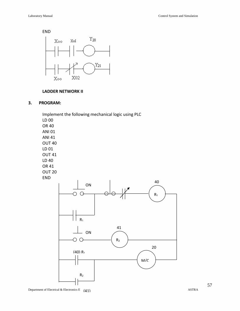
3. PROGRAM: Implement the following mechanical logic using PLC LD 00 OR 40 ANI 01 ANI 41 OUT 40 LD 01 OUT 41 LD 40 OR 41 OUT 20 END

(41)

R1

R2

M/C

(40) R1

41 ON

20

40 ON

R1

R2



MECHANICAL LOGIC USING PLC LOGIC:

The above circuit uses internal relays. There are 16 relays M & M & M. Here we use the

relays 40 & 41. Once 00 is ON & output 20 is ON permanently. Once 01 is ON, R gets off but N is On. So 20 continues to be ON but when 01 is removed 20 gets OFF because M does not have a feedback as mechanism as M.

RESULT:

The above programs



7 Content beyond syllabus:

1) Simulation of block diagram

2) Simulation of practical circuit diagram control system.



8 Sample Viva Voce Questions

Exp 1:

1. What is delay time?

2. What is rise time?

3. What is peak time?

4. What is peak overshoot?

5. What is settling time?

Exp 2:

1. What is a synchro?

2. What is the use of synchro?

3. What is the constructional difference between synchro transmitter & synchro

receiver?

4. What is the relation between a synchro & a transformer?

5. Where do we get maximum e m f in a synchro?

6. When we will get maximum e m f in a synchro?

7. What is the phase different between three voltages induced in the stator of

synchro and why ?

8. How do you determine zero position of synchro

9. what is the error voltage induced ?

Exp 3:

1. What is a servomotor?

2. What are the applications of servomotor?

3. How do you load the D.C Servomotor?

4. Why a servomotor should not be switched on load?

5. What are the elements used as feedback



6. What are the general input and o/p parameters of D.C. servomotor

7. What is the element used as error detector in the given circuit.

Exp 4:

What is a servomotor?


3. How can we get the feed back characteristics of D.C Servomotor?

4. How do you load the D.C Servomotor?


6. What is a mathematical model ? What is its importance?

7. How do you define transfer function? What is its significance?

8. What are Kb, KT

Exp 5:

1. What is the use of a controller in control system?

2. What is the use of proportionality controller?

3. Why is integral controller used?

4. Why is differential controller used?

5. How can you rectify an error using controller?

6. What is meant by sampling network?

7. How do you sense the errors in a control system?

8. What do you mean by tuning of controller?

9. Which controller is most commonly used?

Exp 6:

1. What is the instruction used for plotting bode plot

2. do we get transfer function of a control system using MATLAB?



3. How do you load the A.C Servomotor?

Exp 7:

1. What is the formula for calculating phase angle? 2. What is the formula magnitude of phase lead circuit lag network & loss? 3. What is the difference between lag network & low pass filter? 4. What is meant by compensation? 5. How a lag network can be compensated?

Exp 8:

1. What is a magnetic amplifier?

2. What is the difference between magnetic amplifier & electronic amplifier?

3. Which amplifier (series parallel) gives maximum amplification?

4. What is the need of control winding?

5. What is the need of bias winding?

Exp 9:

1. What is MATLAB?

2. What are the applications of MATLAB?

3. What is the instruction used for plotting root locus?

4. What is the instruction used for plotting bode plot?

5. How do we get transfer function of a control system using MATLAB?

6. How many windows does it has?



7. How do you differentiate C language programming with MATLAB?

Exp 10:

1. What is MATLAB?

2. What are the applications of MATLAB?

3. What is the instruction used for plotting root locus?

4. What is the instruction used for plotting bode plot?

5. How do we get transfer function of a control system using MATLAB?

Exp 11:

1. What is a servomotor?


3. How can we get the feed back characteristics of A.C Servomotor?

4. How do you load the A.C Servomotor?


6. How can a A.C servomotor be controlled?



9. Sample Question paper of the lab external

. 1. plot the wave form Time Response of Second order system

2. Study of characteristics of Synchros

3.studu the Effect of feedback on DC servo motor

4. calculate the Transfer function of DC motor

5. plot the Effect of P, PD, PI, PID controller on a second order systems

6. Simulate the OP – AMP based integrator and differentiator 8. Study the performance of Lag leg compensation

9. draw the Characteristics of magnetic amplifier

10. plot Root locus Bode plot from MATLAB

11. find the State space model for classical transfer function using MATLAB Verification

12. draw the Characteristics of AC servo motor

13 Perform the experiment on Programmable logic controller

14 Study the Stability analysis

15 Find the State space model for classical transfer function .



10. Applications of the laboratory

1) To find the state space model of control system

2) To find the second order system output

3) to know the closed loop system

4) to find the stability of control systems

5) plot the locus diagram for second and higher order system



11. Precautions to be taken while conducting the lab

SAFETY – 1

Power must be switched-OFF while making any connections.

Do not come in contact with live supply.

Power should always be in switch-OFF condition, EXCEPT while you are taking readings.

The Circuit diagram should be approved by the faculty before making connections.

Circuit connections should be checked & approved by the faculty before switching on the

power.

Keep your Experimental Set-up neat and tidy.

Check the polarities of meters and supplies while making connections.

Always connect the voltmeter after making all other connections.

Check the Fuse and it’s ratify.

Use right color and gauge of the fuse.

All terminations should be firm and no exposed wire.

Do not use joints for connection wire.

SAFETY – II

1. The voltage employed in electrical lab are sufficiently high to endanger human life.

2. Compulsorily wear shoes.

3. Don’t use metal jewelers on hands.

4. Do not wear loose dress

Don’t switch on main power unless the faculty gives the permission



12. Code of Conduct

1. Students should report to the labs concerned as per the timetable.

2. Students who turn up late to the labs will in no case be permitted to perform the

experiment scheduled for the day.

3. After completion of the experiment, certification of the staff in-charge concerned in the

observation book is necessary.

4. Students should bring a notebook of about 100 pages and should enter the

readings/observations/results into the notebook while performing the experiment.

5. The record of observations along with the detailed experimental procedure of the

experiment performed in the immediate previous session should be submitted and

certified by the staff member in-charge.

6. Not more than three students in a group are permitted to perform the experiment on a

set up.

7. The group-wise division made in the beginning should be adhered to, and no mix up of

student among different groups will be permitted later.

8. The components required pertaining to the experiment should be collected from Lab-

in-charge after duly filling in the requisition form.

9. When the experiment is completed, students should disconnect the setup made by

them, and should return all the components/instruments taken for the purpose.

10. Any damage of the equipment or burnout of components will be viewed seriously either

by putting penalty or by dismissing the total group of students from the lab for the

semester/year.

11. Students should be present in the labs for the total scheduled duration.

12. Students are expected to prepare thoroughly to perform the experiment before coming

to Laboratory.

13. Procedure sheets/data sheets provided to the students’ groups should be maintained

neatly and are to be returned after the experiment.



13. Graphs if any.

Documents

1. PREAMBLE - asti.edu.in Manual Control System and Simulation 1 Department of Electrical & Electronics