Embed Size (px)
Citation preview

arX
iv:1
407.
8510
v3 [
cs.N
I] 1
4 A
ug 2
014
1
QPSK Waveform for MIMO Radar with
Spectrum Sharing ConstraintsAwais Khawar, Ahmed Abdelhadi, and T. Charles Clancy
Abstract
Multiple-input multiple-output (MIMO) radar is a relatively new concept in the field of radar signal processing.
Many novel MIMO radar waveforms have been developed by considering various performance metrics and constraints.
In this paper, we show that finite alphabet constant-envelope (FACE) quadrature-pulse shift keying (QPSK) waveforms
can be designed to realize a given covariance matrix by transforming a constrained nonlinear optimization problem
into an unconstrained nonlinear optimization problem. In addition, we design QPSK waveforms in a way that they
don’t cause interference to a cellular system, by steering nulls towards a selected base station (BS). The BS is
selected according to our algorithm which guarantees minimum degradation in radar performance due to null space
projection (NSP) of radar waveforms. We design QPSK waveforms with spectrum sharing constraints for a stationary
and moving radar platform. We show that the waveform designed for stationary MIMO radar matches the desired
beampattern closely, when the number of BS antennasNBS is considerably less than the number of radar antennas
M , due to quasi-static interference channel. However, for moving radar the difference between designed and desired
waveforms is larger than stationary radar, due to rapidly changing channel.
Index Terms
MIMO Radar, Constant Envelope Waveform, QPSK, Spectrum Sharing
I. I NTRODUCTION
An interesting concept for next generation of radars is multiple-input multiple-output (MIMO) radar systems; this
has been an active area of research for the last couple of years [1]. MIMO radars have been classified into widely-
spaced [2], where antenna elements are placed widely apart,and colocated [3], where antenna elements are placed
next to each other. MIMO radars can transmit multiple signals, via its antenna elements, that can be different from
Awais Khawar ([email protected]) is with Virginia Polytechnic Institute and State University, Arlington, VA, 22203.
Ahmed Abdelhadi ([email protected]) is with Virginia Polytechnic Institute and State University, Arlington, VA, 22203.
T. Charles Clancy ([email protected]) is with Virginia Polytechnic Institute and State University, Arlington, VA, 22203.
This work was supported by DARPA under the SSPARC program. Contract Award Number: HR0011-14-C-0027. The views expressed are
those of the author and do not reflect the official policy or position of the Department of Defense or the U.S. Government.
Distribution Statement A: Approved for public release; distribution is unlimited.

2
each other, thus, resulting in waveform diversity. This gives MIMO radars an advantage over traditional phased-
array radar systems which can only transmit scaled versionsof single waveform and, thus, can’t exploit waveform
diversity.
Waveforms with constant-envelope (CE) are very desirable,in radar and communication system, from an im-
plementation perspective, i.e., they allow power amplifiers to operate at or near saturation levels. CE waveforms
are also popular due to their ability to be used with power efficient class C and class E power amplifiers and also
with linear power amplifiers with no average power back-off into power amplifier. As a result, various researchers
have proposed CE waveforms for communication systems; for example, CE multi-carrier modulation waveforms
[4], such as CE orthogonal frequency division multiplexing(CE-OFDM) waveforms [5]; and radar systems, for
example, CE waveforms [6], CE binary-phase shift keying (CE-BPSK) waveforms [7], and CE quadrature-phase
shift keying (CE-QPSK) waveforms [8].
Existing radar systems, depending upon their type and use, can be deployed any where between 3 MHz to
100 GHz of radio frequency (RF) spectrum. In this range, manyof the bands are very desirable for international
mobile telecommunication (IMT) purposes. For example, portions of the 700-3600 MHz band are in use by various
second generation (2G), third generation (3G), and fourth generation (4G) cellular standards throughout the world.
It is expected that mobile traffic volume will continue to increase as more and more devices will be connected to
wireless networks. The current allocation of spectrum to wireless services is inadequate to support the growth in
traffic volume. A solution to this spectrum congestion problem was presented in a report by President’s Council of
Advisers on Science and Technology (PCAST), which advocated to share1000 MHz of government-held spectrum
[9]. As a result, in the United States (U.S.), regulatory efforts are underway, by the Federal Communications
Commission (FCC) along with the National Telecommunications and Information Administration (NTIA), to share
government-held spectrum with commercial entities in the frequency band 3550-3650 MHz [10]. In the U.S., this
frequency band is currently occupied by various services including radio navigation services by radars. The future of
spectrum sharing in this band depends on novel interferencemitigation methods to protect radars and commercial
cellular systems from each others’ interference [11]–[13]. Radar waveform design with interference mitigation
properties is one way to address this problem, and this is thesubject of this paper.
A. Related Work
Transmit beampattern design problem, to realize a given covariance matrix subject to various constraints, for
MIMO radars is an active area of research; many researchers have proposed algorithms to solve this beampattern
matching problem. Fuhrmann et al. proposed waveforms with arbitrary cross-correlation matrix by solving beam-
pattern optimization problem, under the constant-modulusconstraint, using various approaches [14]. Aittomaki
et al. proposed to solve beampattern optimization problem under the total power constraint as a least squares
problem [15]. Gong et al. proposed an optimal algorithm for omnidirectional beampattern design problem with the
constraint to have sidelobes smaller than some predetermined threshold values [16]. Hua et al. proposed transmit
beampatterns with constraints on ripples, within the energy focusing section, and the transition bandwidth [17].

3
However, many of the above approaches don’t consider designing waveforms with finite alphabet and constant-
envelope property, which is very desirable from an implementation perspective. Ahmed et al. proposed a method to
synthesize covariance matrix of BPSK waveforms with finite alphabet and constant-envelope property [7]. They also
proposed a similar solution for QPSK waveforms but it didn’tsatisfy the constant-envelope property. A method to
synthesize covariance matrix of QPSK waveforms with finite alphabet and constant-envelope property was proposed
by Sodagari et al. [8]. However, they did not prove that such amethod is possible. We prove the result in this
paper and show that it is possible to synthesize covariance matrix of QPSK waveforms with finite alphabet and
constant-envelope property.
As introduced earlier due to the congestion of frequency bands future communication systems will be deployed in
radar bands. Thus, radars and communication systems are expected to share spectrum without causing interference
to each other. For this purpose, radar waveforms should be designed in such a way that they not only mitigate
interference to them but also mitigate interference by themto other systems [18], [19]. Transmit beampattern design
by considering the spectrum sharing constraints is a fairlynew problem. Sodagari et al. have proposed BPSK and
QPSK transmit beampatterns by considering the constraint that the designed waveforms do not cause interference
to a single communication system [8]. This approach was extended to multiple communication systems, cellular
system with multiple base stations, by Khawar et al. for BPSKtransmit beampatterns [20], [21]. We extend this
approach and consider optimizing QPSK transmit beampatterns for a cellular system with multiple base stations.
B. Our Contributions
In this paper, we make contributions in the areas of:
• Finite alphabet constant-envelope QPSK waveform:In this area of MIMO radar waveform design, we make
the following contribution: we prove that covariance matrix of finite alphabet constant-envelope QPSK wave-
form is positive semi-definite and the problem of designing waveform via solving a constrained optimization
problem can be transformed into an un-constrained optimization problem.
• MIMO radar waveform with spectrum sharing constraints: We design MIMO radar waveform for spectrum
sharing with cellular systems. We modify the newly designedQPSK radar waveform in a way that it doesn’t
cause interference to communication system. We design QPSKwaveform by considering the spectrum sharing
constraints, i.e., the radar waveform should be designed insuch a way that a cellular system experiences zero
interference. We consider two cases: first, stationary maritime MIMO radar is considered which experiences
a stationary or slowly moving interference channel. For this type of radar, waveform is designed by including
the constraints in the unconstrained nonlinear optimization problem, due to the tractability of the constraints.
Second, we consider a moving maritime MIMO radar which experiences interference channels that are fast
enough not to be included in the optimization problem due to their intractability. For this type of radar,
FACE QPSK waveform is designed which is then projected onto the null space of interference channel before
transmission.

4
TABLE I
TABLE OF NOTATIONS
Notation Description
x(n) Transmitted QPSK radar waveform
a(θk) Steering vector to steer signal to target angleθk
rk(n) Received radar waveform from target atθk
R Correlation matrix of QPSK waveforms
sj(n) Signal transmitted by thej th UE in the ith cell
Li Total number of user equipments (UEs) in theith cell
K Total number of BSs
M Radar transmit/receive antennas
NBS BS transmit/receive antennas
NUE UE transmit/receive antennas
Hi ith interference channel
Hn Hermite Polynomial
yi(n) Received signal at theith BS
Pi Projection matrix for theith channel
C. Organization
This paper is organized as follows. System model, which includes radar, communication system, interference
channel, and cooperative RF environment model is discussedin Section II. Section III introduces finite alphabet
constant-envelope beampattern matching design problem. Section IV introduces QPSK radar waveforms and Section
V provides a proof of FACE QPSK waveform. Section VI discusses spectrum sharing architecture along with BS
selection and projection algorithm. Section VII designs QPSK waveforms with spectrum sharing constraints for
stationary and moving radar platforms. Section VIII discusses simulation setup and results. Section IX concludes
the paper.
D. Notations
Bold upper case letters,A, denote matrices while bold lower case letters,a, denote vectors. Themth column of
matrix is denoted byam. For a matrixA, the conjugate and conjugate transposition are respectively denoted byA⋆
andAH . Themth row andnth column element is denoted byA(m,n). Real and complex, vectors and matrices are
denoted by operatorsℜ(·) andℑ(·), respectively. A summary of notations is provided in Table I.

5
II. SYSTEM MODEL
In this section, we introduce our system models for MIMO radar and cellular system. In addition, we introduce
the cooperative RF sharing environment between radar and cellular system along with the definition of interference
channel.
A. Radar Model
We consider waveform design for a colocated MIMO radar mounted on a ship. The radar hasM colocated
transmit and receive antennas. The inter-element spacing between antenna elements is on the order of half the
wavelength. The radars with colocated elements give betterspatial resolution and target parameter estimation as
compared to radars with widely spaced antenna elements [2],[3].
B. Communication System
We consider a MIMO cellular system, withK base stations, each equipped withNBS transmit and receive
antennas, with theith BS supportingLi user equipments (UEs). Moreover, the UEs are also multi-antenna systems
with NUE transmit and receive antennas. Ifsj(n) is the signals transmitted by thej th UE in the ith cell, then the
received signal at theith BS receiver can be written as
yi(n) =∑
j
Hi,j sj(n) +w(n), for 1 ≤ i ≤ K and1 ≤ j ≤ Li
whereHi,j is the channel matrix between theith BS and thej th user andw(n) is the additive white Gaussian
noise.
C. Interference Channel
In our spectrum sharing model, radar sharesK interference channels with cellular system. Let’s define the ith
interference channel as
Hi ,
h(1,1)i · · · h
(1,M)i
.... . .
...
h(NBS,1)i · · · h
(NBS,M)i
(NBS ×M) (1)
wherei = 1, 2, . . . ,K, andh(l,k)i denotes the channel coefficient from thekth antenna element at the MIMO radar
to the lth antenna element at theith BS. We assume that elements ofHi are independent, identically distributed
(i.i.d.) and circularly symmetric complex Gaussian randomvariables with zero-mean and unit-variance, thus, having
a i.i.d. Rayleigh distribution.

6
D. Cooperative RF Environment
Spectrum sharing between radars and communication systemscan be envisioned in two types of RF environments,
i.e., military radars sharing spectrum with military communication systems, we characterize it asMil2Mil sharing
and military radars sharing spectrum with commercial communication systems, we characterize it asMil2Com
sharing. InMil2Mil or Mil2Com sharing, interference-channel state information (ICSI) can be provided to radars
via feedback by military/commercial communication systems, if both systems are in a frequency division duplex
(FDD) configuration [22]. If both systems are in a time division duplex configuration, ICSI can be obtained via
exploiting channel reciprocity [22]. Regardless of the configuration of radars and communication systems, there is
the incentive of zero interference, from radars, for communication systems if they collaborate in providing ICSI.
Thus, we can safely assume the availability of ICSI for the sake of mitigating radar interference at communication
systems.
III. F INITE ALPHABET CONSTANT-ENVELOPE BEAMPATTERN DESIGN
In this paper, we design QPSK waveforms having finite alphabets and constant-envelope property. We consider
a uniform linear array (ULA) ofM transmit antennas with inter-element spacing of half-wavelength. Then, the
transmitted QPSK signal is given as
x(n) =
[
x1(n) x2(n) · · · xM (n)
]T(2)
wherexm(n) is the QPSK signal from themth transmit element at time indexn. Then, the received signal from a
target at locationθk is given as
rk(n) =M∑
m=1
e−j(m−1)π sin θk xm(n), k = 1, 2, ...,K, (3)
whereK is the total number of targets. We can write the received signal compactly as
rk(n) = aH(θk)x(n) (4)
wherea(θk) is the steering vector defined as
a(θk) =
[
1 e−jπ sin θk · · · e−j(M−1)π sin θk
]T. (5)
We can write the power received at the target located atθk as
P (θk) = E{aH(θk) x(n) xH(n)a(θk)}
= aH(θk) R a(θk)(6)
whereR is correlation matrix of the transmitted QPSK waveform. Thedesired QPSK beampatternφ(θk) is formed
by minimizing the square of the error betweenP (θk) andφ(θk) through a cost function defined as
J(R) =1
K
K∑
k=1
(aH(θk) R a(θk)− φ(θk)
)2. (7)

7
Since,R is covariance matrix of the transmitted signal it must be positive semi-definite. Moreover, due to the interest
in constant-envelope property of waveforms, all antennas must transmit at the same power level. The optimization
problem in equation (7) has some constraints and, thus, can’t be chosen freely. In order to design finite alphabet
constant-envelope waveforms, we must satisfy the following constraints:
C1 :vHRv ≥ 0, ∀ v,
C2 : R(m,m) = c, m = 1, 2, . . . ,M,
whereC1 satisfies the ‘positive semi-definite’ constraint andC2 satisfies the ‘constant-envelope’ constraint. Thus,
we have a constrained nonlinear optimization problem givenas
minR
1
K
K∑
k=1
(aH(θk) R a(θk)− φ(θk)
)2
subject to vHRv ≥ 0, ∀ v,
R(m,m) = c, m = 1, 2, ...,M.
(8)
Ahmed et al. showed that, by using multi-dimensional spherical coordinates, this constrained nonlinear optimization
can be transformed into an unconstrained nonlinear optimization [23]. OnceR is synthesized, the waveform matrix
X with N samples is given as
X =
[
x(1) x(2) · · · x(N)
]T. (9)
This can be realized from
X = XΛ1/2WH (10)
whereX ∈ CN×M is a matrix of zero mean and unit variance Gaussian random variables,Λ ∈ RM×M is the
diagonal matrix of eigenvalues, andW ∈ CM×M is the matrix of eigenvectors ofR [24]. Note thatX has Gaussian
distribution due toX but the waveform produced is not guaranteed to have the CE property.
IV. F INITE ALPHABET CONSTANT-ENVELOPE QPSK WAVEFORMS
In [8], an algorithm to synthesize FACE QPSK waveforms to realize a given covariance matrix,R, with complex
entries was presented. However, it was not proved that such acovariance matrix is positive semi-definite and
the constrained nonlinear optimization problem can be transformed into an un-constrained nonlinear optimization
problem, we prove the claim in this paper.
Consider zero mean and unit variance Gaussian random variables (RVs)xm and ym that can be mapped onto a
QPSK RV zm through, as in [8],
zm =1√2
[sign(xm) + sign(ym)
]. (11)
Then, it is straight forward to write the(p, q)th element of the complex covariance matrix as
E{zpzq} = γpq = γℜpq+ γℑpq
(12)

8
whereγℜpqandγℑpq
are the real and imaginary parts ofγpq, respectively. If, Gaussian RVsxp, xq, yp, and yq are
chosen such that
E{xpxq} = E{ypyq}
E{xpyq} = −E{ypxq} (13)
then we can write the real and imaginary parts ofγpq as
γℜpq= E
{sign(xp)sign(xq)
}
γℑpq= E
{sign(yp)sign(xq)
}· (14)
Then, from equation (77) Appendix B, we have
E{zpzq} =2
π
[sin−1
(E{xpxq}
)+ sin−1
(E{ypxq}
)]. (15)
The complex Gaussian covariance matrixRg is defined as
Rg , ℜ(Rg) + ℑ(Rg) (16)
whereℜ(Rg) andℑ(Rg) both have real entries, sinceRg is a real Gaussian covariance matrix. Then, equation
(15) can be written as
R =2
π
[sin−1
(ℜ(Rg)
)+ sin−1
(ℑ(Rg)
)]. (17)
In [8], it is proposed to construct complex Gaussian covariance matrix via transformRg = UHU, whereU is
given by equation (20). Then,U can be written as
U = ℜ(U) + ℑ(U) (18)
whereℜ(U) andℑ(U) are given by equations (21) and (22), respectively. Alternately, Rg can also be expressed
as
Rg =
[ℜ(U)Hℜ(U) + ℑ(U)Hℑ(U)
]+
[ℜ(U)Hℑ(U)−ℑ(U)Hℜ(U)
]. (19)
U =
ejψ1 ejψ2 sin(ψ21) ejψ3 sin(ψ31) sin(ψ32) · · · ejψM∏M−1m=1 sin(ψMm)
0 ejψ2 cos(ψ21) ejψ3 sin(ψ31) cos(ψ32) · · · ejψM∏M−2m=1 sin(ψMm) cos(ψM,M−1)
0 0 ejψ3 cos(ψ31). . .
...
......
. . . · · · ejψM sin(ψM1) cos(ψM2)
0 0 · · · · · · ejψM cos(ψM1)
(20)

9
ℜ(U)=
cos(ψ1) cos(ψ2) sin(ψ21) cos(ψ3) sin(ψ31) sin(ψ32) · · · cos(ψM )∏M−1m=1 sin(ψMm)
0 cos(ψ2) cos(ψ21) cos(ψ3) sin(ψ31) cos(ψ32) · · · cos(ψM )∏M−2m=1 sin(ψMm) cos(ψM,M−1)
0 0 cos(ψ3) cos(ψ31). . .
...
......
. .. · · · cos(ψM ) sin(ψM1) cos(ψM2)
0 0 · · · · · · cos(ψM ) cos(ψM1)
(21)
ℑ(U)=
sin(ψ1) sin(ψ2) sin(ψ21) sin(ψ3) sin(ψ31) sin(ψ32) · · · sin(ψM )∏M−1m=1 sin(ψMm)
0 sin(ψ2) cos(ψ21) sin(ψ3) sin(ψ31) cos(ψ32) · · · sin(ψM )∏M−2m=1 sin(ψMm) cos(ψM,M−1)
0 0 sin(ψ3) cos(ψ31). . .
...
......
. . . · · · sin(ψM ) sin(ψM1) cos(ψM2)
0 0 · · · · · · sin(ψM ) cos(ψM1)
(22)
Lemma 1. If Rg is a covariance matrix and
Rg = ℜ(Rg) + ℑ(Rg) (23)
then the complex covariance matrixRg will always be positive semi-definite.
Proof: Please see Appendix C.
Lemma 1 satisfies constraintC1 andRg also satisfies constraintC2 for c = 1. This helps to transform constrained
nonlinear optimization into unconstrained nonlinear optimization in the following section.
In order to generate QPSK waveforms we defineN × 2M matrix S, of Gaussian RVs, as
S ,
[
X Y
](24)
whereX andY are of each sizeN ×M , representing real and imaginary parts of QPSK waveform matrix, which
is given as
Z =1√2
[sign(X) + sign(Y)
]. (25)

10
The covariance matrix ofS is given as
RS= E{SH S} =
ℜ(Rg) ℑ(Rg)
−ℑ(Rg) ℜ(Rg)
· (26)
QPSK waveform matrixZ can be realized by the matrixS of Gaussian RVs which can be generated using equation
(10) by utilizing RS.
V. GAUSSIAN COVARIANCE MATRIX SYNTHESIS FORDESIREDQPSK BEAMPATTERN
In this section, we prove that the desired QPSK beampattern can be directly synthesized by using the complex
covariance matrix,Rg, for complex Gaussian RVs. This generatesM QPSK waveforms for the desired beampattern
which satisfy the property of finite alphabet and constant-envelope. By exploiting the relationship between the
complex Gaussian RVs and QPSK RVs we have
R =2
π
[sin−1
(ℜ(Rg)
)+ sin−1
(ℑ(Rg)
)]. (27)
Lemma 2. If Rg is a complex covariance matrix and
R =2
π
[sin−1
(ℜ(Rg)
)+ sin−1
(ℑ(Rg)
)]
thenR will always be positive semi-definite.
Proof: Please see Appendix C.
Using equation (27) we can rewrite the optimization problemin equation (8) as
minR
1
K
K∑
k=1
[2
πaH(θk)
{sin−1
(ℜ(Rg)
)+ sin−1
(ℑ(Rg)
)}a(θk)− φ(θk)
]2
subject to vHRv ≥ 0, ∀ v,
R(m,m) = c, m = 1, 2, ...,M.
(28)
J(Θ) =1
K
K∑
k=1
[2
πaH(θk)
{sin−1
(ℜ(U)Hℜ(U) + ℑ(U)Hℑ(U)
)
+ sin−1
(ℜ(U)Hℑ(U)−ℑ(U)Hℜ(U)
)}aH(θk)− αφ(θk)
]2(29)
Since, the matrixU is already known, we can formulateRg via equation (19). We can also write the(p, q)th
element of the upper triangular matrixRg by first writing the (p, q)th element of the upper triangular matrix
ℜ(Rg(p, q)
)as
ℜ(Rg(p, q)
)=
∏q−1l=1 sin(Ψql)
∏ps=1
∏qu=1 f(s, u), p > q
1, p = q
(30)

11
where f(s, u) = cos(Ψs) cos(Ψu) + sin(Ψs) sin(Ψu); and the(p, q)th element of the upper triangular matrix
ℑ(Rg(p, q)
)as
ℑ(Rg(p, q)
)=
g(p, q)∏q−1l=1 sin(Ψql), p > q
0, p = q
(31)
whereg(p, q) = cos(Ψp) sin(Ψq)+sin(Ψp) cos(Ψq). Thus, we can write the(p, q)th element of the upper triangular
matrix Rg as
Rg(p, q) =
ℜ(Rg(p, q)
)+ ℑ
(Rg(p, q)
), p > q
1, p = q.
(32)
By utilizing the information ofU, the constrained optimization problem in equation (28) canbe transformed into
an unconstrained optimization problem that can be written as equation (29), where
Θ =
[
ΨT ΨT
α
]T, (33)
and
ΨT =
[
Ψ21 Ψ21 · · · Ψ21
]T,
ΨT=
[
Ψ1 Ψ2 · · · ΨM
]T.
The optimization is overM(M − 1)/2 +M elementsΨmn andΨl. The advantage of this approach lies in the
free selection of elements ofΘ without effecting the positive semi-definite property and diagonal elements ofRg.
Noting thatU andRg are functions ofΘ, we can alternately write the cost-function, in equation (29), as
J(Θ) =1
K
K∑
k=1
[2
πaH(θk) sin
−1(ℜ(Rg)
)a(θk) +
2
πaH(θk) sin
−1(ℑ(Rg)
)a(θk)− αφ(θk)
]2· (34)
First, the partial differentiation ofJ(Θ) with respect to any element ofΨ, sayΨmn, can be found as
∂J(Θ)
∂Ψmn=
[2
K
K∑
k=1
{2
πaH(θk) sin
−1(ℜ(Rg)
)a(θk) +
2
πaH(θk) sin
−1(ℑ(Rg)
)a(θk)− αφ(θk)
}]
×[
∂
∂Ψmn
{2
πaH(θk) sin
−1(ℜ(Rg)
)a(θk) +
2
πaH(θk) sin
−1(ℑ(Rg)
)a(θk)
}]· (35)
The matrixℜ(Rg) is real and symmetric, i.e.,ℜ(Rg(p, q)
)= ℜ
(Rg(q, p)
), at the same time,ℑ(Rg) has real
entries but is skew-symmetric, i.e.,ℑ(Rg(p, q)
)= −ℑ
(Rg(q, p)
). These observations enables us to write equation
(35) in a simpler form
∂J(Θ)
∂Ψmn=
[4
K
K∑
k=1
{2
πaH(θk) sin
−1(ℜ(Rg)
)a(θk) +
2
πaH(θk) sin
−1(ℑ(Rg)
)a(θk)− αφ(θk)
}]
×[2
π
M−1∑
p=1
M∑
q=p+1
cos(π|p− q| sin(θk)
)√1−ℜ
(R2g(p, q)
)∂ℜ(Rg(p, q)
)
∂Ψmn
]· (36)

12
Fig. 1. Spectrum Sharing Scenario: Seaborne MIMO radar sharing spectrum with a cellular system.
Moreover,ℜ(Rg) contains only(M − 1) terms which depend onΨmn, thus, equation (36) further simplifies as
∂J(Θ)
∂Ψmn=
8
πK
[K∑
k=1
{2
πaH(θk) sin
−1(ℜ(Rg)
)a(θk) +
2
πaH(θk) sin
−1(ℑ(Rg)
)a(θk)− αφ(θk)
}]
×[{m−1∑
p=1
cos(π|p−m| sin(θk)
)√1−ℜ
(R2g(p,m)
)∂ℜ(Rg(p,m)
)
∂Ψmn+
M∑
q=m+1
cos(π|m− q| sin(θk)
)√1−ℜ
(R2g(m, q)
)∂ℜ(Rg(m, q)
)
∂Ψmn
}].
(37)
Second, the partial differentiation ofJ(Θ) with respect to any element ofΨ, sayΨl, can be found in the same
manner as was found forΨmn, i.e.,
∂J(Θ)
∂Ψl=
8
πK
[K∑
k=1
{2
πaH(θk) sin
−1(ℜ(Rg)
)a(θk) +
2
πaH(θk) sin
−1(ℑ(Rg)
)a(θk)− αφ(θk)
}]
×[M−1∑
p=1
M∑
q=p+1
cos(π|p− q| sin(θk)
)√1−ℜ
(R2g(p, q)
)∂ℜ(Rg(p, q)
)
∂Ψl
]· (38)
Finally, the partial differentiation ofJ(Θ) with respect toα is
∂J(Θ)
∂α=
−2φ(θk)
K
[K∑
k=1
{2
πaH(θk) sin
−1(ℜ(Rg)
)a(θk) +
2
πaH(θk) sin
−1(ℑ(Rg)
)a(θk)− αφ(θk)
}]. (39)
VI. RADAR-CELLULAR SYSTEM SPECTRUM SHARING
In the following sections, we will discuss our spectrum sharing architecture and spectrum sharing algorithms for
the 3550-3650 MHz band under consideration, which is co-shared by MIMO radar and cellular systems. .

13
A. Architecture
Considering the coexistence scenario in Fig. 1, where the radar is sharingK interference channels with the
cellular system, the received signal at theith BS can be written as
yi(n) = Hix(n) +∑
j
Hi,j sj(n) +w(n) (40)
In order to avoid interference to theith BS, the radar shapes its waveformx(n) such that it is in the null-space of
Hi, i.e. Hix(n) = 0.
B. Projection Matrix
In this section, we formulate a projection algorithm to project the radar signal onto the null space of interference
channelHi. Assuming, the MIMO radar has ICSI for allHi interference channels, either through feedback or
channel reciprocity, we can perform a singular value decomposition (SVD) to find the null space ofHi and use it
to construct a projector matrix. First, we find SVD ofHi, i.e.,
Hi = UiΣiVHi . (41)
Now, let us define
Σi , diag(σi,1, σi,2, . . . , σi,p) (42)
wherep , min(NBS,M) and σi,1 > σi,2 > · · · > σi,q > σi,q+1 = σi,q+2 = · · · σi,p = 0. Next, we define
Σ′i , diag(σ′
i,1, σ′i,2, . . . , σ
′i,M ) (43)
where
σ′i,u ,
0, for u ≤ q,
1, for u > q.
(44)
Using above definitions we can now define our projection matrix, i.e.,
Pi , ViΣ′iV
Hi . (45)
Below, we show two properties of projection matrices showing thatPi is a valid projection matrix.
Property 1. Pi ∈ CM×M is a projection matrix if and only ifPi = PHi = P2
i .
Proof: Let’s start by showing the ‘only if’ part. First, we showPi = PHi . Taking Harmition of equation (45)
we have
PHi = (ViΣ′iV
H)H = Pi. (46)
Now, squaring equation (45) we have
P2i = ViΣiV
H ×ViΣiVH = Pi (47)

14
where above equation follows fromVHVi = I (since they are orthonormal matrices) and(Σ′i)
2 = Σ′i (by
construction). From equations (46) and (47) it follows thatPi = PHI = P2i . Next, we showPi is a projector by
showing that ifv ∈ range (Pi), thenPiv = v, i.e., for somew,v = Piw, then
Piv = Pi(Piw) = P2iw = Piw = v. (48)
Moreover,Piv − v ∈ null(Pi), i.e.,
Pi(Piv − v) = P2iv −Piv = Piv −Piv = 0. (49)
This concludes our proof.
Property 2. Pi ∈ CM×M is an orthogonal projection matrix onto the null space ofHi ∈ CNBS×M
Proof: SincePi = PHi , we can write
HiPHi = UiΣiV
Hi ×ViΣ
′iV
H = 0. (50)
The above results follows from noting thatΣiΣ′i = 0 by construction.
The formation of projection matrix in the waveform design process is presented in the form of Algorithm 1.
Algorithm 1 Projection Algorithmif Hi received from waveform design algorithmthen
Perform SVD onHi (i.e. Hi = UiΣiVHi )
ConstructΣi = diag(σi,1, σi,2, . . . , σi,p)
ConstructΣ′i = diag(σ′
i,1, σ′i,2, . . . , σ
′i,M )
Setup projection matrixPi = ViΣ′iV
Hi .
SendPi to waveform design algorithm.
end if
VII. WAVEFORM DESIGN FORSPECTRUM SHARING
In the previous section, we designed finite alphabet constant-envelope QPSK waveforms by solving a beampattern
matching optimization problem. In this section, we extend the beampattern matching optimization problem and
introduce new constraints in order to tailor waveforms thatdon’t cause interference to communication systems
when MIMO radar and communication systems are sharing spectrum. We design spectrum sharing waveforms for
two cases: the first case is for a stationary maritime MIMO radar and the second case is for moving maritime
MIMO radar. The waveform design in these contexts is and its performance is discussed in the next sections.

15
A. Stationary maritime MIMO radar
Consider a naval ship docked at the harbor. The radar mountedon top of that ship is also stationary. The
interference channels are also stationary due to non-movement of ship and BSs. In such a scenario, the CSI has
little to no variations and thus it is feasible to include theconstraint of NSP, equation (52), into the optimization
problem. Thus, the new optimization problem is formulated as
minψij ,ψl
1
K
K∑
k=1
[2
πaH(θk)Pi
{sin−1
(ℜ(U)Hℜ(U) + ℑ(U)Hℑ(U)
)+ sin−1
(ℜ(U)Hℑ(U) −ℑ(U)Hℜ(U)
)}
×PHi aH(θk)− αφ(θk)
]2· (51)
A drawback of this approach is that it does not guarantee to generate constant-envelope radar waveform. However, the
designed waveform is in the null space of the interference channel, thus, satisfying spectrum sharing constraints.
The waveform generation process is shown using the block diagram of Figure 2. Note that,K waveforms are
designed, as we haveK interference channels that are static. Using the projection matrix Pi, the NSP projected
waveform can be obtained as˘Z
opt
NSP = Zopti PHi . (52)
The correlation matrix of the NSP waveform is given as
˘Ri =
1
N
(˘Z
opt
NSP
)H˘Z
opt
NSP. (53)
We propose to select the transmitted waveform with covariance matrix ˘Ri is as close as possible to the desired
covariance matrix, i.e.,
imin , argmin1≤i≤K
[1
K
K∑
k=1
(aH(θk)
˘Ri a(θk)− φ(θk)
)2]
(54)
RoptNSP,
˘Rimin . (55)
Equivalently, we selectPi which projects maximum power at target locations. Thus, forstationary MIMO radar
waveform with spectrum sharing constraints we propose Algorithm (2).
B. Moving maritime MIMO radar
Consider the case of a moving naval ship. The radar mounted ontop of the ship is also moving, thus, the
interference channels are varying due to the motion of ship.Due to time-varying ICSI, it is not feasible to include the
NSP in the optimization problem. For this case, we first design finite alphabet constant-envelope QPSK waveforms,
using the optimization problem in equation (29), and then use NSP to satisfy spectrum sharing constraints using
transform˘Zi = ZPHi . (56)
The waveform generation process is shown using the block diagram of Figure 3. Note that only one waveform is
designed using the optimization problem in equation (29) but K projection operations are performed via equation

16
Fig. 2. Block diagram of waveform generation process for a stationary MIMO radar with spectrum sharing constraints.
Algorithm 2 Stationary MIMO Radar Waveform Design Algorithm with Spectrum Sharing Constraintsloop
for i = 1 : K do
Get CSI ofHi through feedback from theith BS.
SendHi to Algorithm (1) for the formation of projection matrixPi.
Receive theith projection matrixPi from Algorithm (1).
Design QPSK waveformZopti using the optimization problem in equation (51).
Project the QPSK waveform onto the null space ofith interference channel using˘Zopt
NSP = Zopti PHi .
end for
Find imin = argmin1≤i≤K
[1
K
∑Kk=1
(aH(θk)
˘Ri a(θk)− φ(θk)
)2]
.
SetRoptNSP =
˘Rimin as the covariance matrix of the desired NSP QPSK waveforms tobe transmitted.
end loop
(56). The transmitted waveform is selected on the basis of minimum Forbenius norm with respect to the designed
waveform using the optimization problem in equation (29), i.e.,
imin , argmin1≤i≤K
||ZPHi − Z||F (57)
˘ZNSP ,
˘Zimin. (58)
The correlation matrix of this transmitted waveform is given as
RNSP=1
N˘ZH
NSP˘ZNSP. (59)
Thus, for moving MIMO radar waveform with spectrum sharing constraints we propose Algorithm (3).

17
Fig. 3. Block diagram of waveform generation process for a moving MIMO radar with spectrum sharing constraints.
Algorithm 3 Moving MIMO Radar Waveform Design Algorithm with Spectrum Sharing Constraints
Design FACE QPSK waveformZ using the optimization problem in equation (29).
loop
for i = 1 : K do
Get CSI ofHi through feedback from theith BS.
SendHi to Algorithm (1) for the formation of projection matrixPi.
Receive theith projection matrixPi from Algorithm (1).
Project the FACE QPSK waveform onto the null space ofith interference channel using˘Zi = ZPHi .
end for
Find imin = argmin1≤i≤K
||ZPHi − Z||F .
SetRNSP as the covariance matrix of the desired NSP QPSK waveforms tobe transmitted.
end loop
VIII. S IMULATION
In order to design QPSK waveforms with spectrum sharing constraints, we use a uniform linear array (ULA) of
ten elements, i.e.,M = 10, with an inter-element spacing of half-wavelength. Each antenna transmits waveform
with unit power andN = 100 symbols. We average the resulting beampattern over 100 Monte-Carlo trials of QPSK
waveforms. At each run of Monte Carlo simulation we generatea Rayleigh interference channel with dimensions
NBS×M , calculate its null space, and solve the optimization problem for stationary and moving maritime MIMO
radar.

18
−80 −60 −40 −20 0 20 40 60 800
5
10
15
20
25
30
35
θ (deg)
P(θ
)
Desired Beampattern
QPSK Covariance Matrix R
QPSK RoptNSP for BS#1
QPSK RoptNSP for BS#2
QPSK RoptNSP for BS#3
QPSK RoptNSP for BS#4
QPSK RoptNSP for BS#5
Fig. 4. QPSK waveform for stationary MIMO radar, sharing RF environment with five BSs each equipped withthreeantennas.
A. Waveform for stationary radar
In this section, we design the transmit beampattern for a stationary MIMO radar. The desired beampattern has
two main lobes from−60◦ to −40◦ and from40◦ to 60◦. The QPSK transmit beampattern for stationary maritime
MIMO radar is obtained by solving the optimization problem in equation (51). We give different examples to cover
various scenarios involving different number of BSs and different configuration of MIMO antennas at the BSs. We
also give one example to demonstrate the efficacy of Algorithms (1) and (2) in BS selection and its impact on the
waveform design problem.
Example 1: Cellular System with five BSs and{3, 5, 7} MIMO antennas and stationary MIMO radar
In this example, we design waveform for a stationary MIMO radar in the presence of a cellular system with five
BSs. We look at three cases where we vary the number of BS antennas from{3, 5, 7}. In Figure 4, we show the
designed waveforms for all five BSs each equipped with 3 MIMO antennas. Note that, due to channel variations
there is a large variation in the amount of power projected onto target locations for different BSs. But for certain
BSs, the projected waveform is close to the desired waveform. In Figure 5, we show the designed waveforms for
all five BSs each equipped with 5 MIMO antennas. Similar to theprevious case, due to channel variations there
is a large variation in the amount of power projected onto target locations for different BSs. However, the power
projected onto the target is less when compared with the previous case. We increase the number of antennas to7
in Figure 6, and notice that the amount of power projected onto the targets is least as compared to previous two
cases. This is because whenNBS ≪ M we have a larger null space to project radar waveform and thisresults in
the projected waveform closer to the desired waveform. However, whenNBS < M , this is not the case.
Example 2: Performance of Algorithms (1) and (2) in BS selection for spectrum sharing with stationary
MIMO radar
In Examples 1, we designed waveforms for different number ofBSs with different antenna configurations. As
we showed, for some BSs the designed waveform was close to thedesired waveform but for other it wasn’t and the

19
−80 −60 −40 −20 0 20 40 60 800
5
10
15
20
25
30
35
θ (deg)
P(θ
)
Desired Beampattern
QPSK Covariance Matrix R
QPSK RoptNSP for BS#1
QPSK RoptNSP for BS#2
QPSK RoptNSP for BS#3
QPSK RoptNSP for BS#4
QPSK RoptNSP for BS#5
Fig. 5. QPSK waveform for stationary MIMO radar, sharing RF environment with five BSs each equipped withfive antennas.
−80 −60 −40 −20 0 20 40 60 800
5
10
15
20
25
30
35
θ (deg)
P(θ
)
Desired Beampattern
QPSK Covariance Matrix R
QPSK RoptNSP for BS#1
QPSK RoptNSP for BS#2
QPSK RoptNSP for BS#3
QPSK RoptNSP for BS#4
QPSK RoptNSP for BS#5
Fig. 6. QPSK waveform for stationary MIMO radar, sharing RF environment with five BSs each equipped withsevenantennas.
projected waveform was closer to the desired waveform whenNBS ≪ M then whenNBS < M . In Figure 7, we
use Algorithms (1) and (2) to select the waveform which projects maximum power on the targets or equivalently
the projected waveform is closest to the desired waveform. We apply Algorithms (1) and (2) to the cases when
NBS = {3, 5, 7} and select the waveform which projects maximum power on the targets. It can be seen that
Algorithm (2) helps us to select waveform for stationary MIMO radar which results in best performance for radar
in terms of projected waveform as close as possible to the desired waveform in addition of meeting spectrum sharing
constraints.
B. Waveform for moving radar
In this section, we design transmit beampattern for a movingMIMO radar. The desired beampattern has two
main lobes from−60◦ to −40◦ and from40◦ to 60◦. The QPSK transmit beampattern for moving maritime MIMO

20
−80 −60 −40 −20 0 20 40 60 800
5
10
15
20
25
30
35
θ (deg)
P(θ
)
Desired Beampattern
Covariance Matrix Rg
QPSK Covariance Matrix R
QPSK RoptNSP with NBS = 3
QPSK RoptNSP with NBS = 5
QPSK RoptNSP with NBS = 7
Fig. 7. Algorithm (2) is used to select the waveform which projects maximum power on the targets whenNBS = {3, 5, 7} in the presence of
five BSs.
radar is obtained by solving the optimization problem in equation (34) and then projecting the resulting waveform
onto the null space ofHi using the projection matrix in equation (56). We give different examples to cover various
scenarios involving different number of BSs and different configuration of MIMO antennas at the BSs. We also give
one example to demonstrate the efficacy of Algorithms (1) and(3) in BS selection and its impact on the waveform
design problem.
Example 3: Cellular System with five BSs each with{3, 5, 7} MIMO antennas and moving MIMO radar
In this example, we design waveform for a moving MIMO radar inthe presence of a cellular system with five
BSs. We look at three cases where we vary the number of BS antennas from{3, 5, 7}. In Figure 8, we show the
designed waveforms for all five BSs each equipped with 3 MIMO antennas. Note that, due to channel variations
there is a large variation in the amount of power projected onto target locations for different BSs. When compared
with Figure 4, the power projected onto the target by NSP waveform is less due to the mobility of radar. In Figure
9, we show the designed waveforms for all five BSs each equipped with 5 MIMO antennas. Similar to the previous
case, due to channel variations there is a large variation inthe amount of power projected onto target locations
for different BSs. However, the power projected onto the target is less when compared with the previous case.
We increase the number of antennas to7 in Figure 10, and notice that the amount of power projected onto the
targets is least as compared to previous two cases. This is because whenNBS ≪M we have a larger null space to
project radar waveform and this results in the projected waveform closer to the desired waveform. However, when
NBS < M , this is not the case. Moreover, due to mobility of the radar,the amount of power projected for all three
cases considered in this example are less than the similar example considered for stationary radar.
Example 4: Performance of Algorithms (1) and (3) in BS selection for spectrum sharing with moving
MIMO radar
In Examples 3, we designed waveforms for different number ofBSs with different antenna configurations. As we

21
−80 −60 −40 −20 0 20 40 60 800
5
10
15
20
25
30
35
θ (deg)
P(θ
)
Desired Beampattern
QPSK Covariance Matrix R
QPSK RNSP for BS#1
QPSK RNSP for BS#2
QPSK RNSP for BS#3
QPSK RNSP for BS#4
QPSK RNSP for BS#5
Fig. 8. QPSK waveform for moving MIMO radar, sharing RF environment with five BSs each equipped withthreeantennas.
−80 −60 −40 −20 0 20 40 60 800
5
10
15
20
25
30
35
θ (deg)
P(θ
)
Desired Beampattern
QPSK Covariance Matrix R
QPSK RNSP for BS#1
QPSK RNSP for BS#2
QPSK RNSP for BS#3
QPSK RNSP for BS#4
QPSK RNSP for BS#5
Fig. 9. QPSK waveform for moving MIMO radar, sharing RF environment with five BSs each equipped withfive antennas.
showed, for some BSs the designed waveform was close to the desired waveform but for other it wasn’t and the
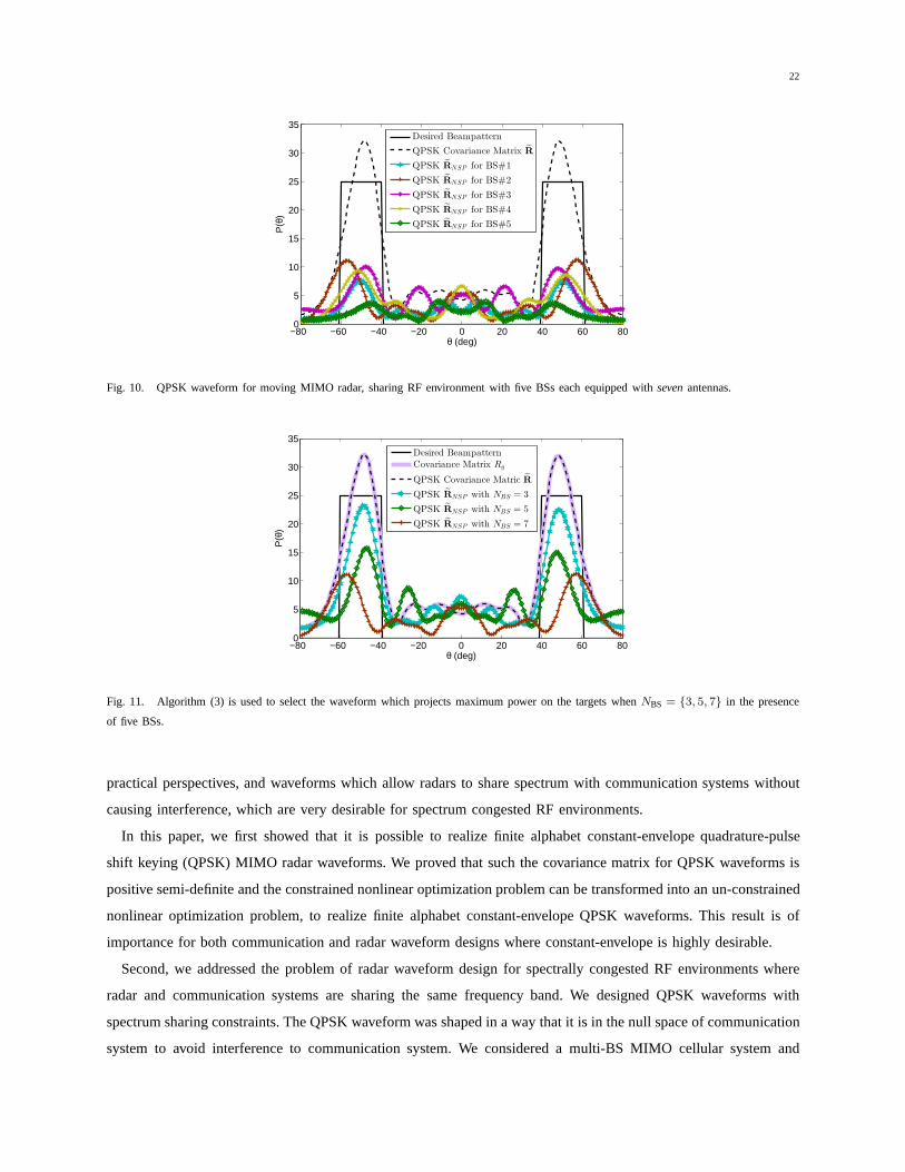
projected waveform was closer to the desired waveform whenNBS ≪ M then whenNBS < M . In Figure 11, we
use Algorithms (1) and (3) to select the waveform which has the least Forbenius norm with respect to the designed
waveform. We apply Algorithms (1) and (3) to the cases whenNBS = {3, 5, 7} and select the waveform which
has minimum Forbenius norm. It can be seen that Algorithm (3)helps us to select waveform for stationary MIMO
radar which results in best performance for radar in terms ofprojected waveform as close as possible to the desired
waveform in addition of meeting spectrum sharing constraints.
IX. CONCLUSION
Waveform design for MIMO radar is an active topic of researchin the signal processing community. This work
addressed the problem of designing MIMO radar waveforms with constant-envelope, which are very desirable from
22
−80 −60 −40 −20 0 20 40 60 800
5
10
15
20
25
30
35
θ (deg)
P(θ
)
Desired Beampattern
QPSK Covariance Matrix R
QPSK RNSP for BS#1
QPSK RNSP for BS#2
QPSK RNSP for BS#3
QPSK RNSP for BS#4
QPSK RNSP for BS#5
Fig. 10. QPSK waveform for moving MIMO radar, sharing RF environment with five BSs each equipped withsevenantennas.
−80 −60 −40 −20 0 20 40 60 800
5
10
15
20
25
30
35
θ (deg)
P(θ
)
Desired Beampattern
Covariance Matrix Rg
QPSK Covariance Matric R
QPSK RNSP with NBS = 3
QPSK RNSP with NBS = 5
QPSK RNSP with NBS = 7
Fig. 11. Algorithm (3) is used to select the waveform which projects maximum power on the targets whenNBS = {3, 5, 7} in the presence
of five BSs.
practical perspectives, and waveforms which allow radars to share spectrum with communication systems without
causing interference, which are very desirable for spectrum congested RF environments.
In this paper, we first showed that it is possible to realize finite alphabet constant-envelope quadrature-pulse
shift keying (QPSK) MIMO radar waveforms. We proved that such the covariance matrix for QPSK waveforms is
positive semi-definite and the constrained nonlinear optimization problem can be transformed into an un-constrained
nonlinear optimization problem, to realize finite alphabetconstant-envelope QPSK waveforms. This result is of
importance for both communication and radar waveform designs where constant-envelope is highly desirable.
Second, we addressed the problem of radar waveform design for spectrally congested RF environments where
radar and communication systems are sharing the same frequency band. We designed QPSK waveforms with
spectrum sharing constraints. The QPSK waveform was shapedin a way that it is in the null space of communication
system to avoid interference to communication system. We considered a multi-BS MIMO cellular system and

23
proposed algorithms for the formation of projection matrices and selection of interference channels. We designed
waveforms for stationary and moving MIMO radar systems. Forstationary MIMO radar we presented an algorithm
for waveform design by considering the spectrum sharing constraints. Our algorithm selected the waveform capable
to project maximum power at the targets. For moving MIMO radar we presented another algorithm for waveform
design by considering spectrum sharing constraints. Our algorithm selected the waveform with the minimum
Forbenius norm with respect to the designed waveform. This metric helped to select the projected waveform closest
to the designed waveform.
APPENDIX A
PRELIMINARIES
This section presents some preliminary results used in the proofs throughout the paper. For proofs of the following
theorems, please see the corresponding references.
Theorem 1. The matrixA ∈ Cn×n is positive semi-definite if and only ifℜ(A) is positive semi-definite [25].
Theorem 2. A necessary and sufficient condition forA ∈ Cn×n to be positive definite is that the Hermitian part
AH =1
2
[A+AH
]
be positive definite [25].
Theorem 3. If A ∈ Cn×n and B ∈ Cn×n are positive semi-definite matrices then the matrixC = A + B is
guaranteed to be positive semi-definite matrix [26].
Theorem 4. If the matrixA ∈ Cn×n is positive semi-definite then thep times Schur product ofA, denoted byAp◦,
will also be positive semi-definite [26].
APPENDIX B
GENERATING CE QPSK RANDOM PROCESSESFROM GAUSSIAN RANDOM VARIABLES
Assuming identically distributed Gaussian RV’sxp, yp, xq and yq that are mapped onto QPSK RV’szp and zq
using
zp =1√2
[sign
(xp√2σ
)+ sign
(yp√2σ
)](60)
zq =1√2
[sign
(xq√2σ
)+ sign
(yq√2σ
)](61)
whereσ2 is the variance of Gaussian RVs. The cross-correlation between QPSK and Gaussian RVs can be derived
as
E{zpz∗q} =1
2E
[{sign
( xp√2σ
)+ sign
( yp√2σ
)}{sign
( xq√2σ
)+ sign
( yq√2σ
)}]· (62)
24
Using equation (13) we can write the above equation as
E{zpz∗q} = E
{sign
( xp√2σ
)sign
( xq√2σ
)}+ E
{sign
( yp√2σ
)sign
( xq√2σ
)}· (63)
The cross-correlation relationship between Gaussian and QPSK RVs can be derived by first considering
E
{sign
( xp√2σ
)sign
( xq√2σ
)}=
∞∫
−∞
∞∫
−∞
[sign
( xp√2σ
)× sign
( xq√2σ
)p(xp, xq, ρxpxq
)
]dxp dxq (64)
wherep(xp, xq, ρxpxq) is the joint probability density function ofxp and xq, andρxpxq
=E{xpx
∗
q}σ2 is the cross-
correlation coefficient ofxp andxq . Using Hermite polynomials [27], the above double integralcan be transformed
as in [7]. Thus,
E
{sign
( xp√2σ
)sign
( xq√2σ
)}=
∞∑
n=0
ρnxpxq
2πσ22nn!×
∞∫
−∞
sign( xp√
2σ
)ex
2
p/2σ2
Hn
( xp√2σ
)dxp
×∞∫
−∞
sign( xq√
2σ
)ex
2
q/2σ2
Hn
( xq√2σ
)dxq (65)
where
Hn(xm) = (−1)nex2m2
dn
dxnme
−x2m
2 (66)
is the Hermite polynomial. By substitutingxp =xp√2σ
and xq =xq√2σ
, and splitting the limits of integration into
two parts, equation (65) can be simplified as
E
{sign(xp)sign(xq)
}=
∞∑
n=0
ρnxpxq
π2nn!
( ∞∫
0
ex2
p
[Hn(xp)−Hn(−xp)
]dxp
)2
· (67)
UsingHn(−xp) = (−1)nHn(xp) [28], equation (67) can be written as
E
{sign(xp)sign(xq)
}=
∞∑
n=0
ρnxpxq
π2nn!
( ∞∫
0
ex2
pHn(xp)(1− (−1)n
)dxp
)2
· (68)
The above equation is non-zero for oddn only, therefore, we can rewrite it as
E
{sign(xp)sign(xq)
}=
∞∑
n=0
ρ2n+1xpxq
π22n(2n+ 1)!
( ∞∫
0
ex2
pH2n+1(xp) dxp
)2
· (69)
Then using∞∫0
ex2
pH2n+1(xp) dxp = (−1)n (2n)!n! from [28], we can write equation (69) as
E
{sign
( xp√2σ
)sign
( xq√2σ
)}=
∞∑
n=0
ρ2n+1xpxq
π22n(2n+ 1)!
((−1)n
2n!
n!
)2
=2
π
[ρxpxq
+ρ3xpxq
2 · 3 +1 · 3ρ5xpxq
2 · 4 · 5 +1 · 3 · 5ρ7xpxq
2 · 4 · 6 · 7 + · · ·]
=2
πsin−1
(E{xpxq}
)(70)

25
In equation (64), we expanded the first part of equation (63).Now, similarly expanding the second part of equation
(63), i.e.,
E
{sign
( yp√2σ
)sign
( xq√2σ
)}=
∞∫
−∞
∞∫
−∞
[sign
( yp√2σ
)sign
( xq√2σ
)p(yp, xq, ρypxq
)
]dyp dxq (71)
wherep(yp, xq, ρypxq) is the joint probability density function ofyp and xq, andρypxq
=E{ypx∗
q}σ2 is the cross-
correlation coefficient ofyp and xq . Using Hermite polynomials, equation (66), we can write equation (71) as
E
{sign
( yp√2σ
)sign
( xq√2σ
)}=
∞∑
n=0
ρnypxq
2πσ22nn!×
∞∫
−∞
sign( yp√
2σ
)× ey
2
p/2σ2
Hn
( yp√2σ
)dyp
×∞∫
−∞
sign( xq√
2σ
)ex
2
q/2σ2
Hn
( xq√2σ
)dxq. (72)
By substitutingyp =yp√2σ
and xq =xq√2σ
, and splitting the limits of integration into two parts, equation (72) can
be simplified as
E
{sign(yp)sign(xq)
}=
∞∑
n=0
ρnypxq
π2nn!
( ∞∫
0
ey2
p
[Hn(yp)−Hn(−yp)
]dyp
)2
· (73)
UsingHn(−yp) = (−1)nHn(yp), above equation can be written as
E
{sign(yp)sign(xq)
}=
∞∑
n=0
ρnypxq
π2nn!
( ∞∫
0
ey2
pHn(yp)(1− (−1)n
)dyp
)2
· (74)
The above equation is non-zero for oddn only, therefore, we can rewrite it as
E
{sign(yp)sign(xq)
}=
∞∑
n=0
ρ2n+1ypxq
π22n(2n+ 1)!
( ∞∫
0
ey2
pH2n+1(yp) dyp
)2
· (75)
Then using∞∫0
ey2
pH2n+1(yp) dyp = (−1)n (2n)!n! , we can write equation (75) as
E
{sign
( yp√2σ
)sign
( xq√2σ
)}=
∞∑
n=0
ρ2n+1ypxq
π22n(2n+ 1)!
((−1)n
2n!
n!
)2
=2
π
[ρypxq
+ρ3ypxq
2 · 3 +1 · 3ρ5ypxq
2 · 4 · 5 +1 · 3 · 5ρ7ypxq
2 · 4 · 6 · 7 + · · ·]
=2
πsin−1
(E{ypxq}
)· (76)
Combining equations (70) and (76), gives us the cross-correlation of equation (63) as
E{zpzq} =2
π
[sin−1
(E{xpxq}
)+ sin−1
(E{ypxq}
)]· (77)

26
APPENDIX C
PROOFS
Proof of Lemma 1:To prove Lemma 1, we note that the real part ofRg is Rg which is positive semi-definite
by definition, thus, by Theorem 1, the complex covariance matrix Rg is also positive semi-definite.
Proof of Lemma 2:To prove Lemma 2, we can individually expand the sum,sin−1(ℜ(Rg)
)+ sin−1
(ℑ(Rg)
),
using Taylor series, i.e., first expandingsin−1(ℜ(Rg)
)
sin−1 (ℜ(Rg)) = ℜ(Rg) +1
2 · 3ℜ(Rg)3◦ +
1 · 32 · 4 · 5ℜ(Rg)
5◦ +
1 · 3 · 52 · 4 · 6 · 7ℜ(Rg)
7◦ + · · · (78)
Then using Theorem 3, each term or matrix, on the right hand side, is positive semi-definite, since,ℜ(Rg) is
positive semi-definite by definition. Moreover,sin−1 (ℜ(Rg)) is also positive semi-definite since its a sum of
positive semi-definite matrices, this follows from Theorem1.
Similarly, expanding sin−1 (ℑ(Rg)) as
sin−1 (ℑ(Rg)) = [ℑ(Rg) +1
2 · 3ℑ(Rg)3◦ +
1 · 32 · 4 · 5ℑ(Rg)
5◦ +
1 · 3 · 52 · 4 · 6 · 7ℑ(Rg)
7◦ + · · · ] (79)
Now, R is positive semi-definite since real part of it is positive semidefinite, from equation (78) and Theorem 4.
REFERENCES
[1] J. Li and P. Stoica,MIMO Radar Signal Processing. Wiley-IEEE Press, 2008.
[2] A. M. Haimovich, R. S. Blum, and L. J. Cimini, “MIMO Radar with Widely Separated Antennas,”IEEE Signal Processing Magazine,
vol. 25, no. 1, pp. 116–129, 2008.
[3] J. Li and P. Stoica, “MIMO radar with colocated antennas,” IEEE Signal Processing Magazine, vol. 24, no. 5, pp. 106–114, 2007.
[4] J. Tan and G. Stuber, “Constant envelope multi-carrier modulation,” in MILCOM 2002. Proceedings, vol. 1, pp. 607–611 vol.1, Oct 2002.
[5] S. Thompson, A. Ahmed, J. Proakis, J. Zeidler, and M. Geile, “Constant envelope OFDM,”IEEE Transactions on Communications, vol. 56,
pp. 1300–1312, August 2008.
[6] P. Stoica, J. Li, and X. Zhu, “Waveform synthesis for diversity-based transmit beampattern design,”IEEE Transactions on Signal Processing,
vol. 56, pp. 2593–2598, June 2008.
[7] S. Ahmed, J. S. Thompson, Y. R. Petillot, and B. Mulgrew, “Finite alphabet constant-envelope waveform design for MIMO radar,” IEEE
Transactions on Signal Processing, vol. 59, no. 11, pp. 5326–5337, 2011.
[8] S. Sodagari and A. Abdel-Hadi, “Constant envelope radarwith coexisting capability with LTE communication systems,” under submission.
[9] The Presidents Council of Advisors on Science and Technology (PCAST), “Realizing the full potential of government-held spectrum to
spur economic growth,” July 2012.
[10] Federal Communications Commission (FCC), “FCC proposes innovative small cell use in 3.5 GHz band.” Online:
http://www.fcc.gov/document/fcc-proposes-innovative-small-cell-use-35-ghz-band, December 12, 2012.
[11] H. Shajaiah, A. Khawar, A. Abdel-Hadi, and T. C. Clancy,“Using resource allocation with carrier aggregation for spectrum sharing between
radar and 4G-LTE cellular system,” inIEEE DySPAN, 2014.
[12] M. Ghorbanzadeh, A. Abdelhadi, and C. Clancy, “A utility proportional fairness resource allocation in spectrallyradar-coexistent cellular
networks,” inMilitary Communications Conference (MILCOM), 2014.
[13] A. Khawar, A. Abdelhadi, and T. C. Clancy, “On The Impactof Time-Varying Interference-Channel on the Spatial Approach of Spectrum
Sharing between S-band Radar and Communication System,” inMilitary Communications Conference (MILCOM), 2014.
[14] D. Fuhrmann and G. San Antonio, “Transmit beamforming for MIMO radar systems using signal cross-correlation,”IEEE Transactions
on Aerospace and Electronic Systems, vol. 44, pp. 171–186, January 2008.
27
[15] T. Aittomaki and V. Koivunen, “Signal covariance matrix optimization for transmit beamforming in MIMO radars,” inin Proc. of the
Forty-First Asilomar Conference on Signals, Systems and Computers (ASILOMAR), pp. 182–186, Nov 2007.
[16] P. Gong, Z. Shao, G. Tu, and Q. Chen, “Transmit beampattern design based on convex optimization for{MIMO} radar systems,”Signal
Processing, vol. 94, no. 0, pp. 195 – 201, 2014.
[17] G. Hua and S. Abeysekera, “MIMO radar transmit beampattern design with ripple and transition band control,”IEEE Transactions on
Signal Processing, vol. 61, pp. 2963–2974, June 2013.
[18] S. Sodagari, A. Khawar, T. C. Clancy, and R. McGwier, “A projection based approach for radar and telecommunication systems coexistence,”
in IEEE Global Communications Conference (GLOBECOM), 2012.
[19] A. Khawar, A. Abdel-Hadi, T. C. Clancy, and R. McGwier, “Beampattern analysis for MIMO radar and telecommunicationsystem
coexistence,” inIEEE International Conference on Computing, Networking and Communications, Signal Processing for Communications
Symposium (ICNC’14 - SPC), 2014.
[20] A. Khawar, A. Abdel-Hadi, and T. C. Clancy, “MIMO radar waveform design for coexistence with cellular systems,” in2014 IEEE
International Symposium on Dynamic Spectrum Access Networks: SSPARC Workshop (IEEE DySPAN 2014 - SSPARC Workshop), (McLean,
USA), Apr. 2014.
[21] A. Khawar, A. Abdel-Hadi, and T. C. Clancy, “Spectrum sharing between S-band radar and LTE cellular system: A spatial approach,”
in 2014 IEEE International Symposium on Dynamic Spectrum Access Networks: SSPARC Workshop (IEEE DySPAN 2014 - SSPARC
Workshop), (McLean, USA), Apr. 2014.
[22] D. Tse and P. Viswanath,Fundamentals of Wireless Communication. Cambridge University Press, 2005.
[23] S. Ahmed, J. Thompson, Y. Petillot, and B. Mulgrew, “Unconstrained synthesis of covariance matrix for MIMO radar transmit beampattern,”
IEEE Transactions on Signal Processing, vol. 59, pp. 3837–3849, aug. 2011.
[24] A. Hyvarinen, J. Karhunen, and E. Oja,Independent Component Analysis. Wiley-Interscience, 2001.
[25] D. S. Bernstein,Matrix Mathematics: Theory, Facts, and Formulas. Princeton University Press, second ed., 2009.
[26] R. A. Horn and C. R. Johnson,Matrix Analysis. Cambridge, U.K.: Cambridge University Press, 1985.
[27] J. Brown, Jr., “On the expansion of the bivariate gaussian probability density using results of nonlinear theory (corresp.),”IEEE Transactions
on Information Theory, vol. 14, pp. 158–159, Sept. 1968.
[28] A. De Maio, S. De Nicola, A. Farina, and S. Iommelli, “Adaptive detection of a signal with angle uncertainty,”IET Radar, Sonar Navigation,
vol. 4, pp. 537–547, August 2010.