1. Reliability 2. - Imperial College Londonnucinkis-lab.cc.ic.ac.uk/.../workbook_46/46_1_reliability.pdf · Reliability 2. Quality Control Learning outcomes ... An alternative answer

ContentsContents Reliability and

quality control 1. Reliability

2. Quality Control

Learning outcomes

You will first learn about the importance of the concept of reliability applied to systems and

products. The second Section introduces you to the very important topic of quality control

in production processes. In both cases you will learn how to perform the basic calculations

necessary to use each topic in practice.

Time allocation

You are expected to spend approximately ten hours of independent study on the

material presented in this workbook. However, depending upon your ability to concentrate

and on your previous experience with certain mathematical topics this time may vary

considerably.

1

Reliability�

�

�

�46.1Introduction

Much of the theory of reliability was developed initially for use in the electronics industrywhere components often fail with little if any prior warning. In such cases the hazard functionor conditional failure rate function is constant and any functioning component or system istaken to be ‘as new’ . There are other cases where the conditional failure rate function is timedependent, often proportional to the time that the system or component has been in use. Thefunction may be an increasing function of time (as with random vibrations for example) ordecreasing with time (as with concrete whose strength, up to a point, increases with time). Ifwe can develop a lifetime model, we can use it to plan such things as maintenance and partreplacement schedules, whole system replacements and reliability testing schedules.

�

�

�

�

PrerequisitesBefore starting this Section you should . . .

① be familiar with the results and conceptsmet in the study of probability

② understand and be able to use continuousprobability distributions

Learning OutcomesAfter completing this Section you should beable to . . .

✓ appreciate the importance of lifetime dis-tributions

✓ understand how to complete reliabilitycalculations for simple systems

✓ understand the relationship between theWeibull distribution and the exponentialdistribution

1. Reliability

Lifetime DistributionsFrom an engineering point of view, the ability to predict the lifetime of a whole system ora system component is very important. Such lifetimes can be predicted using a statisticalapproach using appropriate distributions. Common examples of structures whose lifetimes weneed to know are airframes, bridges, oil rigs and at a simpler, less catastrophic level, systemcomponents such as cycle chains, engine timing belts and components of electronic systemssuch as televisions and computers. If we can develop a lifetime model, we can use it to plansuch things as maintenance and part replacement schedules, whole system replacements andreliability testing schedules.

We start by looking at the length of use of a system or component prior to failure (the age priorto failure) and from this develop a definition of reliability. Lifetime distributions are functionsof time and may be expressed as probability density functions and so we may write

P (t) =

∫ t

0

p(t)dt

This represents the probability that the system or component fails anywhere between 0 and t.Hence, the probability that a system or component will fail only after time t may be written as

R(t) = 1 − P (t)

The function R(t) is usually called the reliability function.

In practice engineers (and others!) are often interested in the so-called hazard function orconditional failure rate function which gives the probability that a system or component failsafter it has been in use for a given time. This function may be defined as

H(t) = lim∆t→o

(P (failure in the interval (t, t + ∆t))/∆t

P (survival up to time t)

)

=1

R(t)lim

∆t→o

(P (t + ∆t) − P (t)

∆t

)

=1

R(t)

d

dtP (t)

=p(t)

R(t)

This gives the conditional failure rate function as

H(t) = lim∆t→o

∫ t+∆t

t

p(t)dt/(∆t)

R(t)

=p(t)

R(t)

Essentially we are describing the rate of failure per unit time for (say) mechanical or electricalcomponents which have already been in service for a given time.

3 HELM (VERSION 1: April 14, 2004): Workbook Level 146.1: Reliability

A graph of H(t) often shows a high initial failure rate followed by a period of relative reliabilityfollowed by a period of increasingly high failure rates as a system or component ages. A typicalgraph (sometimes called a bathtub graph) is shown below.

H(t)

0 t

Early life andrandom failure Useful life and random failure

End of life andrandom failure

Note that ‘early life and random failure’ includes failure due to defects being present and that‘end of life and random failure’ includes failure due to ageing.The reliability of a system or component may be defined as the probability that the system orcomponent functions for a given time, that is, the probability that it will fail only after the giventime. Put another way, R(t) is the probability that the system or component is still functioningat time t.

The Exponential Distribution

We have already met the exponential distribution in the form

f(t) = λe−λt, t ≥ 0

However, one of the simplest distributions describing failure is the exponential distribution

p(t) =1

µe−t/µ, t ≥ 0

where, (in this case) µ is the mean time to failure. One property of this distribution is thatthe hazard function is a constant independent of time - the ‘good as new’ syndrome mentionedabove.

To show that the probability of failure is independent of age consider the following.

P (t) =

∫ t

0

1

µe−t/µdt =

1

µ

[−µe−t/µ

]t

0= 1 − e−t/µ

Hence the reliability (given that the total area under the curve P (t) = 1 − e−t/µ is unity) is

R(t) = 1 − P (t) = e−t/µ

Hence, the hazard function or conditional failure rate function H(t) is given by

H(t) =p(t)

R(t)=

1µe−t/µ

e−t/µ=

1

µ

which is a constant independent of time.

HELM (VERSION 1: April 14, 2004): Workbook Level 146.1: Reliability

4

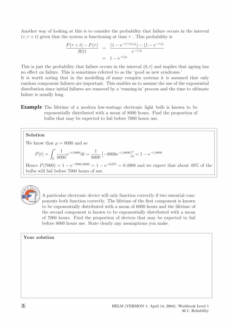
Another way of looking at this is to consider the probability that failure occurs in the interval(τ, τ + t) given that the system is functioning at time τ . This probability is

F (τ + t) − F (τ)

R(t)=

(1 − e−(τ+t)/µ) − (1 − e−τ/µ

e−τ/µ

= 1 − e−t/µ

This is just the probability that failure occurs in the interval (0, t) and implies that ageing hasno effect on failure. This is sometimes referred to as the ‘good as new syndrome.’It is worth noting that in the modelling of many complex systems it is assumed that onlyrandom component failures are important. This enables us to assume the use of the exponentialdistribution since initial failures are removed by a ‘running-in’ process and the time to ultimatefailure is usually long.

Example The lifetime of a modern low-wattage electronic light bulb is known to beexponentially distributed with a mean of 8000 hours. Find the proportion ofbulbs that may be expected to fail before 7000 hours use.

Solution

We know that µ = 8000 and so

P (t) =

∫ t

0

1

8000e−t/8000dt =

1

8000

[−8000e−t/8000

]t

0= 1 − e−t/8000

Hence P (7000) = 1 − e−7000/8000 = 1 − e−0.675 = 0.4908 and we expect that about 49% of thebulbs will fail before 7000 hours of use.

A particular electronic device will only function correctly if two essential com-ponents both function correctly. The lifetime of the first component is knownto be exponentially distributed with a mean of 6000 hours and the lifetime ofthe second component is known to be exponentially distributed with a meanof 7000 hours. Find the proportion of devices that may be expected to failbefore 8000 hours use. State clearly any assumptions you make.

Your solution


Theassumptionmadeisthatthecomponentsoperateindependently.

ForthefirstcomponentP(t)=1−e−t/6000sothatP(8000)=1−e−8000/6000

=1−e−4/3=0.7364

ForthesecondcomponentP(t)=1−e−t/7000sothatP(8000)=1−e−8000/7000

=0.6811

Theprobabilitythatthedevicewillcontinuetofunctionafter8000hoursuseisgivenbyanexpressionoftheform

P(A∪B)=P(A)+P(B)−P(A∩B)

Hencetheprobabilitythatthedevicewillcontinuetofunctionafter8000houruseis

0.7364+0.6811−0.7364×0.6811=0.916

andweexpectjustunder92%ofthedevicestofailbefore8000hoursuse.

An alternative answer may be obtained more directly by using the reliability function R(t).

Theassumptionmadeisthatthecomponentsoperateindependently.

ForthefirstcomponentR(t)=e−t/6000sothatR(8000)=e−8000/6000

=e−4/3=0.2636

ForthesecondcomponentR(t)=e−t/7000sothatR(8000)=e−8000/7000

=0.3189

Theprobabilitythatthedevicewillcontinuetofunctionafter8000houruseisgivenby

0.2636×0.3189=0.0841

Hencetheprobabilitythatthedevicewillfailbefore8000hoursuseis

1−0.0841=0.916

andweexpectjustunder92%ofthedevicestofailbefore8000hoursuse.

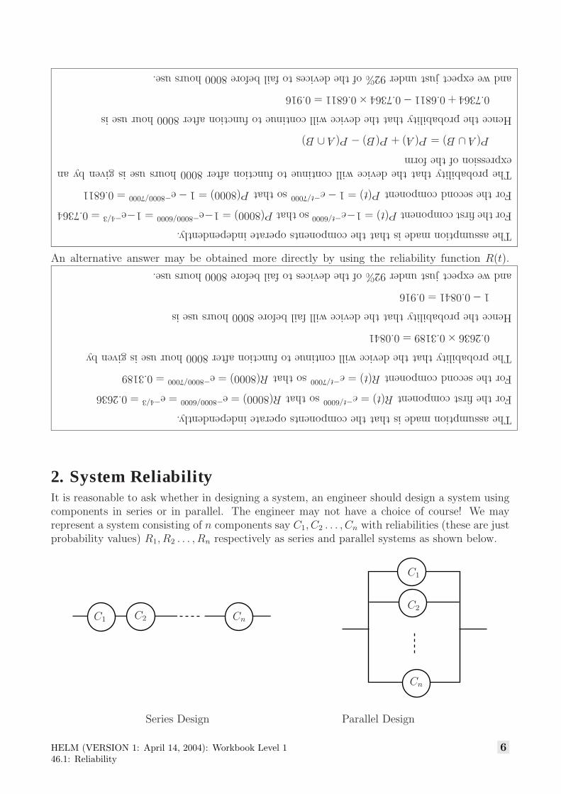
2. System ReliabilityIt is reasonable to ask whether in designing a system, an engineer should design a system usingcomponents in series or in parallel. The engineer may not have a choice of course! We mayrepresent a system consisting of n components say C1, C2 . . . , Cn with reliabilities (these are justprobability values) R1, R2 . . . , Rn respectively as series and parallel systems as shown below.

C1

C1 C2 Cn

C2

Cn

Series Design Parallel Design


6

With a series design, the system will fail if any component fails. With a parallel design, thesystem will work as long as any component works.

Assuming that the components are independent, we can express the reliability of the seriesdesign as

RSeries = R1 × R2 × · · · × Rn

simply by multiplying the probabilities.

Since each reliability value is less than one, we may conclude that a series design is less reliablethan its least reliable component.

Similarly (although by no means as clearly!), we can express the reliability of the parallel designas

RParallel = 1 − (1 − R1)(1 − R2) . . . (1 − Rn)

The derivation of this result is illustrated in the second of the worked examples below for thecase n = 3 . In this case, the algebra involved in fairly straightforward. We can conclude thatthe parallel design is at least as reliable as the most reliable component.

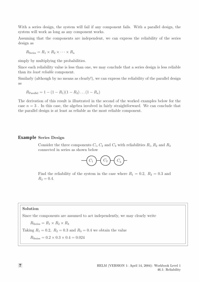
Example Series Design

Consider the three components C1, C2 and C3 with reliabilities R1, R2 and R3

connected in series as shown below

C1 C2 C

Find the reliability of the system in the case where R1 = 0.2, R2 = 0.3 andR3 = 0.4.

Solution

Since the components are assumed to act independently, we may clearly write

RSeries = R1 × R2 × R3

Taking R1 = 0.2, R2 = 0.3 and R3 = 0.4 we obtain the value

RSeries = 0.2 × 0.3 × 0.4 = 0.024


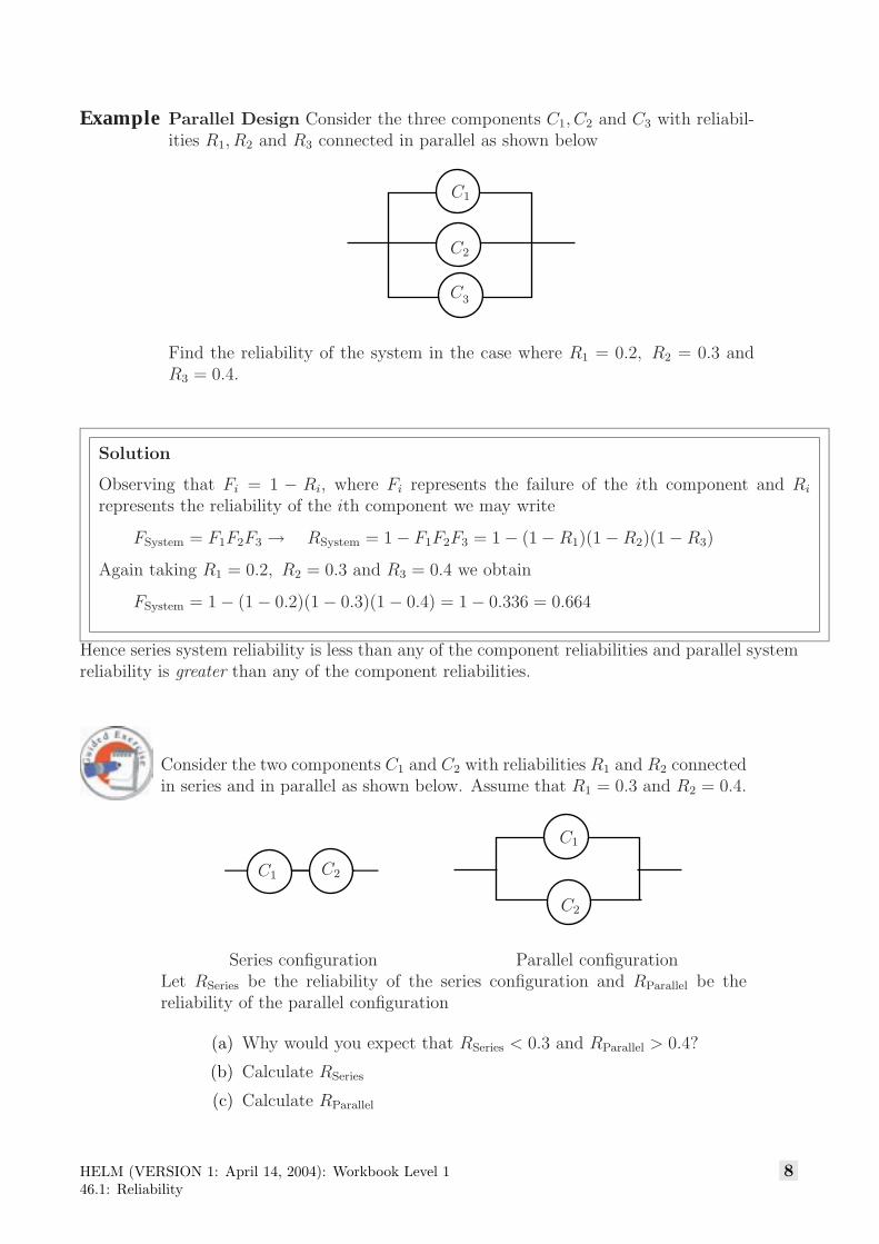
Example Parallel Design Consider the three components C1, C2 and C3 with reliabil-ities R1, R2 and R3 connected in parallel as shown below

C1

C2

C

Find the reliability of the system in the case where R1 = 0.2, R2 = 0.3 andR3 = 0.4.

Solution

Observing that Fi = 1 − Ri, where Fi represents the failure of the ith component and Ri

represents the reliability of the ith component we may write

FSystem = F1F2F3 → RSystem = 1 − F1F2F3 = 1 − (1 − R1)(1 − R2)(1 − R3)

Again taking R1 = 0.2, R2 = 0.3 and R3 = 0.4 we obtain

FSystem = 1 − (1 − 0.2)(1 − 0.3)(1 − 0.4) = 1 − 0.336 = 0.664

Hence series system reliability is less than any of the component reliabilities and parallel systemreliability is greater than any of the component reliabilities.

Consider the two components C1 and C2 with reliabilities R1 and R2 connectedin series and in parallel as shown below. Assume that R1 = 0.3 and R2 = 0.4.

C1 C2

C1

C2

Series configuration Parallel configurationLet RSeries be the reliability of the series configuration and RParallel be thereliability of the parallel configuration

(a) Why would you expect that RSeries < 0.3 and RParallel > 0.4?

(b) Calculate RSeries

(c) Calculate RParallel


8

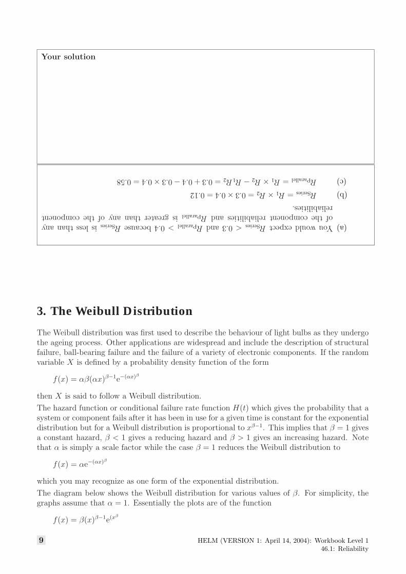
Your solution

(a)YouwouldexpectRSeries<0.3andRParallel>0.4becauseRSeriesislessthananyofthecomponentreliabilitiesandRParallelisgreaterthananyofthecomponentreliabilities.

(b)RSeries=R1×R2=0.3×0.4=0.12

(c)RParallel=R1×R2−R1R2=0.3+0.4−0.3×0.4=0.58

3. The Weibull Distribution

The Weibull distribution was first used to describe the behaviour of light bulbs as they undergothe ageing process. Other applications are widespread and include the description of structuralfailure, ball-bearing failure and the failure of a variety of electronic components. If the randomvariable X is defined by a probability density function of the form

f(x) = αβ(αx)β−1e−(αx)β

then X is said to follow a Weibull distribution.

The hazard function or conditional failure rate function H(t) which gives the probability that asystem or component fails after it has been in use for a given time is constant for the exponentialdistribution but for a Weibull distribution is proportional to xβ−1. This implies that β = 1 givesa constant hazard, β < 1 gives a reducing hazard and β > 1 gives an increasing hazard. Notethat α is simply a scale factor while the case β = 1 reduces the Weibull distribution to

f(x) = αe−(αx)β

which you may recognize as one form of the exponential distribution.

The diagram below shows the Weibull distribution for various values of β. For simplicity, thegraphs assume that α = 1. Essentially the plots are of the function

f(x) = β(x)β−1e(xβ


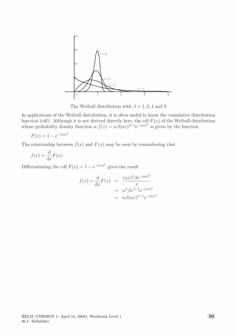
β = 1

β = 2

β = 4

β = 8

1

2

3

0 1 2 3 4

4

The Weibull distribution with β = 1, 2, 4 and 8

In applications of the Weibull distribution, it is often useful to know the cumulative distributionfunction (cdf). Although it is not derived directly here, the cdf F (x) of the Weibull distributionwhose probability density function is f(x) = αβ(αx)β−1e−(αx)β

is given by the function

F (x) = 1 − e−(αx)β

The relationship between f(x) and F (x) may be seen by remembering that

f(x) =d

dxF (x)

Differentiating the cdf F (x) = 1 − e−(αx)β

gives the result

f(x) =d

dxF (x) =

(αx)ββe−(αx)β

x

= αββxβ−1e−(αx)β

= αβ(αx)β−1e−(αx)β


10

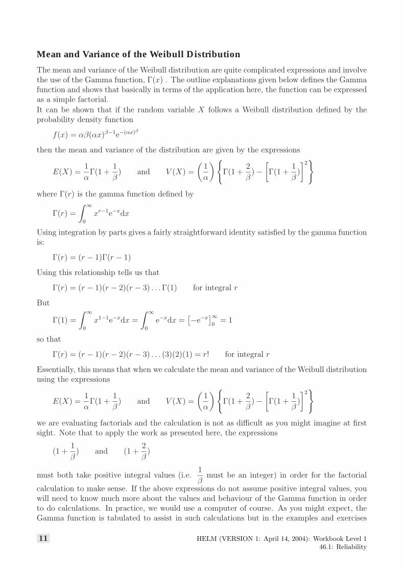
Mean and Variance of the Weibull Distribution

The mean and variance of the Weibull distribution are quite complicated expressions and involvethe use of the Gamma function, Γ(x) . The outline explanations given below defines the Gammafunction and shows that basically in terms of the application here, the function can be expressedas a simple factorial.

It can be shown that if the random variable X follows a Weibull distribution defined by theprobability density function

f(x) = αβ(αx)β−1e−(αx)β

then the mean and variance of the distribution are given by the expressions

E(X) =1

αΓ(1 +

1

β) and V (X) =

(1

α

) {Γ(1 +

2

β) −

[Γ(1 +

1

β)

]2}

where Γ(r) is the gamma function defined by

Γ(r) =

∫ ∞

0

xr−1e−xdx

Using integration by parts gives a fairly straightforward identity satisfied by the gamma functionis:

Γ(r) = (r − 1)Γ(r − 1)

Using this relationship tells us that

Γ(r) = (r − 1)(r − 2)(r − 3) . . . Γ(1) for integral r

But

Γ(1) =

∫ ∞

0

x1−1e−xdx =

∫ ∞

0

e−xdx =[−e−x

]∞0

= 1

so that

Γ(r) = (r − 1)(r − 2)(r − 3) . . . (3)(2)(1) = r! for integral r

Essentially, this means that when we calculate the mean and variance of the Weibull distributionusing the expressions

E(X) =1

αΓ(1 +

1

β) and V (X) =

(1

α

) {Γ(1 +

2

β) −

[Γ(1 +

1

β)

]2}

we are evaluating factorials and the calculation is not as difficult as you might imagine at firstsight. Note that to apply the work as presented here, the expressions

(1 +1

β) and (1 +

2

β)

must both take positive integral values (i.e.1

βmust be an integer) in order for the factorial

calculation to make sense. If the above expressions do not assume positive integral values, youwill need to know much more about the values and behaviour of the Gamma function in orderto do calculations. In practice, we would use a computer of course. As you might expect, theGamma function is tabulated to assist in such calculations but in the examples and exercises


set in this booklet, the values of1

βwill always be integral.

Example The main drive shaft of a pumping engine runs in two bearings whose behaviourfollows a Weibull distribution with random variable X and parameters α =0.0002 and β = 0.5.

(a) Find the expected time that a single bearing runs before failure.

(b) Find the probability that any one bearing lasts at least 8000 hours.

(c) Find the probability that both bearings last at least 6000 hours.

Solution

(a) We know that E(X) =1

αΓ(1 +

1

β) = 5000 × Γ(1 + 2) = 5000 × 2 = 10000 hours.

(b) We require P (X > 8000) , this is given by the calculation:

P (X > 8000) = 1 − P (8000) = 1 − (1 − e−(0.0002×8000)0.5

)

= e−(0.0002×8000)0.5

= e−1.265

= 0.282

(c) Assuming that the bearings wear independently, the probability that both bearingslast at least 6000 hours is given by [P (X > 6000)]2. But P (X > 6000) is given bythe calculation

P (X > 6000) = 1 − P (6000) = 1 − (1 − e−(0.0002×6000)0.5

)

= 0.335

so that the probability that both bearings last at least 6000 hours is given by

[P (X > 6000)]2 = 0.3352 = 0.112

A shaft runs in four roller bearings the lifetime of each of which follows aWeibull distribution with parameters α = 0.0001 and β = 1/3.

(a) Find the mean life of a bearing.

(b) Find the variance of the life of bearing.

(c) Find the probability that all four bearings last at least 50000 hours.State clearly any assumptions you make when determining thisprobability.


12

Your solution

(a)WeknowthatE(X)=1

αΓ(1+

1

β)=10000×Γ(1+3)=60000×2=10000hours.

(b)WeknowthatV(X)=

(1

α

){Γ(1+

2

β)−

[Γ(1+

1

β

]2}sothat

V(X)=(10000)2{Γ(1+6)−(Γ(1+3)]

2}

=(10000)2{Γ(7)−[Γ(4)]

2}

=(10000)2{6!−(3!)

2}

=684(10000)2

(c)Theprobabilitythatonebearingwilllastatleast50000hoursisgivenbythecal-culation

P(X>50000)=1−P(50000)

=1−(1−e−(0.0001×50000)0.5

)

=e−50.5

=0.107

Assumingthatthefourbearingshaveindependentdistributions,theprobabilitythatallfourbearingslastatleast50000hoursis(0.107)

4=0.0001


Exercises

1. The lifetimes in hours of certain machines have Weibull distributions with probabilitydensity function

f(t) =

{0 (t < 0)

αβ(αt)β−1 exp{−(αt)β} (t ≥ 0)

(a) Verify that ∫ t

0

αβ(αu)β−1 exp{−(αu)β}.du = 1 − exp{−(αt)β}.

(b) Write down the distribution function of the lifetime.

(c) Find the probability that a particular machine is still working after 500 hours of useif α = 0.001 and β = 2.

(d) In a factory, n of these machines are installed and started together. Assuming thatfailures in the machines are independent, find the probability that all of the machinesare still working after t hours and hence find the probability density function of thetime till the first failure among the machines.

2. If the lifetime distribution of a machine has hazard function h(t), then we can find the reli-ability function R(t) as follows. First we find the “cumulative hazard function” H(t) using

H(t) =

∫ t

0

h(t).dt. then the reliability is R(t) = e−H(t).

(a) Starting with R(t) = exp{−H(t)}, work back to the hazard function and henceconfirm the method of finding the reliability from the hazard.

(b) A lifetime distribution has hazard function h(t) = θ0 + θ1t + θ2t2.

Find (i) the reliability function. (ii) the probability density function.

(c) A lifetime distribution has hazard function h(t) =1

t + 1.

Find (i) the reliability function. (ii) the probability density function.(iii) the median.What happens if you try to find the mean?

(d) A lifetime distribution has hazard function h(t) =ρθ

ρt + 1, where ρ > 0 and θ > 1.

Find (i) the reliability function. (ii) the probability density function.

(iii) the median. (iv) the mean.

3. A machine has n components, the lifetimes of which are independent. However the wholemachine will fail if any component fails. The hazard functions for the components areh1(t), . . . , hn(t). Show that the hazard function for the machine is

∑ni=1 hi(t).

4. Suppose that the lifetime distributions of the components in Question ?? are Weibull dis-tributions with scale parameters ρ1, . . . , ρn and a common index (i.e. “shape parameter”)γ so that the hazard function for component i is γρi(ρit)

γ−1. Find the lifetime distributionfor the machine.


14

Exercises Continued5. (Difficult). Show that, if T is a Weibull random variable with hazard function γρ(ρt)γ−1,

(a) the median is M(T ) = ρ−1(log 2)1/γ,

(b) the mean is E(T ) = ρ−1Γ(1 + γ−1) and

(c) the variance is var(T ) = ρ−2{Γ(1 + 2γ−1) − [Γ(1 + γ−1)]2}.

Note that Γ(r) =∫ ∞

0xr−1e−x.dx. In the integrations it is helpful to use the substitution u =

(ρt)γ.


Answers

1.

(a)d

du[−exp{−(αu)

β}]

so

∫t

0

αβ(αu)β−1

exp{−(αu)β}.du=[−exp{−(αu)

β}]

t0=1−exp{−(αt)

β}.

(b)ThedistributionfunctionisF(t)=1−exp{−(αt)β}.

(c)R(500)=exp{−(0.001×500)

2}=0.7788.

(d)Theprobabilitythatallofthemachinesarestillworkingafterthoursis

Rn(t)=[R(t)]n

=exp{−(αt)nβ}.

HencethetimetothefirstfailurehasaWeibulldistributionwithβreplacedbynβ.Thepdfis

fn(t)=

{0(t<0)αnβ(αt)

nβ−1exp{−(αt)

nβ}(t≥0)

2.

(a)Thedistributionfunctionis

F(t)=1−R(t)=1−e−H(t)sothepdfisf(t)=

d

dtF(t)=h(t)e−H(t)

.

Hencethehazardfunctionis

h(t)=f(t)

R(t)=

h(t)e−H(t)

e−H(t)=h(t).

(b)Alifetimedistributionhashazardfunctionh(t)=θ0+θ1t+θ2t2.

i.ReliabilityR(t).

H(t)=[θ0t+θ1t2/2+θ2t

3/3]

t0

=θ0t+θ1t2/2+θ2t

3/3

R(t)=exp{−[θ0t+θ1t2/2+θ2t

3/3]}.

ii.Probabilitydensityfunctionf(t).

F(t)=1−R(t)f(t)=(θ0+θ1t+θ2t2)exp{−[θ0t+θ1t

2/2+θ2t

3/3]}.


16

Continued(c)Alifetimedistributionhashazardfunctionh(t)=1

t+1.

i.ReliabilityfunctionR(t).

H(t)=

∫t

0

1

u+1.du=[log(u+1)]

t0=log(t+1)

R(t)=exp[−H(t)]=1

t+1

ii.Probabilitydensityfunctionf(t).F(t)=1−R(t)f(t)=1

(t+1)2

iii.MedianM.1

M+1=12soM=1.

Tofindthemean:E(T+1)=

∫∞

0

1

t+1.dt

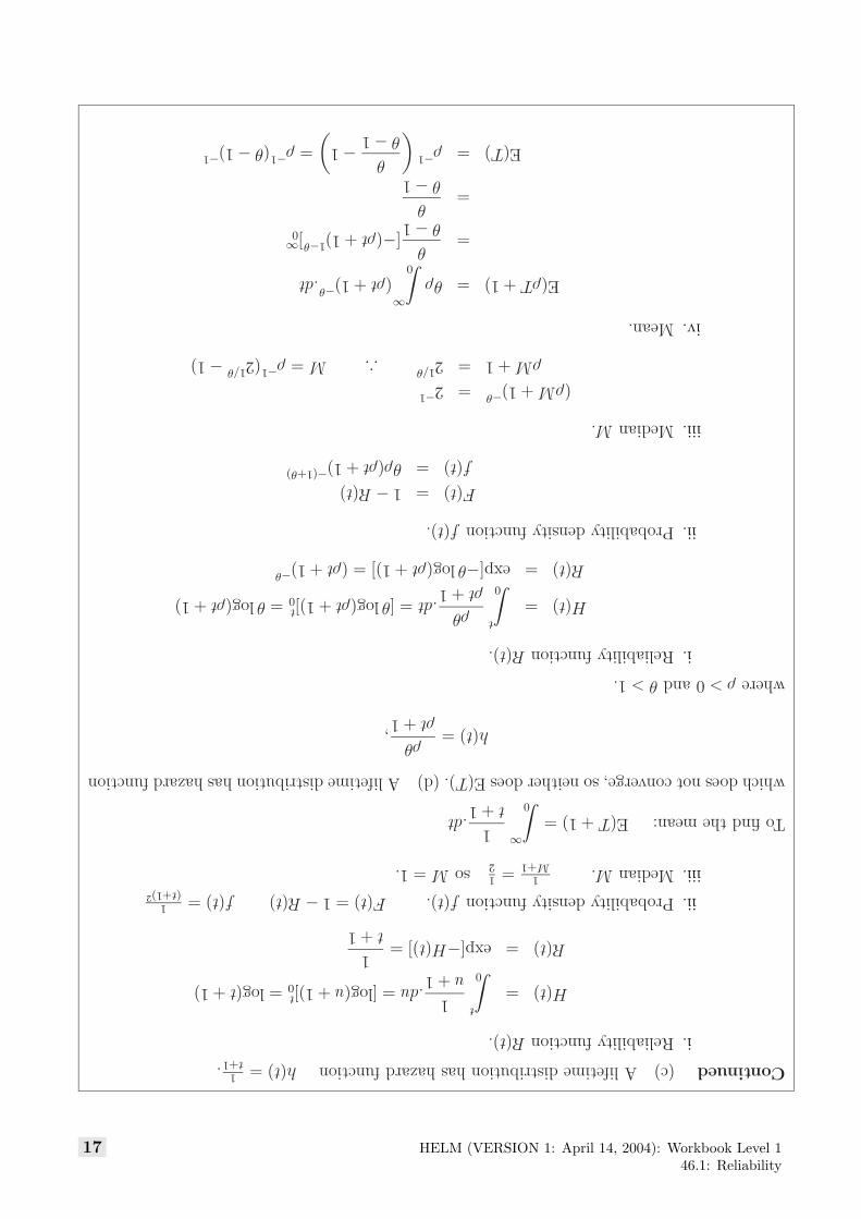
whichdoesnotconverge,soneitherdoesE(T).(d)Alifetimedistributionhashazardfunction

h(t)=ρθ

ρt+1,

whereρ>0andθ>1.

i.ReliabilityfunctionR(t).

H(t)=

∫t

0

ρθ

ρt+1.dt=[θlog(ρt+1)]

t0=θlog(ρt+1)

R(t)=exp[−θlog(ρt+1)]=(ρt+1)−θ

ii.Probabilitydensityfunctionf(t).

F(t)=1−R(t)

f(t)=θρ(ρt+1)−(1+θ)

iii.MedianM.

(ρM+1)−θ=2−1

ρM+1=21/θ

∴M=ρ−1(2

1/θ−1)

iv.Mean.

E(ρT+1)=θρ

∫∞

0

(ρt+1)−θ.dt

=θ

θ−1[−(ρt+1)

1−θ]∞0

=θ

θ−1

E(T)=ρ−1(θ

θ−1−1

)=ρ−1

(θ−1)−1


Continued

4.Foreachcomponent

Hi(t)=

∫t

0

hi(t).dt

Ri(t)=exp{−Hi(t)}

Formachine

R(t)=n∏

i=1

Ri(t)=exp{−n∑

i=1

Hi(t)}

theprobabilitythatallcomponentsarestillworking.

F(t)=1−R(t)

f(t)=exp{−n∑

i=1

Hi(t)}n∑

i=1

Hi(t)

h(t)=f(t)/R(t)=n∑

i=1

hi(t).

5.Foreachcomponent

hi(t)=γρi(ρit)γ−1

Hi(t)=

∫t

0

γρi(ρit)γ−1

.dt=(ρit)γ

Hence,forthemachine,

n∑i=1

Hi(t)=tγ

n∑i=1

ργi

R(t)=exp

(−t

γ

n∑i=1

ργi

)

F(t)=1−R(t)

f(t)=γtγ−1

n∑i=1

ργiexp

(−t

γ

n∑i=1

ργi

)

h(t)=γρ(ρt)γ−1

sowehaveaWeibulldistributionwithindexγandscaleparameterρsuchthat

ργ

=n∑

i=1

ργi.


18

Documents

1. Reliability 2. - Imperial College Londonnucinkis-lab.cc.ic.ac.uk/.../workbook_46/46_1_reliability.pdf · Reliability 2. Quality Control Learning outcomes ... An alternative answer