1 Rigid Network Design Via Submodular Set Function ...€¦1 Rigid Network Design Via Submodular Set Function Optimization Iman Shames, Tyler H. Summers Abstract We consider the problem

1

Rigid Network Design Via Submodular Set

Function OptimizationIman Shames, Tyler H. Summers

Abstract

We consider the problem of constructing networks that exhibit desirable algebraic rigidity properties, which can

provide significant performance improvements for associated formation shape control and localization tasks. We show

that the network design problem can be formulated as a submodular set function optimization problem and propose

greedy algorithms that achieve global optimality or an established near-optimality guarantee. We also consider the

separate but related problem of selecting anchors for sensor network localization to optimize a metric of the error

in the localization solutions. We show that an interesting metric is a modular set function, which allows a globally

optimal selection to be obtained using a simple greedy algorithm. The results are illustrated via numerical examples,

and we show that the methods scale to problems well beyond the capabilities of current state-of-the-art convex

relaxation techniques.

I. INTRODUCTION

Accelerating advances in communication, computation, and sensing technologies are allowing networks of low-

cost interconnected nodes to provide unprecedented data streams about physical processes, and position control

and localization of (mobile sensor) node positions is often required to meaningfully interpret and utilize the data.

There are several broad categories of measurement techniques that can be used for position localization and control,

including angle of arrival, received signal strength profiling, and distance related measurements. In this paper, we

will focus on distance-based scenarios in the plane; however, similar results can be obtained for other types of

measurements and in higher dimensions.

The application of rigid graph theory to distanced-based motion control in mobile robot formations and localization

problems in sensor networks has been the focus of many recent studies [1]–[11]. In formation shape control

problems, the literature is focused on characterizing rigid graph properties that allow distributed control of any

desired configuration [1]–[3] and associated control law design [4]–[6]. Similarly, the sensor network localization

literature has focused on characterizing rigid graph properties that allow unique localization solutions [7], [8], [10],

[12]–[14] and associated localization algorithms [9]–[11].

I. Shames is with the Department of Electrical and Electronic Engineering, University of Melbourne, Australia. T. H. Sum-

mers is with the Department of Mechanical Engineering, University of Texas at Dallas. [email protected],

[email protected].

September 15, 2015 DRAFT

2

While many aspects of distanced-based motion control and localization problems have been studied in detail,

very few papers consider design of the network itself. In particular, the distances to be actively controlled in a

formation control problem or the distance measurements in a localization problem are typically taken as given.

However, a network designer can choose which set of distances to control or which set of measurements to utilize

given knowledge of the desired formation shape or estimated sensor configuration. An intelligent choice of these

sets may yield drastic performance improvements of certain tasks, such as localization or formation control.

Design of rigid networks to optimize metrics associated with the graph edges is considered in [15]–[18]. In [15],

the total sum of the edge lengths, which is roughly related to communication cost, is minimized using decentralized

methods. A more general state space setting is considered in [16], and an algorithm is developed to minimize the

system H2 norm of the network associated with an exogenous disturbance input. In [17], a sum of generic weight

functions associated with edges is minimized using decentralized methods. In all cases, additional edges increase

the cost, so the optimal networks structures are shown to be minimally rigid networks (rigid networks with the

minimum number of edges), and the algorithms are closely related to standard algorithms for finding minimum

weight spanning trees.

It has also been observed that the performance of the rigidity based localization and control techniques are closely

related to the algebraic properties of the network [19]–[21]. There are combinatorial methods to construct networks

to satisfy certain rigidity properties, namely, Henneberg sequences [22], [23], but there are no methods that take

into account the algebraic properties of the network, arising from the relative positions of the nodes, to maximize

these performance-based objective functions in the network design. The metrics that we will consider are different

from those in [15]–[17]. In contrast to [15]–[17], our metrics are motivated by performance of specific localization

and control tasks and are improved by the addition of edges. This implies that minimally rigid networks are not

necessarily optimal in our setting. An interesting extension for future work would be to simultaneously consider

both types of objectives and study the corresponding tradeoffs. The recent work [18] formulates a related edge

weight maximization problem but does not make connections to algebraic rigidity properties.

A related network design problem in the context of sensor network position localization is anchor selection. It

is well known that the absolute positions of at least three sensors, called anchors, are required to uniquely localize

a network in the plane. However, there are typically many possible choices for anchors, each of which results in

different properties of the position estimates of the remaining sensors. The optimal selection of anchors has been

considered in [19], which uses a convex relaxation heuristic to minimize a worst-case measure of estimation error

covariance. While this method results in a convex optimization problem, there are no approximation guarantees,

and the convex optimization problem can still be difficult to solve for very large networks. The problem of anchor

selection or placement in sensor networks has been studied in different context in the last few years, however, to

the best of our knowledge none of the existing methods have taken the approach presented in this paper and often

are not applicable to large scale networks, e.g. see [24]–[28].

In this paper we first consider the problem of rigid network design where in a given configuration the edges are

selected to optimize an algebraic rigidity-related performance index, based on a rigidity Gramian, while satisfying


3

a rank condition that ensures rigidity of the network. In particular, we show that networks with desirable algebraic

rigidity properties can be constructed using a simple greedy algorithm. Moreover, we establish that certain cost

functions that capture the algebraic properties of the networks are modular or submodular set functions, which

allows us to provably obtain globally optimal or near optimal edge selections. We then revisit the problem of

optimal anchor selection that was introduced in [19] and propose an alternative solution based on set function

optimization. In particular, we show that an interesting metric associated with the estimation error covariance is

a modular set function. Again, the implication of this is that a simple greedy algorithm for anchor selection will

provide a globally optimal anchor selection. The results are illustrated with numerical examples, and we show that our

methods scale to problems well beyond the capabilities of current state-of-the-art convex relaxation techniques. The

problems have a similar mathematical structure to other recently introduced Gramian-based set function optimization

problems linking submodularity with controllability [29]–[31] and submodularity with network coherence [32].

Other problems involving submodularity in networked control systems are studied in [33].

The rest of the paper is organized as follows. Section II describes the necessary background information. In

Section III the problem of constructing a rigid network through applying submodular optimization techniques is

considered. In Section IV we revisit the problem of anchor selection in a network in the context of network

localization. We present numerical examples in Section V. Concluding remarks are given in Section VI.

II. PRELIMINARIES

This section provides background on rigid graph theory and on set function submodularity and matroids. We

introduce an important matrix, called the rigidity Gramian, which is constructed from the well-known rigidity matrix

and quantifies algebraic rigidity properties of a network. The network design problems we consider in the following

section can be cast as matroid constrained submodular set function optimization problems.

A. Rigid Graph Theory

Let us call a network a graph G = (V, E), where V is the vertex set and E ⊆ V × V is the edge set with i, j

denoting the undirected edge incident at i and j, together with a map p : V → R2|V|, with pi ∈ R2 denoting

the coordinate vector associated with vertex i ∈ V . A network is thus denoted by a tuple (G,p). Suppose there

is a set of non-negative real numbers representing intersensor distances D = dij : i, j ∈ E. The network is a

realization of D if ||pi − pj || = dij for any i, j ∈ E .

The two networks (G,p) and (G,q) are equivalent if ||pi − pj || = ||qi − qj || for any i, j ∈ E . The two

networks (G,p) and (G,q) are congruent if ||pi − pj || = ||qi − qj || for all pairs i, j whether or not i, j ∈ E .

This is equivalent to saying that (G,p) can be obtained from (G,q) by an isometry of R2, i.e., a combination of

translation, rotation and reflection.

Roughly speaking, a network is rigid when it cannot flex, i.e., its shape cannot be changed via continuous motions

of vertex positions while keeping distances associated with edges constant to become incongruent to its starting

position. More precisely, we have the following definition.


4

Definition 1: A network (G,p) is rigid if there exists some positive ε such that if (G,p) and (G,q) are equivalent

and ||pi − qi|| < ε for all i ∈ V , then the two networks are congruent.

A network is minimally rigid when it is rigid but the deletion of any single edge from the associated graph results

in a nonrigid network. The underlying graph of any minimally rigid network can be constructed via applying the

following two operations, called Henneberg sequences [23], to a rigid graph on two vertices (viz., two vertices

connected by an edge, the smallest rigid graph):

1) (Vertex Addition) Addition of a new vertex to the graph along with edges connecting it to two previously

existing vertices.

2) (Edge Splitting) Addition of a new vertex to the graph along with two edges connecting it to two previously

existing vertices that share a common edge, removing the common edge, and addition of another edge to any

other vertex in the graph.

Any non-minimally rigid graph can be obtained from a minimally rigid graph by simply adding edges. An equivalent

graph theoretic characterization is given by Laman’s Theorem [34], which states roughly that rigid graphs have at

least 2|V | − 3 well-distributed edges.

It turns out that there exist rigid networks (G,p) and (G,q) which are equivalent but not congruent. In fact,

any minimally rigid network with more than three vertices is equivalent to another such network to which it is not

congruent, due to so-called flip and flex ambiguities [20]. A network (G,p) is globally rigid when every network

equivalent to (G,p) is also congruent to it. Such a network is uniquely realisable given distances associated with

the edges, and fixing the coordinates of at least three noncollinear vertices results in a unique position map p that

satisfies the given distance constraints; see [12]–[14] for more details.

Rigidity and global rigidity for a network in R2 are generic properties, in the sense that if a network (G,p) has

either of these properties, then the network (G, p) will also have the property for generic values of the position

coordinates p, i.e., for all values save possibly for those contained in a set of measure zero involving an algebraic

dependence over the rationals of the coordinates1. However, the positions in a realization of a network, not just the

underlying graph, can significantly affect the performance of algorithms for robotic formation shape control and

sensor localization that relate to rigidity, so algebraic properties of rigidity are of substantial interest.

Rigidity can also be fully characterized algebraically. Consider a network (G,p) in the plane, and let the coordinate

vector pj of vertex j be pj = [xj , yj ]>. The rigidity matrix, denoted R(G,p) is defined with an arbitrary ordering

of the vertices and edges, and has 2|V| columns and |E| rows. Each edge gives rise to a row, and if the edge links

vertices j and κ, the nonzero entries of the row of the matrix are in columns 2j − 1, 2j, 2k − 1 and 2k, and are

respectively xj − xk, yj − yk, xk − xj , yk − yj . Note that the entries of the rigidity matrix do not depend on

the absolute value of the positions of the nodes, and they only depend on the relative positions of the nodes from

each other. A graph is generically rigid if and only if for generic vertex positions, the rigidity matrix has rank

2|V| − 3 [23]. There are zero-measure sets of non-generic vertex positions for which the rigidity matrix can be

1An example for such non-generic situations is the case where the coordinates are collinear in R2.


5

rank deficient, leading to the separate concept of infinitesimal rigidity [35]. In this paper, we assume that vertices

are in generic positions to avoid degenerate situations in subsequent optimization problems involving the subtle

distinction between generic and infinitesimal rigidity.

Assumption 1: The positions associated with vertices are generic.

The rigidity matrix contains much more quantitative information about rigidity than just the rank. In particular,

the singular values of the rigidity matrix provide a measure of the algebraic quality of a network. Accordingly, we

define the edge rigidity Gramian for a network (G,p) as

X(G,p)E = R(G,p)R

>(G,p) ∈ R|E|×|E| (1)

and the vertex rigidity Gramian as

X(G,p)V = R>(G,p)R(G,p) ∈ R|2V|×2|V|. (2)

Networks whose Gramians have large eigenvalues have superior algebraic rigidity properties than those with smaller

eigenvalues. These advantages translate to faster local convergence rates in formation shape control problems and

lower estimation error covariance in localization problems. Note that the vertex and edge Gramians have the

same non-zero eigenvalues, but that they have different null space dimension and different eigenvectors. Various

scalarizations of the Gramian can be considered, which trade off in different ways rigidity across the network.

B. Submodularity and Matroids

We will formulate rigid network design problems as set function optimization problems. For a given finite set

V = 1, ..., N, which will represent a set of edges or nodes in a network, a set function f : 2V → R assigns a real

number to each subset of V , which will represent a scalar metric of the network rigidity. Cardinality constrained

set function optimization problems have the form

maximizeS⊆V, |S|≤κ

f(S). (3)

This finite combinatorial optimization problem can by solved by brute force by evaluating f all possible subsets of

size κ and selecting the maximizing subset. However, this approach quickly becomes infeasible even for moderate

values of N and κ. When f has a property called submodularity, although the problem remains hard, a simple

greedy algorithm can be used to obtain near optimal subsets.

Definition 2 (Submodularity): Let V be a finite set and let f : 2V → R be a set function on V . Then f is called

submodular if for every A,B ⊆ V it holds that

f(A) + f(B) ≥ f(A ∪ B) + f(A ∩ B). (4)

Submodularity can be informally described as a diminishing returns property; that is, adding an element to a smaller

set gives a larger gain than adding one to a larger set. In particular, we have the following definition and result.

Definition 3 (Set Function Monotonicity): A set function f : 2V → R is called monotone increasing if for all

subsets A,B ⊆ V it holds that

A ⊆ B ⇒ f(A) ≤ f(B) (5)


6

and is called monotone decreasing if for all subsets A,B ⊆ V it holds that

A ⊆ B ⇒ f(A) ≥ f(B). (6)

Theorem 1 ( [36]): A set function f : 2V → R is submodular if and only if the derived set functions fa :

2V\a → R

fa(X ) = f(X ∪ a)− f(X )

are monotone decreasing for all a ∈ V .

A set function is called supermodular if the reversed inequality in (4) holds, and is called modular if it is both

sub- and supermodular. Modular functions have the following simple characterization.

Definition 4 (Modularity): A function f is modular if for any A ⊆ V:

f(A) = g(∅) +∑i∈A

g(i) (7)

One can see that optimizing modular set functions is easy because each element of a subset gives an independent

contribution to the function values. Thus, (3) is solved by evaluating the set function for each individual element

and choosing the top κ individual elements to obtain the best size κ subset.

Consider the submodular function optimization problem (3) where f is a monotone increasing submodular

function, κ is a constant, and V is a given set. Algorithm 1 outlines a greedy algorithm to this problem. We

have the following approximation result for (3) and the greedy Algorithm 1.

Theorem 2 ( [37]): Algorithm 1 gives a (1− 1/e)-approximation for the problem (3), i.e., (1− 1/e)f(SOPT ) ≤

f(S?), where SOPT is the global optimizer of (3) and S? is the output of Algorithm 1.

Algorithm 1 A Greedy Solution to (3).S ← ∅

while |S| ≤ κ do

e? = argmaxe∈V\S

[f(S ∪ e)− f(S)]

S ← S ∪ e?

end while

S? ← S

Cardinality constrained set function optimization problems can be considered as a special case of more gen-

eral matroid constrained set function optimization problems. Matroids can be used to encode more complicated

constraints: for example, in our setting one might like to construct a network to optimize an algebraic metric of

rigidity subject to a constraint that the underlying graph is rigid, which can be described as a matroid constraint

[14]. Matroids generalize the notion of linear independence in vector spaces and are defined as follows.

Definition 5 (Matroid): A matroid is an ordered pair (V, I) consisting of a finite set V and a collection I of

subsets of V (called the independent sets) having the following properties:


7

1) ∅ ∈ I

2) If A ∈ I and B ⊂ A, then B ∈ I.

3) If A and B are in I and |A| < |B|, then there is an element x of B \ A such that A ∪ x ∈ I.

Definition 6 (Independence Oracle): For the matroid (V, I), an independence oracle is a function Ψ(X ) for all

X ⊆ V such that:

Ψ(X ) =

True if X ∈ I

False if X 6∈ I.

Now consider the following matroid constrained optimization problem.

maximizeS⊆V, S∈I

f(S) (8)

where the ordered pair (V, I) is a matroid. Similar to above, Algorithm 2 provides a greedy solution to this problem

and the following result holds for the solution obtained from it.

Theorem 3 ( [38]): Algorithm 2 gives a 1/2-approximation for the problem (8), i.e., f(SOPT )/2 ≤ f(S?) where

SOPT is the global optimizer of (8) and S? is the output of Algorithm 2.

Observe that calculating O at each iteration requires access to an independent oracle. Moreover, we note that,

there are recently developed and more sophisticated algorithms that improve the performance guarantee to (1 −

1/e)f(SOPT ) ≤ f(S?), the same approximation guarantee that can be achieved for the special case of a cardinality

constraints [39]. However, in this paper we focus on simple greedy algorithms of the type presented in Algorithm

2 to simplify the presentation.

Algorithm 2 A Greedy Solution to (8).Require: An independence oracle checking e ∈ I.

S ← ∅

O ← e ∈ V \ S : S ∪ e ∈ I

while O 6= ∅ do

e? = argmaxe∈O

[f(S ∪ e)− f(S)]

S ← S ∪ e?

O ← e ∈ V \ S : S ∪ e ∈ I

end while

S? ← S

We conclude this section by emphasizing that for the case that f is a modular function both algorithms result

globally optimal solutions such that f(SOPT ) = f(S?).

III. RIGID NETWORK CONSTRUCTION

In this section, we consider the problem of constructing rigid networks given a set of vertices and their positions in

the plane by choosing which pairs of nodes should be connected by an edge. We focus on optimizing a performance


8

index that captures the algebraic quality of the rigidity of the network (though other cost functions associated with

the selected edges can be incorporated). Since rigidity is monotonic in the number of edges, we limit the number

of edges in the network, subject to a constraint that the underlying graph is rigid; from Laman’s theorem [34] it is

necessary that |E| ≥ 2|V| − 3. As mentioned earlier, there are many sets of edges that could be added to achieve

rigidity of the underlying graph (namely, any set obtained from a Henneberg sequence [23]), but the algebraic rigidity

of the resulting networks can be drastically different. To illustrate this, we present two examples and explain the

implications with respect to localization and formation shape control scenarios.

A. Motivating examples

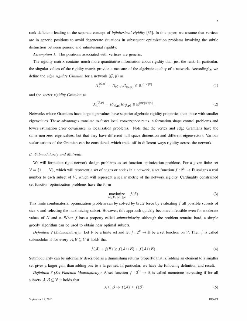
Example 1: Consider Fig. 1. Both networks depicted in Fig. 1 are constructed by the application of the Henneberg

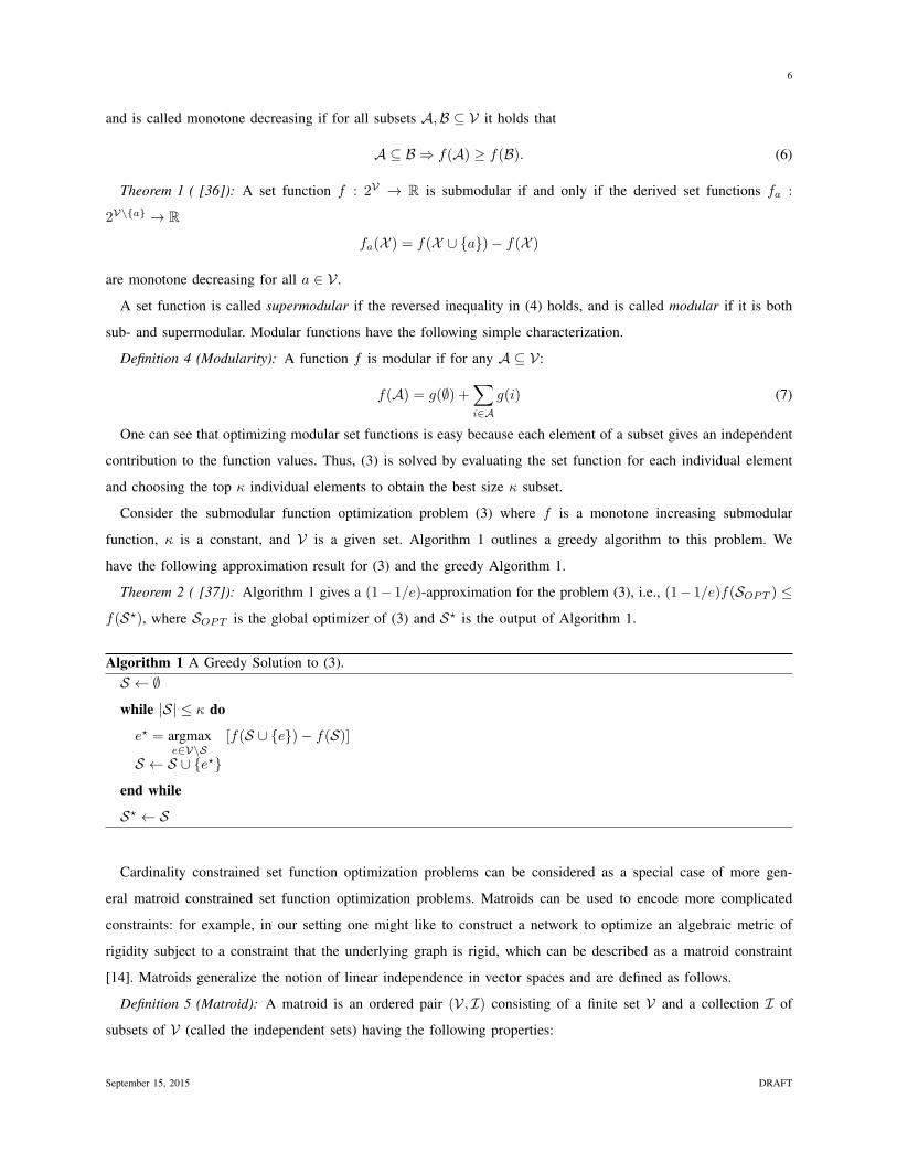
sequence and as a result are generically minimally rigid. Now, consider Fig. 2, where the networks have the same

underlying graph as those in Fig. 1 with the difference that nodes 1 and 4 are nearly collocated. In the new

configuration, the network depicted on the left exhibits weak algebraic rigidity properties: one can see that if node

4 is placed on top of node 1, node 5 can take infinitely many positions satisfying the edge length constraints

‖p1 − p5‖ = d15 and ‖p4 − p5‖ = d45. This corresponds to a rank deficiency in the rigidity Gramian. If the goal

was to localize the nodes given noisy distance measurements, the variance of the position estimate for node 5 would

approach infinity as the distance between nodes 1 and 4 goes to zero. The network on the right does not suffer

from this problem even if nodes 1 and 4 are collocated. In terms of algebraic rigidity, the graph structure on the

right is highly preferred given the positions in Fig. 2.

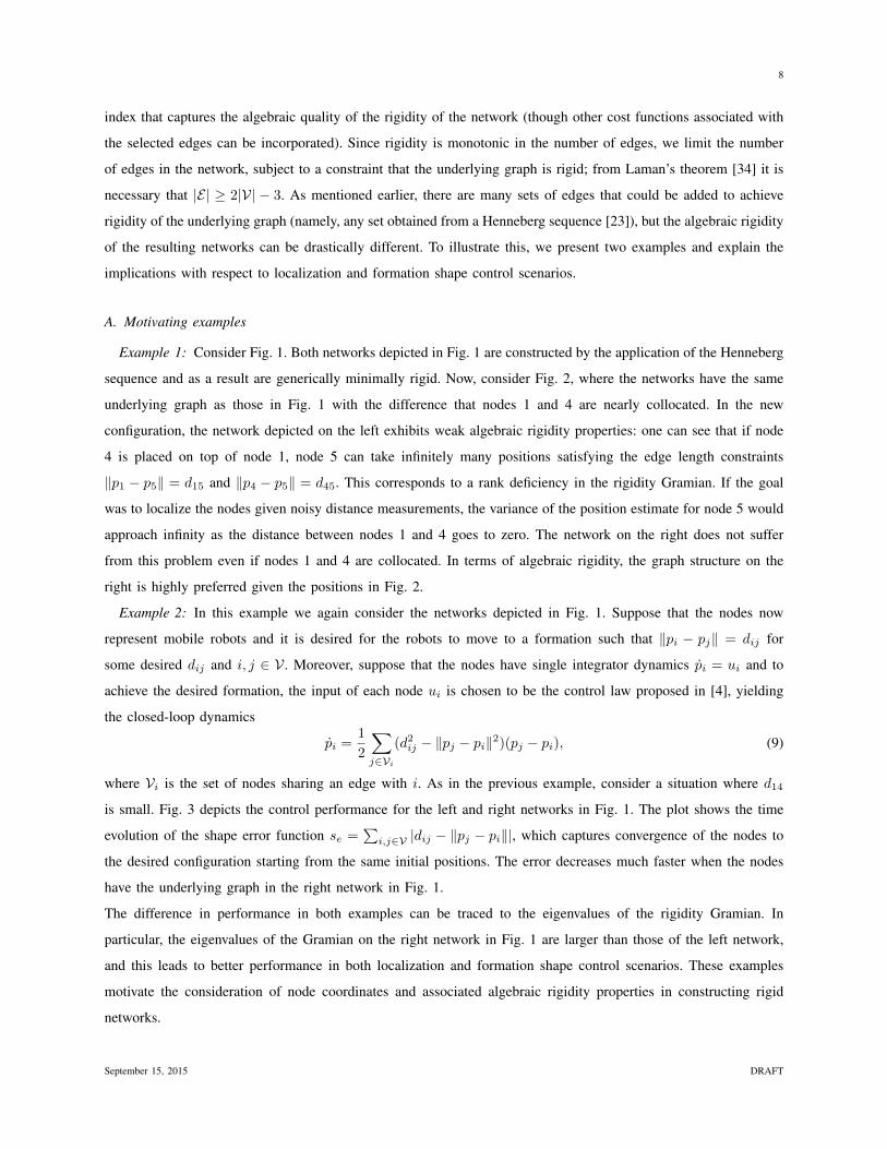
Example 2: In this example we again consider the networks depicted in Fig. 1. Suppose that the nodes now

represent mobile robots and it is desired for the robots to move to a formation such that ‖pi − pj‖ = dij for

some desired dij and i, j ∈ V . Moreover, suppose that the nodes have single integrator dynamics pi = ui and to

achieve the desired formation, the input of each node ui is chosen to be the control law proposed in [4], yielding

the closed-loop dynamics

pi =1

2

∑j∈Vi

(d2ij − ‖pj − pi‖2)(pj − pi), (9)

where Vi is the set of nodes sharing an edge with i. As in the previous example, consider a situation where d14

is small. Fig. 3 depicts the control performance for the left and right networks in Fig. 1. The plot shows the time

evolution of the shape error function se =∑i,j∈V |dij − ‖pj − pi‖|, which captures convergence of the nodes to

the desired configuration starting from the same initial positions. The error decreases much faster when the nodes

have the underlying graph in the right network in Fig. 1.

The difference in performance in both examples can be traced to the eigenvalues of the rigidity Gramian. In

particular, the eigenvalues of the Gramian on the right network in Fig. 1 are larger than those of the left network,

and this leads to better performance in both localization and formation shape control scenarios. These examples

motivate the consideration of node coordinates and associated algebraic rigidity properties in constructing rigid

networks.


9

1 3

5

4

21 3

5

4

2

Fig. 1. Two different networks obtained from the application of the Henneberg sequence. Hence, the underlying graphs are generically rigid.

1 3

5

1,4

21 3

5

1,4

2

5

Fig. 2. Although the underlying graphs are generically rigid, the relative node positions can lead to significantly different algebraic rigidity

properties. The network on the left ceases to be rigid when nodes 1 and 4 become collocated (and have very low algebraic rigidity when nearly

collocated). Thus, the network on the right is highly preferred for these particular relative positions.

B. Problem statement

The following statement formalizes the problem of interest.

Problem 1: Given a finite set of nodes V and a generic coordinate mapping p ∈ R2|V|, solve the following

0 10 20 30 40 50Time

0.0

0.1

0.2

0.3

0.4

0.5

0.6

Err

or

in Inte

r-node D

ista

nce

s

Left NetworkRight Network

Fig. 3. The performance of a formation shape control strategy for two different networks.


10

optimization problem

maximizeE

f(E)

subject to (G,p) is rigid

G = (V, E), |E| ≤ κ

(10)

where G is the underlying graph with vertex set V and the variable edge set E , p corresponds to the nodes

coordinates, f : 2V → R is a monotone increasing set function that quantifies the algebraic rigidity of the network,

and κ ≥ 2|V| − 3 is a given constant.

This problem is an NP-hard combinatorial optimization problem. However, we will show that several scalar functions

of the rigidity Gramian quantifying algebraic rigidity are modular or submodular set functions. The problem can be

split into two stages. In the first stage, a minimally rigid graph is constructed while optimizing an algebraic rigidity

metric, which can be cast as a matroid constrained submodular maximization problem. In the second stage, after

minimal rigidity has been achieved, an algebraic rigidity metric is further optimized while the remaining edges are

added, which can be cast as a cardinality constrained submodular maximization problem. As a consequence of the

modularity and submodularity properties, each stage comes with global optimality or near optimality guarantees

per Theorems 2 and 3 via simple greedy algorithms.

First, we rewrite the rigidity constraint of the network (G,p) in terms of the rank of the associated rigidity matrix

R(G,p). Thus (10) can be rewritten as

maximizeE

f(E)

subject to rank(R(G,p)) = 2|V| − 3

G = (V, E), |E| ≤ κ

(11)

The proposed solution to (11) consists of two stages. In the first stage, we consider a special case of (10), where

(G,p) is required to be minimally rigid, in which case |E| = 2|V| − 3:

maximizeE

f(E)

subject to rank(R(G,p)) = 2|V| − 3

G = (V, E), |E| = 2|V| − 3.

(12)

After a minimally rigid graph has beed constructed, the rank constraint is unnecessary. So in the second stage, the

remaining κ− (2|V| − 3) edges are added by solving

maximizeE

f(E)

subject to ES1,OPT ⊂ E

G = (V, E), |E| ≤ κ,

(13)

where ES1,OPT is the result of the algorithm for (12). In what follows, we elaborate on our proposed algorithms

for solving (12) and (13).


11

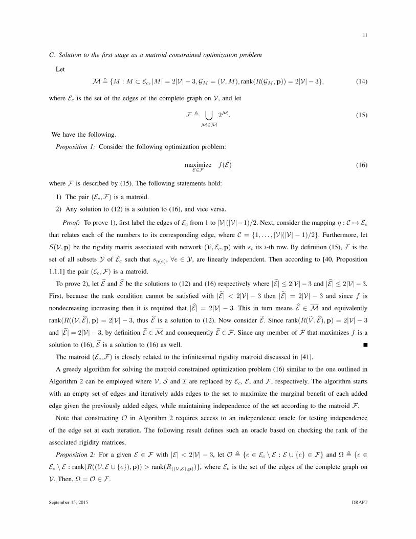
C. Solution to the first stage as a matroid constrained optimization problem

Let

M , M : M ⊂ Ec, |M | = 2|V| − 3,GM = (V,M), rank(R(GM ,p)) = 2|V| − 3, (14)

where Ec is the set of the edges of the complete graph on V , and let

F ,⋃M∈M

2M. (15)

We have the following.

Proposition 1: Consider the following optimization problem:

maximizeE∈F

f(E) (16)

where F is described by (15). The following statements hold:

1) The pair (Ec,F) is a matroid.

2) Any solution to (12) is a solution to (16), and vice versa.

Proof: To prove 1), first label the edges of Ec from 1 to |V|(|V|−1)/2. Next, consider the mapping η : C 7→ Ecthat relates each of the numbers to its corresponding edge, where C = 1, . . . , |V|(|V| − 1)/2. Furthermore, let

S(V,p) be the rigidity matrix associated with network (V, Ec,p) with si its i-th row. By definition (15), F is the

set of all subsets Y of Ec such that sη(e), ∀e ∈ Y , are linearly independent. Then according to [40, Proposition

1.1.1] the pair (Ec,F) is a matroid.

To prove 2), let E and E be the solutions to (12) and (16) respectively where |E | ≤ 2|V| − 3 and |E | ≤ 2|V| − 3.

First, because the rank condition cannot be satisfied with |E | < 2|V| − 3 then |E | = 2|V| − 3 and since f is

nondecreasing increasing then it is required that |E | = 2|V| − 3. This in turn means E ∈ M and equivalently

rank(R((V, E),p) = 2|V| − 3, thus E is a solution to (12). Now consider E . Since rank(R(V , E),p) = 2|V| − 3

and |E | = 2|V| − 3, by definition E ∈ M and consequently E ∈ F . Since any member of F that maximizes f is a

solution to (16), E is a solution to (16) as well.

The matroid (Ec,F) is closely related to the infinitesimal rigidity matroid discussed in [41].

A greedy algorithm for solving the matroid constrained optimization problem (16) similar to the one outlined in

Algorithm 2 can be employed where V , S and I are replaced by Ec, E , and F , respectively. The algorithm starts

with an empty set of edges and iteratively adds edges to the set to maximize the marginal benefit of each added

edge given the previously added edges, while maintaining independence of the set according to the matroid F .

Note that constructing O in Algorithm 2 requires access to an independence oracle for testing independence

of the edge set at each iteration. The following result defines such an oracle based on checking the rank of the

associated rigidity matrices.

Proposition 2: For a given E ∈ F with |E| < 2|V| − 3, let O , e ∈ Ec \ E : E ∪ e ∈ F and Ω , e ∈

Ec \ E : rank(R((V, E ∪ e),p)) > rank(R((V,E),p)), where Ec is the set of the edges of the complete graph on

V . Then, Ω = O ∈ F .


12

Proof: First, note that for any E ∈ F , |E| = rank(R((V,E),p)) by definition. Consequently, if for some

e ∈ Ec \ E , E ∪ e ∈ F , then rank(R((V, E ∪ e),p)) = |E|+ 1 > rank(R((V,E),p)). Thus, for any e ∈ O, also

e ∈ Ω. The proof for the reverse direction follows in a similar way.

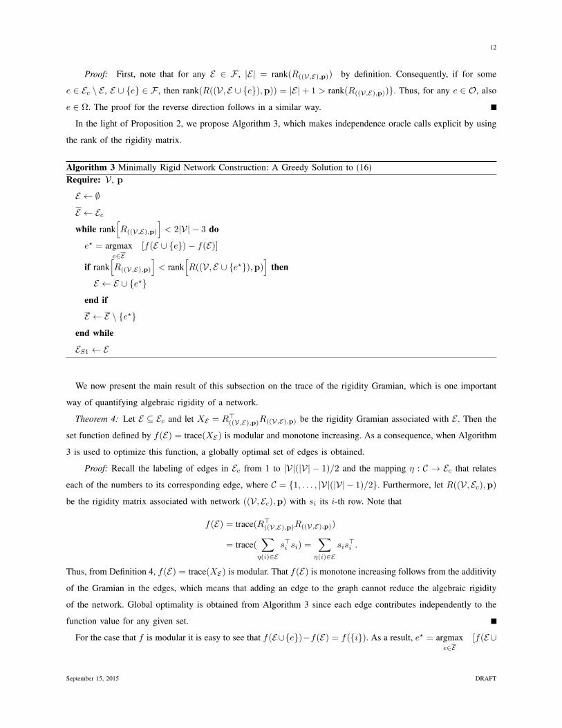
In the light of Proposition 2, we propose Algorithm 3, which makes independence oracle calls explicit by using

the rank of the rigidity matrix.

Algorithm 3 Minimally Rigid Network Construction: A Greedy Solution to (16)Require: V , p

E ← ∅

E ← Ecwhile rank

[R((V,E),p)

]< 2|V| − 3 do

e? = argmaxe∈E

[f(E ∪ e)− f(E)]

if rank[R((V,E),p)

]< rank

[R((V, E ∪ e?),p)

]then

E ← E ∪ e?

end if

E ← E \ e?

end while

ES1 ← E

We now present the main result of this subsection on the trace of the rigidity Gramian, which is one important

way of quantifying algebraic rigidity of a network.

Theorem 4: Let E ⊆ Ec and let XE = R>((V,E),p)R((V,E),p) be the rigidity Gramian associated with E . Then the

set function defined by f(E) = trace(XE) is modular and monotone increasing. As a consequence, when Algorithm

3 is used to optimize this function, a globally optimal set of edges is obtained.

Proof: Recall the labeling of edges in Ec from 1 to |V|(|V| − 1)/2 and the mapping η : C → Ec that relates

each of the numbers to its corresponding edge, where C = 1, . . . , |V|(|V| − 1)/2. Furthermore, let R((V, Ec),p)

be the rigidity matrix associated with network ((V, Ec),p) with si its i-th row. Note that

f(E) = trace(R>((V,E),p)R((V,E),p))

= trace(∑η(i)∈E

s>i si) =∑η(i)∈E

sis>i .

Thus, from Definition 4, f(E) = trace(XE) is modular. That f(E) is monotone increasing follows from the additivity

of the Gramian in the edges, which means that adding an edge to the graph cannot reduce the algebraic rigidity

of the network. Global optimality is obtained from Algorithm 3 since each edge contributes independently to the

function value for any given set.

For the case that f is modular it is easy to see that f(E∪e)−f(E) = f(i). As a result, e? = argmaxe∈E

[f(E∪


13

e) − f(E)] in Algorithm 3 can be replaced by e? = argmaxe∈E

f(i). This results in a more computationally

efficient algorithm since f is evaluated at most |Ec| times.

If f is submodular, the set ES1 obtained from Algorithm 3 satisfies the performance guarantee f(ES1,OPT )/2 ≤

f(ES1), where ES1,OPT is the global maximizer of f in the first stage problem (12) [37]. One can imagine alternative

spectral functions of the rigidity Gramian to optimize, such as trace of the pseudoinverse or the product of non-zero

eigenvalues. Since in Algorithm 3 the rigidity matrix changes rank at each iteration, it is not clear how to prove if

these or other functions are submodular. However, we will see in the next subsection that in the second stage we

can prove submodularity of other functions.

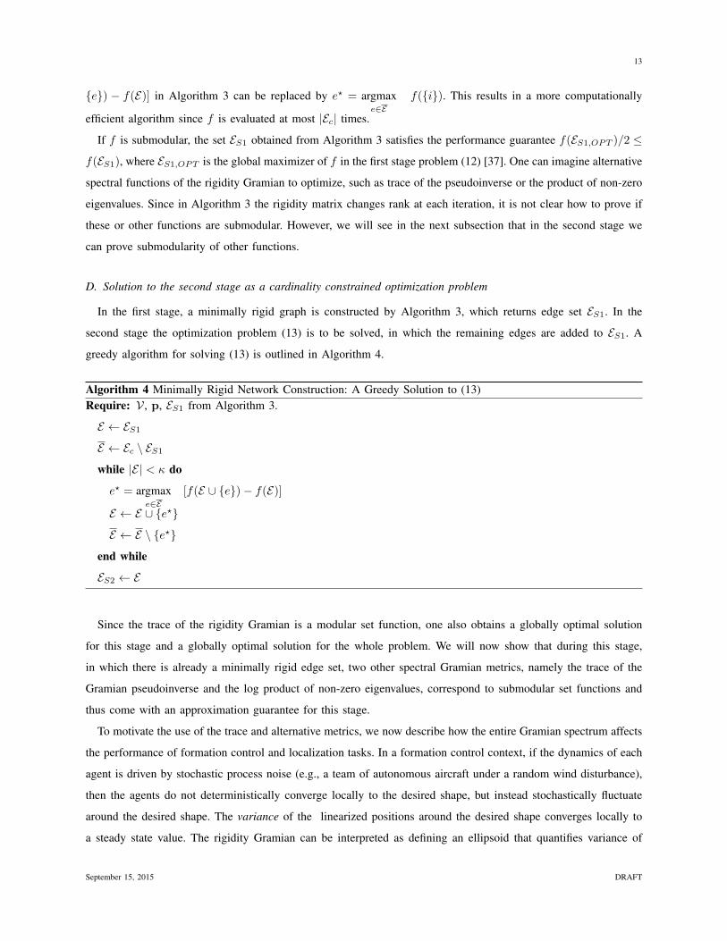
D. Solution to the second stage as a cardinality constrained optimization problem

In the first stage, a minimally rigid graph is constructed by Algorithm 3, which returns edge set ES1. In the

second stage the optimization problem (13) is to be solved, in which the remaining edges are added to ES1. A

greedy algorithm for solving (13) is outlined in Algorithm 4.

Algorithm 4 Minimally Rigid Network Construction: A Greedy Solution to (13)Require: V , p, ES1 from Algorithm 3.

E ← ES1E ← Ec \ ES1while |E| < κ do

e? = argmaxe∈E

[f(E ∪ e)− f(E)]

E ← E ∪ e?

E ← E \ e?

end while

ES2 ← E

Since the trace of the rigidity Gramian is a modular set function, one also obtains a globally optimal solution

for this stage and a globally optimal solution for the whole problem. We will now show that during this stage,

in which there is already a minimally rigid edge set, two other spectral Gramian metrics, namely the trace of the

Gramian pseudoinverse and the log product of non-zero eigenvalues, correspond to submodular set functions and

thus come with an approximation guarantee for this stage.

To motivate the use of the trace and alternative metrics, we now describe how the entire Gramian spectrum affects

the performance of formation control and localization tasks. In a formation control context, if the dynamics of each

agent is driven by stochastic process noise (e.g., a team of autonomous aircraft under a random wind disturbance),

then the agents do not deterministically converge locally to the desired shape, but instead stochastically fluctuate

around the desired shape. The variance of the linearized positions around the desired shape converges locally to

a steady state value. The rigidity Gramian can be interpreted as defining an ellipsoid that quantifies variance of


14

linearized relative position control errors, and all eigenvalues of the rigidity Gramian contribute to errors in various

directions. The trace of the Gramian pseudoinverse is then proportional to the average value of the error variance

in different directions, and the log product of non-zero eigenvalues of the Gramian is a volumetric quantification

of the steady state errors. In a localization setting, the rigidity Gramian and its pseudoinverse are closely related

to the Fisher Information Matrix and estimation error covariance associated with linearized position estimates,

discussed in more detail below. Similarly, the Gramian defines an uncertainty ellipsoid, and all eigenvalues of the

Gramian contribute to estimation errors in various directions; the trace is related to Fisher Information, the trace

of the pseudoinverse is proportional to average variance, and the eigenvalue product has volumetric and entropy

interpretations.

We have the following result.

Theorem 5: Let E ⊆ Ec and let XE = R>((V,E),p)R((V,E),p) be the rigidity Gramian associated with E . Moreover,

assume that there exists an edge set E? such that ((V, E?),p) is minimally rigid, i.e. rank((V, E?),p) = 2|V| − 3,

and E? ⊆ E . The following set functions are submodular and monotone increasing

1) f1(E) = −trace(X†E), where X†E denotes the Moore-Penrose pseudoinverse of XE .

2) f2(E) = log

(∏rank(XE)i=1 λi(XE)

)where λi(XE) is the i-th eigenvalue of XE and λ1(XE) ≥ · · · ≥ λn(XE).

As a consequence, when Algorithm 4 is used to optimize these functions, the approximation guarantees provided

by Theorems 2 and 3 are obtained.

Proof: We will use the characterization in Theorem 1 to prove the result. Similar to the preceding proof of

modularity for the trace metric, the key structure that can be exploited is the additivity of the rigidity Gramian with

respect to elements of E .

Trace of the inverse: Take an arbitrary e ∈ Ec and consider the derived set functions fe : 2Ec\e → R given by

fe(E) = −trace(X†E∪e) + trace(X†E)

= −trace((XE +Xe)†) + trace(X†E).

Take any E1 ⊆ E2 ⊆ Ec \ e. By the additivity property of the Gramian, it is clear that E1 ⊆ E2 ⇒ XE1 XE2 .

Now define X(t) = XE1 + t(XE2 −XE1) for t ∈ [0, 1]. Obviously, X(0) = XE1 and X(1) = XE2 . Now define

fe(X(t)) = −trace((X(t) +Xe)†) + trace(X(t)†).

Note that fe(X(0)) = fe(E1) and fe(X(1)) = fe(E2). We have

d

dtfe (X(t)) =

d

dt

[−trace((X(t) +Xe)

†) + trace(X(t)†)]

= trace[(X(t) +Xe)

†(XE2 −XE1)(X(t) +Xe)†]− trace

[X(t)†(XE2 −XE1)X(t)†

]= trace

[ ((X(t) +Xe)

†,2 −X(t)†,2)

(XE2 −XE1)

]≤ 0.

To obtain the second equality we used the matrix derivative formula ddt trace(X(t)†) = trace(X(t)† ddt (X(t))X(t)†)

which holds whenever X(t) has constant rank for all t, which we have here due to the assumption that there already

exists a set of edges that provides rigidity. To obtain the third equality we used the cyclic property of trace. Since


15

(X(t) +Xe)†,2 −X(t)†,2 0 and XE2 −XE1 0, the last inequality holds because the trace of the product of a

positive and negative semidefinite matrix is non-positive. Since

fe(X(1)) = fe(X(0)) +

∫ 1

0

d

dtfe(X(t))dt,

it follows that fe(X(1)) = fe(E2) ≤ fe(X(0)) = fe(E1). Thus, fe is monotone decreasing, and f1 is submodular

by Theorem 1.

Finally, it can be seen from additivity of the rigidity Gramian that f is monotone increasing, which just means

that adding an edge to the graph cannot decrease its rigidity.

Product of non-zero eigenvalues: The proof for the product of non-zero eigenvalues has the same structure.

Take any e ∈ Ec. Since rank(XE) = rank(XE∪e), from Lemma 1 in the appendix we know that there exists a P

such that

log

( rank(XE)∏i=1

λi(XE)

)= log det(XE)

andlog

(∏rank(XE∪e)

i=1 λi(XE∪e)

)= log

(∏rank(XE)i=1 λi(XE∪e)

)= log det(XE∪e)

where XE = XE + P and XE∪e = XE∪e + P . So, it is enough to show the submodularity of log det(XE).

Consider the derived set functions fe : 2Ec\e → R given by

fe(E) = log det XE∪e − log det XE

= log det(XE +Xe)− log det XE .

Take any E1 ⊆ E2 ⊆ Ec \ e, remember that XE1 XE2 , and define X(t) = (XE1 +P ) + t(

(XE2 +P )− (XE1 +

P ))

= (XE1 + P ) + t(XE2 −XE1) for t ∈ [0, 1] and

fe(X(t)) = log det(X(t) +Xe)− log det X(t).

Since we assumed that there exists a set of edges that provides rigidity and P is constant, X(t) has full rank for

all t, and it follows that

d

dtfe (X(t)) =

d

dt

[log det(X(t) +Xe)− log det X(t)

]= trace

[(X(t) +Xe)

−1(XE2 −XE1)]− trace

[X(t)−1(XE2 −XE1)

]= trace

[((X(t) +Xe)

−1 − X(t)−1)

(XE2 −XE1)

]≤ 0.

We used the matrix derivative formula ddt log det X(t) = trace[X(t)−1 ddtX(t)]. The remainder of the proof follows

the previous proof for trace of the inverse.

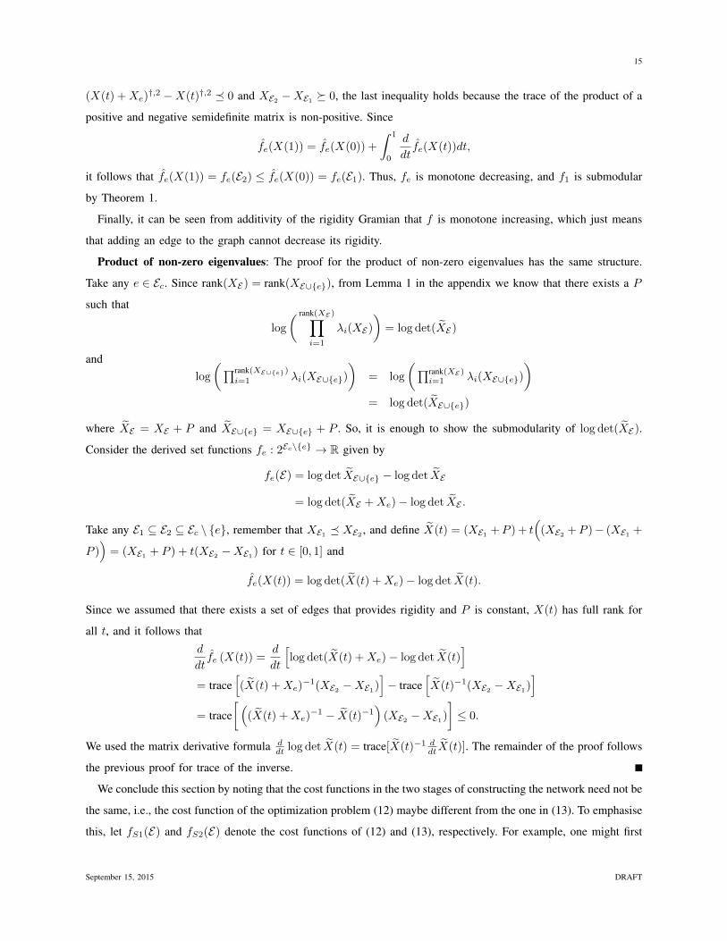
We conclude this section by noting that the cost functions in the two stages of constructing the network need not be

the same, i.e., the cost function of the optimization problem (12) maybe different from the one in (13). To emphasise

this, let fS1(E) and fS2(E) denote the cost functions of (12) and (13), respectively. For example, one might first


16

construct a minimally rigid via applying Algorithm 3 for the case where fS1(E) = trace(XE) and then add extra

edges to this minimally rigid network though the application of Algorithm 4 where fS2(E) =∏rank(XE)i=1 λi(XE),

where XE is the rigidity Gramian associated with E ⊂ Ec as defined earlier.

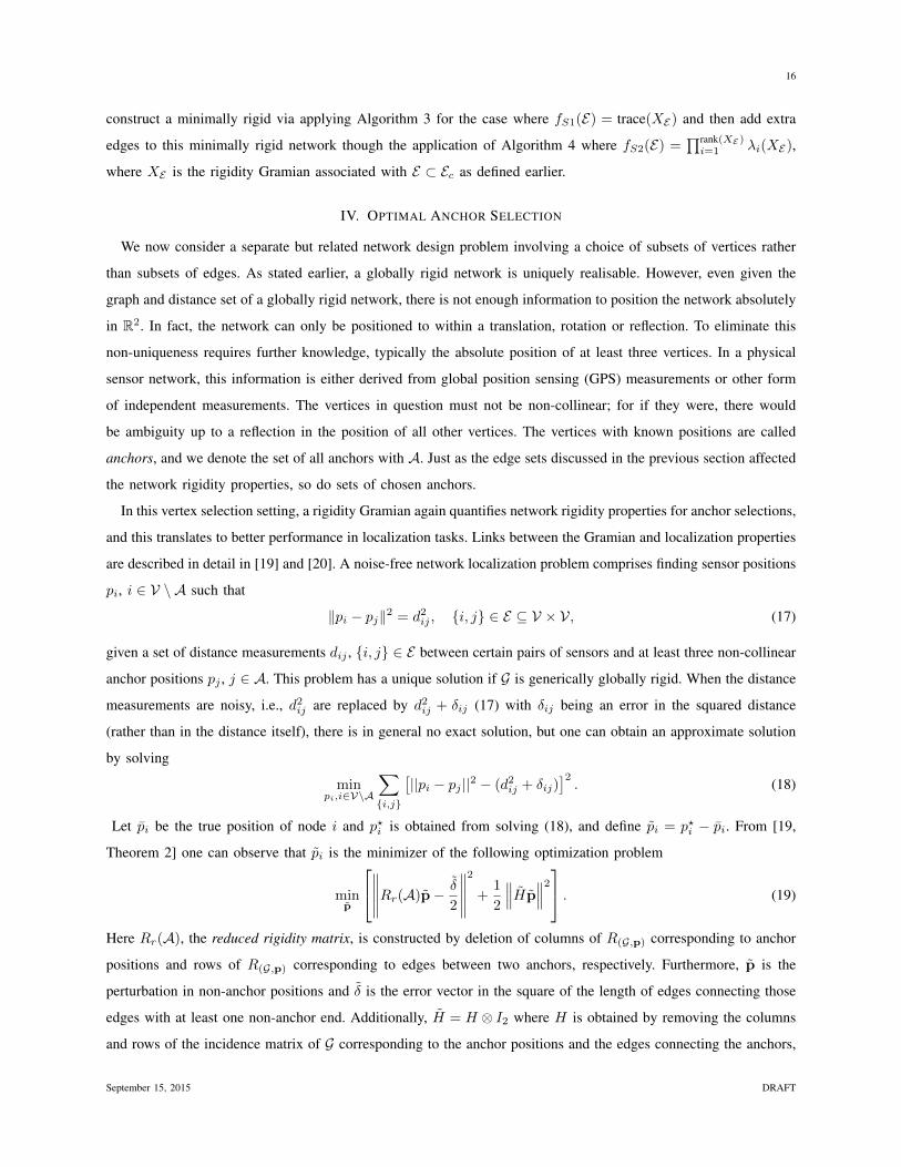
IV. OPTIMAL ANCHOR SELECTION

We now consider a separate but related network design problem involving a choice of subsets of vertices rather

than subsets of edges. As stated earlier, a globally rigid network is uniquely realisable. However, even given the

graph and distance set of a globally rigid network, there is not enough information to position the network absolutely

in R2. In fact, the network can only be positioned to within a translation, rotation or reflection. To eliminate this

non-uniqueness requires further knowledge, typically the absolute position of at least three vertices. In a physical

sensor network, this information is either derived from global position sensing (GPS) measurements or other form

of independent measurements. The vertices in question must not be non-collinear; for if they were, there would

be ambiguity up to a reflection in the position of all other vertices. The vertices with known positions are called

anchors, and we denote the set of all anchors with A. Just as the edge sets discussed in the previous section affected

the network rigidity properties, so do sets of chosen anchors.

In this vertex selection setting, a rigidity Gramian again quantifies network rigidity properties for anchor selections,

and this translates to better performance in localization tasks. Links between the Gramian and localization properties

are described in detail in [19] and [20]. A noise-free network localization problem comprises finding sensor positions

pi, i ∈ V \ A such that

‖pi − pj‖2 = d2ij , i, j ∈ E ⊆ V × V, (17)

given a set of distance measurements dij , i, j ∈ E between certain pairs of sensors and at least three non-collinear

anchor positions pj , j ∈ A. This problem has a unique solution if G is generically globally rigid. When the distance

measurements are noisy, i.e., d2ij are replaced by d2ij + δij (17) with δij being an error in the squared distance

(rather than in the distance itself), there is in general no exact solution, but one can obtain an approximate solution

by solving

minpi,i∈V\A

∑i,j

[||pi − pj ||2 − (d2ij + δij)

]2. (18)

Let pi be the true position of node i and p?i is obtained from solving (18), and define pi = p?i − pi. From [19,

Theorem 2] one can observe that pi is the minimizer of the following optimization problem

minp

∥∥∥∥∥Rr(A)p− δ

2

∥∥∥∥∥2

+1

2

∥∥∥Hp∥∥∥2 . (19)

Here Rr(A), the reduced rigidity matrix, is constructed by deletion of columns of R(G,p) corresponding to anchor

positions and rows of R(G,p) corresponding to edges between two anchors, respectively. Furthermore, p is the

perturbation in non-anchor positions and δ is the error vector in the square of the length of edges connecting those

edges with at least one non-anchor end. Additionally, H = H ⊗ I2 where H is obtained by removing the columns

and rows of the incidence matrix of G corresponding to the anchor positions and the edges connecting the anchors,


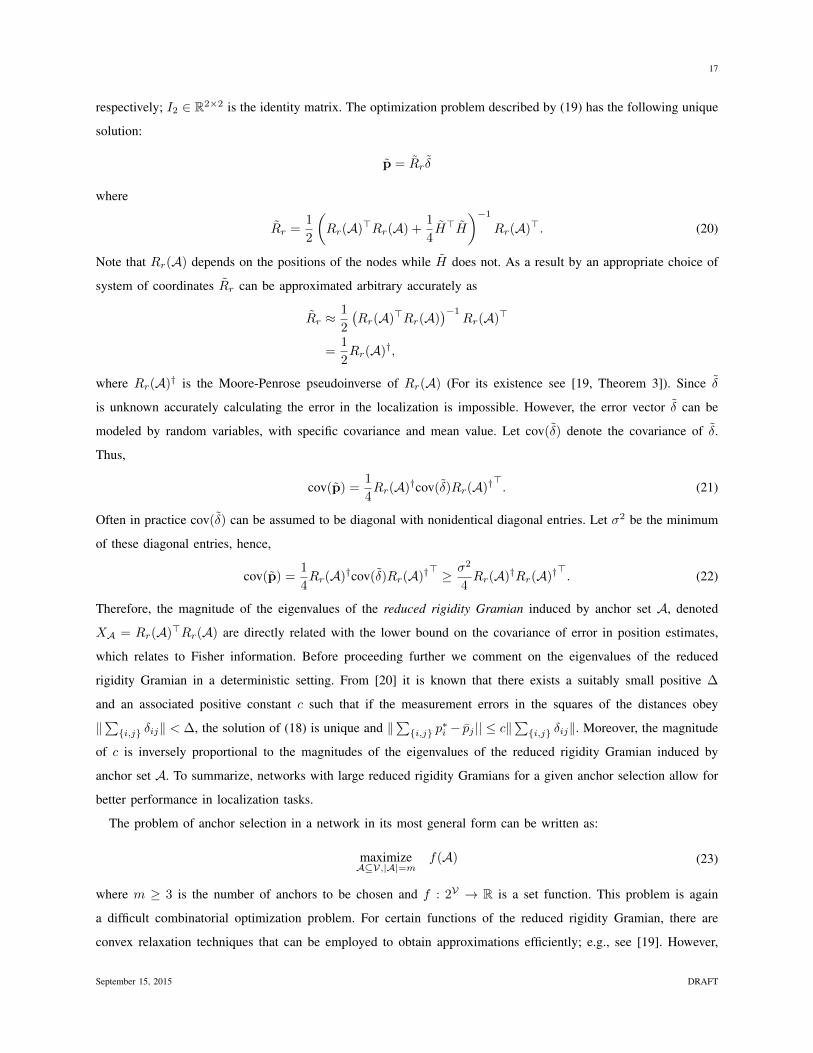
17

respectively; I2 ∈ R2×2 is the identity matrix. The optimization problem described by (19) has the following unique

solution:

p = Rr δ

where

Rr =1

2

(Rr(A)>Rr(A) +

1

4H>H

)−1Rr(A)>. (20)

Note that Rr(A) depends on the positions of the nodes while H does not. As a result by an appropriate choice of

system of coordinates Rr can be approximated arbitrary accurately as

Rr ≈1

2

(Rr(A)>Rr(A)

)−1Rr(A)>

=1

2Rr(A)†,

where Rr(A)† is the Moore-Penrose pseudoinverse of Rr(A) (For its existence see [19, Theorem 3]). Since δ

is unknown accurately calculating the error in the localization is impossible. However, the error vector δ can be

modeled by random variables, with specific covariance and mean value. Let cov(δ) denote the covariance of δ.

Thus,

cov(p) =1

4Rr(A)†cov(δ)Rr(A)†

>. (21)

Often in practice cov(δ) can be assumed to be diagonal with nonidentical diagonal entries. Let σ2 be the minimum

of these diagonal entries, hence,

cov(p) =1

4Rr(A)†cov(δ)Rr(A)†

> ≥ σ2

4Rr(A)†Rr(A)†

>. (22)

Therefore, the magnitude of the eigenvalues of the reduced rigidity Gramian induced by anchor set A, denoted

XA = Rr(A)>Rr(A) are directly related with the lower bound on the covariance of error in position estimates,

which relates to Fisher information. Before proceeding further we comment on the eigenvalues of the reduced

rigidity Gramian in a deterministic setting. From [20] it is known that there exists a suitably small positive ∆

and an associated positive constant c such that if the measurement errors in the squares of the distances obey

‖∑i,j δij‖ < ∆, the solution of (18) is unique and ‖

∑i,j p

∗i − pj || ≤ c‖

∑i,j δij‖. Moreover, the magnitude

of c is inversely proportional to the magnitudes of the eigenvalues of the reduced rigidity Gramian induced by

anchor set A. To summarize, networks with large reduced rigidity Gramians for a given anchor selection allow for

better performance in localization tasks.

The problem of anchor selection in a network in its most general form can be written as:

maximizeA⊆V,|A|=m

f(A) (23)

where m ≥ 3 is the number of anchors to be chosen and f : 2V → R is a set function. This problem is again

a difficult combinatorial optimization problem. For certain functions of the reduced rigidity Gramian, there are

convex relaxation techniques that can be employed to obtain approximations efficiently; e.g., see [19]. However,


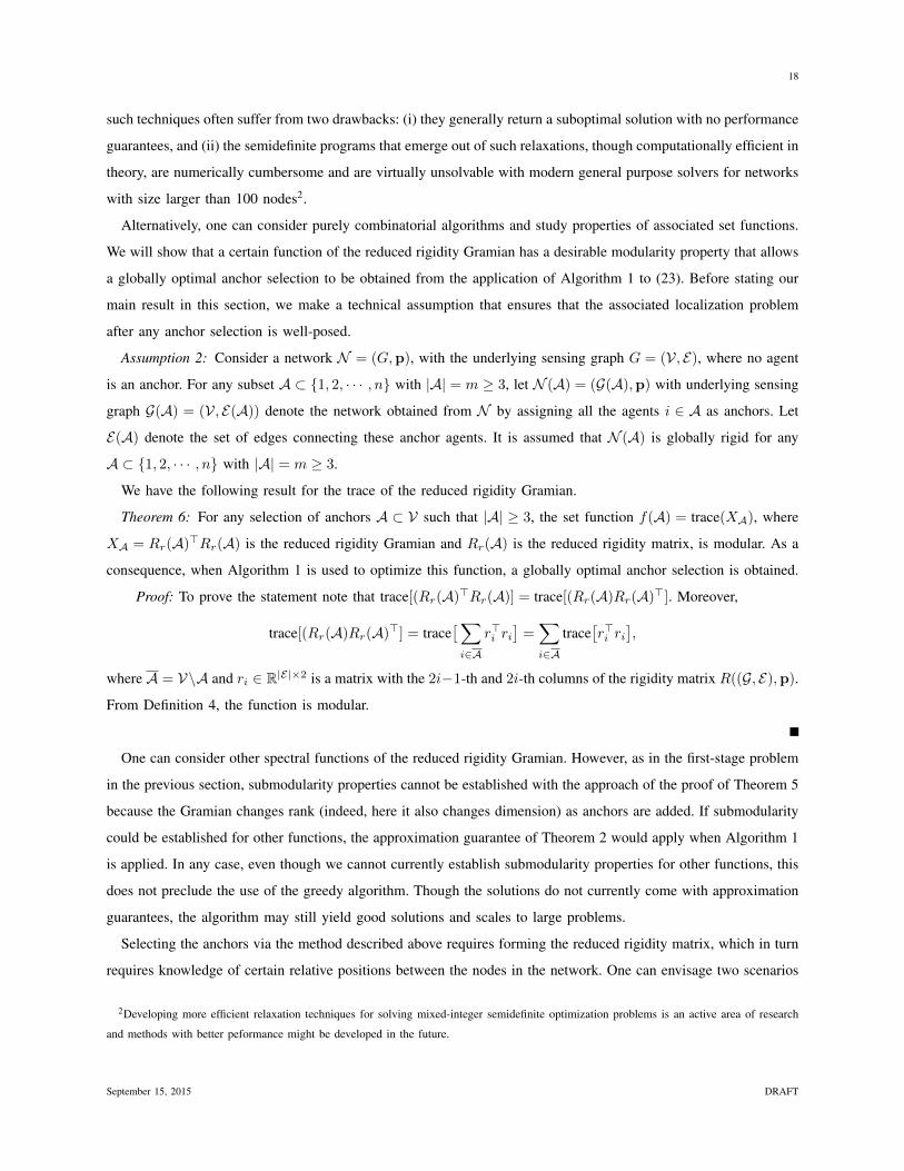
18

such techniques often suffer from two drawbacks: (i) they generally return a suboptimal solution with no performance

guarantees, and (ii) the semidefinite programs that emerge out of such relaxations, though computationally efficient in

theory, are numerically cumbersome and are virtually unsolvable with modern general purpose solvers for networks

with size larger than 100 nodes2.

Alternatively, one can consider purely combinatorial algorithms and study properties of associated set functions.

We will show that a certain function of the reduced rigidity Gramian has a desirable modularity property that allows

a globally optimal anchor selection to be obtained from the application of Algorithm 1 to (23). Before stating our

main result in this section, we make a technical assumption that ensures that the associated localization problem

after any anchor selection is well-posed.

Assumption 2: Consider a network N = (G,p), with the underlying sensing graph G = (V, E), where no agent

is an anchor. For any subset A ⊂ 1, 2, · · · , n with |A| = m ≥ 3, let N (A) = (G(A),p) with underlying sensing

graph G(A) = (V, E(A)) denote the network obtained from N by assigning all the agents i ∈ A as anchors. Let

E(A) denote the set of edges connecting these anchor agents. It is assumed that N (A) is globally rigid for any

A ⊂ 1, 2, · · · , n with |A| = m ≥ 3.

We have the following result for the trace of the reduced rigidity Gramian.

Theorem 6: For any selection of anchors A ⊂ V such that |A| ≥ 3, the set function f(A) = trace(XA), where

XA = Rr(A)>Rr(A) is the reduced rigidity Gramian and Rr(A) is the reduced rigidity matrix, is modular. As a

consequence, when Algorithm 1 is used to optimize this function, a globally optimal anchor selection is obtained.

Proof: To prove the statement note that trace[(Rr(A)>Rr(A)] = trace[(Rr(A)Rr(A)>]. Moreover,

trace[(Rr(A)Rr(A)>] = trace[∑i∈A

r>i ri]

=∑i∈A

trace[r>i ri

],

where A = V\A and ri ∈ R|E|×2 is a matrix with the 2i−1-th and 2i-th columns of the rigidity matrix R((G, E),p).

From Definition 4, the function is modular.

One can consider other spectral functions of the reduced rigidity Gramian. However, as in the first-stage problem

in the previous section, submodularity properties cannot be established with the approach of the proof of Theorem 5

because the Gramian changes rank (indeed, here it also changes dimension) as anchors are added. If submodularity

could be established for other functions, the approximation guarantee of Theorem 2 would apply when Algorithm 1

is applied. In any case, even though we cannot currently establish submodularity properties for other functions, this

does not preclude the use of the greedy algorithm. Though the solutions do not currently come with approximation

guarantees, the algorithm may still yield good solutions and scales to large problems.

Selecting the anchors via the method described above requires forming the reduced rigidity matrix, which in turn

requires knowledge of certain relative positions between the nodes in the network. One can envisage two scenarios

2Developing more efficient relaxation techniques for solving mixed-integer semidefinite optimization problems is an active area of research

and methods with better peformance might be developed in the future.


19

in which the method could be used. First, suppose that multiple nodes in a sensor network have GPS receivers, and

to conserve energy it is desired that only a few receivers should be turned on for localization purposes. Initially,

a random subset of them may activate their GPS receivers so that a coarse localization can be done. Using the

information obtained from this initial optimization step, a rigidity matrix can be constructed, which consequently

makes selecting which nodes to turn on their GPS receivers, i.e., be selected as an anchor, in order to obtain a

better localization accuracy possible. Second, suppose that relative position information in the absence of a global

coordinate frame is available, however, finding the positions in a global coordinate frame requires fixing the position

of a subset of nodes, i.e., selecting some of them as anchors. This is particularly important when the nodes are

moving while maintaining their relative positions from each other.

V. NUMERICAL EXAMPLES

In this section, initially, we study the performance of the algorithms introduced in Section III.

In the first scenario, we compare the performance of Algorithms 3 and 4 with a semidefinite programming (SDP)

relaxation of (11) given below:

maximizeti

f(∑|V|(2|V|−1)/2i=1 tis

>i si)

subject to ti ∈ [0, 1],∑|V|(2|V|−1)/2i=1 ti = κ,

i = 1, . . . , |V|(2|V| − 1)/2,

B>(∑|V|(2|V|−1)/2

i=1 tis>i si

)B γI.

(24)

where si its i-th row of ((V, Ec),p) — the rigidity matrix associated with network , — B is a 2|V| × 2|V| − 3

matrix whose columns are orthogonal to the vectors in the null space of the rigidity Gramian of a rigid network—

i.e., they are orthogonal to [1, 0, 1, 0 . . . ]>, [0, 1, 0, 1, . . . ]>, and [y1,−x1, y2,−x2, . . . ]>, — and γ 1 is a small

positive constant. Consequently, the resulting network from solving (24) is obtained from selecting edges η(j)

(η : 1, . . . , |V|(|V| − 1)/2 → Ec relates each index j to its corresponding edge) where the corresponding t?j

obtained from (24) is among the κ-largest values of t?i , i = 1, . . . , |V|(2|V| − 1)/2. However, the network obtained

from solving (24) is not guaranteed to be rigid.

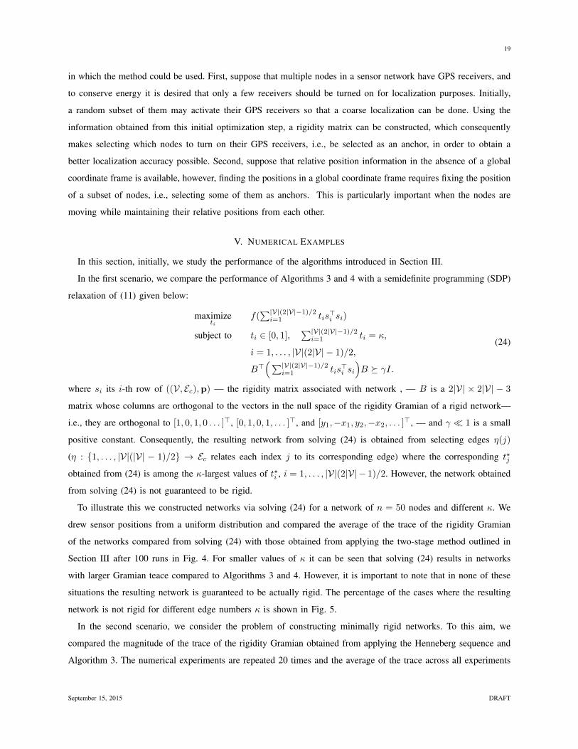
To illustrate this we constructed networks via solving (24) for a network of n = 50 nodes and different κ. We

drew sensor positions from a uniform distribution and compared the average of the trace of the rigidity Gramian

of the networks compared from solving (24) with those obtained from applying the two-stage method outlined in

Section III after 100 runs in Fig. 4. For smaller values of κ it can be seen that solving (24) results in networks

with larger Gramian teace compared to Algorithms 3 and 4. However, it is important to note that in none of these

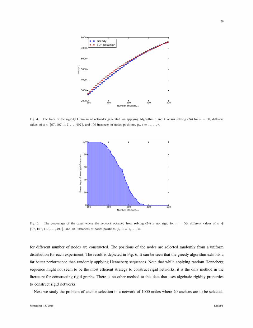
situations the resulting network is guaranteed to be actually rigid. The percentage of the cases where the resulting

network is not rigid for different edge numbers κ is shown in Fig. 5.

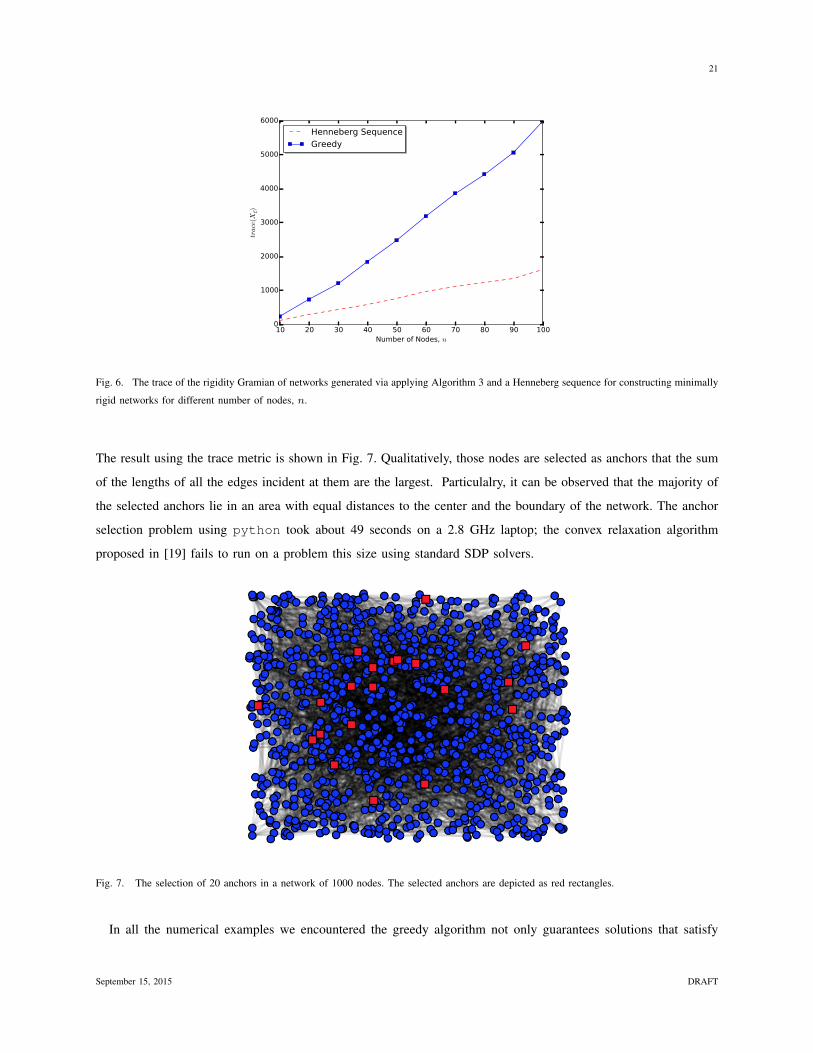
In the second scenario, we consider the problem of constructing minimally rigid networks. To this aim, we

compared the magnitude of the trace of the rigidity Gramian obtained from applying the Henneberg sequence and

Algorithm 3. The numerical experiments are repeated 20 times and the average of the trace across all experiments


20

100 200 300 400 500Number of Edges,

2000

3000

4000

5000

6000

7000

8000

trace

(XE)

GreedySDP Relaxtion

Fig. 4. The trace of the rigidity Gramian of networks generated via applying Algorithm 3 and 4 versus solving (24) for n = 50, different

values of κ ∈ 97, 107, 117, . . . , 497, and 100 instances of nodes positions, pi, i = 1, . . . , n.

100 200 300 400 500Number of Edges,

0

20

40

60

80

100

Perc

enta

ge o

f N

on-r

igid

Outc

om

es

Fig. 5. The percentage of the cases where the network obtained from solving (24) is not rigid for n = 50, different values of κ ∈97, 107, 117, . . . , 497, and 100 instances of nodes positions, pi, i = 1, . . . , n.

for different number of nodes are constructed. The positions of the nodes are selected randomly from a uniform

distribution for each experiment. The result is depicted in Fig. 6. It can be seen that the greedy algorithm exhibits a

far better performance than randomly applying Henneberg sequences. Note that while applying random Henneberg

sequence might not seem to be the most efficient strategy to construct rigid networks, it is the only method in the

literature for constructing rigid graphs. There is no other method to this date that uses algebraic rigidity properties

to construct rigid networks.

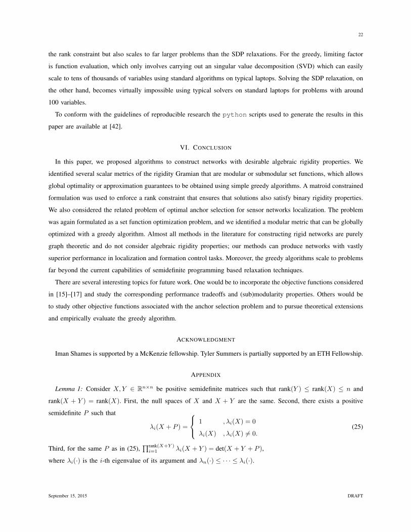
Next we study the problem of anchor selection in a network of 1000 nodes where 20 anchors are to be selected.


21

10 20 30 40 50 60 70 80 90 100Number of Nodes, n

0

1000

2000

3000

4000

5000

6000

trace

(XE)

Henneberg SequenceGreedy

Fig. 6. The trace of the rigidity Gramian of networks generated via applying Algorithm 3 and a Henneberg sequence for constructing minimally

rigid networks for different number of nodes, n.

The result using the trace metric is shown in Fig. 7. Qualitatively, those nodes are selected as anchors that the sum

of the lengths of all the edges incident at them are the largest. Particulalry, it can be observed that the majority of

the selected anchors lie in an area with equal distances to the center and the boundary of the network. The anchor

selection problem using python took about 49 seconds on a 2.8 GHz laptop; the convex relaxation algorithm

proposed in [19] fails to run on a problem this size using standard SDP solvers.

Fig. 7. The selection of 20 anchors in a network of 1000 nodes. The selected anchors are depicted as red rectangles.

In all the numerical examples we encountered the greedy algorithm not only guarantees solutions that satisfy


22

the rank constraint but also scales to far larger problems than the SDP relaxations. For the greedy, limiting factor

is function evaluation, which only involves carrying out an singular value decomposition (SVD) which can easily

scale to tens of thousands of variables using standard algorithms on typical laptops. Solving the SDP relaxation, on

the other hand, becomes virtually impossible using typical solvers on standard laptops for problems with around

100 variables.

To conform with the guidelines of reproducible research the python scripts used to generate the results in this

paper are available at [42].

VI. CONCLUSION

In this paper, we proposed algorithms to construct networks with desirable algebraic rigidity properties. We

identified several scalar metrics of the rigidity Gramian that are modular or submodular set functions, which allows

global optimality or approximation guarantees to be obtained using simple greedy algorithms. A matroid constrained

formulation was used to enforce a rank constraint that ensures that solutions also satisfy binary rigidity properties.

We also considered the related problem of optimal anchor selection for sensor networks localization. The problem

was again formulated as a set function optimization problem, and we identified a modular metric that can be globally

optimized with a greedy algorithm. Almost all methods in the literature for constructing rigid networks are purely

graph theoretic and do not consider algebraic rigidity properties; our methods can produce networks with vastly

superior performance in localization and formation control tasks. Moreover, the greedy algorithms scale to problems

far beyond the current capabilities of semidefinite programming based relaxation techniques.

There are several interesting topics for future work. One would be to incorporate the objective functions considered

in [15]–[17] and study the corresponding performance tradeoffs and (sub)modularity properties. Others would be

to study other objective functions associated with the anchor selection problem and to pursue theoretical extensions

and empirically evaluate the greedy algorithm.

ACKNOWLEDGMENT

Iman Shames is supported by a McKenzie fellowship. Tyler Summers is partially supported by an ETH Fellowship.

APPENDIX

Lemma 1: Consider X,Y ∈ Rn×n be positive semidefinite matrices such that rank(Y ) ≤ rank(X) ≤ n and

rank(X + Y ) = rank(X). First, the null spaces of X and X + Y are the same. Second, there exists a positive

semidefinite P such that

λi(X + P ) =

1 , λi(X) = 0

λi(X) , λi(X) 6= 0.(25)

Third, for the same P as in (25),∏rank(X+Y )i=1 λi(X + Y ) = det(X + Y + P ),

where λi(·) is the i-th eigenvalue of its argument and λn(·) ≤ · · · ≤ λi(·).


23

Proof: Let rank(X) = ρ and ui be the unit length eigenvectors of X associated with λi(X) such that u>i uj = 0

for i 6= j. For any j ∈ n−ρ+1, . . . , n, It follows that u>j (X+Y )uj = u>Y u. To obtain a contradiction assume

there is a j ∈ n− ρ+ 1, . . . , n such that u>j Y uj 6= 0. Thus the dimension of the null space of X +Y is at most

n− ρ− 1, which is equivalent to rank(X +Y ) = ρ+ 1 which is a contradiction. Hence, the spaces spanned by the

eigenvalues of X and X + Y are the same.

Second, because X is symmetric it can be diagonalised. Let X = UΛ(X)U>, where U>U = I , Λ(X) =

diag(λ1(X), . . . , λn(X)), and U =[u1 . . . un

]. Define P = UΛPU

> where ΛP has zero entries except the

ii-th diagonal entry of 1 if λi(X) = 0. Such a P satisfies (25) and P =∑ni=n−ρ+1 uiu

>i .

Third, X + Y = UΛ(X + Y )U>

, where U>U = I , Λ(X + Y ) = diag(λ1(X + Y ), . . . , λn(X + Y )), and

U =[u1 . . . un

]with ui being the i-th eigenvector of X + Y associated with λi(X + Y ). Similar to above

there exists a P =∑ni=n−ρ+1 uiu

>i such that

λi(X + Y + P ) =

1 , λi(X + Y ) = 0

λi(X + Y ) , λi(X + Y ) 6= 0.(26)

Hence, X + Y + P is nonsingular and∏rank(X+Y )i=1 λi(X + Y ) = det(X + Y + P ). Moreover, in light of the first

statement, ui = ui, i = n− ρ+ 1, . . . , n. Thus P = P and∏rank(X+Y )i=1 λi(X + Y ) = det(X + Y + P ).

REFERENCES

[1] R. Olfati-Saber and R. M. Murray, “Graph rigidity and distributed formation stabilization of multi-vehicle systems,” in Proceedings of the

41st IEEE Conference on Decision and Control, vol. 3. IEEE, 2002, pp. 2965–2971.

[2] B. D. Anderson, C. Yu, B. Fidan, and J. M. Hendrickx, “Rigid graph control architectures for autonomous formations,” IEEE Control

Systems Magazine, vol. 28, no. 6, pp. 48–63, 2008.

[3] C. Yu, J. M. Hendrickx, B. Fidan, B. Anderson, and V. D. Blondel, “Three and higher dimensional autonomous formations: Rigidity,

persistence and structural persistence,” Automatica, vol. 43, no. 3, pp. 387–402, 2007.

[4] L. Krick, M. E. Broucke, and B. A. Francis, “Stabilisation of infinitesimally rigid formations of multi-robot networks,” International

Journal of Control, vol. 82, no. 3, pp. 423–439, 2009.

[5] C. Yu, B. D. Anderson, S. Dasgupta, and B. Fidan, “Control of minimally persistent formations in the plane,” SIAM Journal on Control

and Optimization, vol. 48, no. 1, pp. 206–233, 2009.

[6] T. H. Summers, C. Yu, S. Dasgupta, and B. D. Anderson, “Control of minimally persistent leader-remote-follower and coleader formations

in the plane,” Automatic Control, IEEE Transactions on, vol. 56, no. 12, pp. 2778–2792, 2011.

[7] T. Eren, O. Goldenberg, W. Whiteley, Y. R. Yang, A. S. Morse, B. D. Anderson, and P. N. Belhumeur, “Rigidity, computation,

and randomization in network localization,” in INFOCOM 2004. Twenty-third AnnualJoint Conference of the IEEE Computer and

Communications Societies, vol. 4. IEEE, 2004, pp. 2673–2684.

[8] J. Aspnes, T. Eren, D. K. Goldenberg, A. S. Morse, W. Whiteley, Y. R. Yang, B. D. Anderson, and P. N. Belhumeur, “A theory of network

localization,” Mobile Computing, IEEE Transactions on, vol. 5, no. 12, pp. 1663–1678, 2006.

[9] D. Moore, J. Leonard, D. Rus, and S. Teller, “Robust distributed network localization with noisy range measurements,” in Proceedings of

the 2nd international conference on Embedded networked sensor systems. ACM, 2004, pp. 50–61.

[10] G. Mao, B. Fidan, and B. Anderson, “Wireless sensor network localization techniques,” Computer networks, vol. 51, no. 10, pp. 2529–2553,

2007.

[11] A. M.-C. So and Y. Ye, “Theory of semidefinite programming for sensor network localization,” Mathematical Programming, vol. 109, no.

2-3, pp. 367–384, 2007.

[12] B. Hendrickson, “Conditions for unique graph realizations,” SIAM Journal on Computing, vol. 21, no. 1, pp. 65–84, 1992.


24

[13] R. Connelly, “Generic global rigidity,” Discrete & Computational Geometry, vol. 33, no. 4, pp. 549–563, 2005.

[14] B. Jackson and T. Jordan, “Connected rigidity matroids and unique realizations of graphs,” Journal of Combinatorial Theory, Series B,

vol. 94, no. 1, pp. 1–29, 2005.

[15] R. Ren, Y.-Y. Zhang, X.-Y. Luo, and S.-B. Li, “Automatic generation of optimally rigid formations using decentralized methods,”

International Journal of Automation and Computing, vol. 7, no. 4, pp. 557–564, 2010.

[16] D. Zelazo and F. Allgower, “Growing optimally rigid formations,” in American Control Conference. IEEE, 2012, pp. 3901–3906.

[17] A. Priolo, R. Williams, A. Gasparri, and G. Sukhatme, “Decentralized algorithms for optimally rigid network constructions,” in IEEE

International Conference on Robotics and Automation. IEEE, 2014, pp. 5010–5015.

[18] A. Gasparri, R. Williams, A. Priolo, and R. Sukhatme, “Decentralized and parallel constructions for optimally rigid graphs in R2,” IEEE

Transactions on Mobile Computing, vol. 99, no. 1, pp. 1–1, 2015.

[19] I. Shames, B. Fidan, and B. Anderson, “Minimization of the effect of noisy measurements on localization of multi-agent autonomous

formations,” Automatica, vol. 45, no. 4, pp. 1058–1065, 2009.

[20] B. D. Anderson, I. Shames, G. Mao, and B. Fidan, “Formal theory of noisy sensor network localization,” SIAM Journal on Discrete

Mathematics, vol. 24, no. 2, pp. 684–698, 2010.

[21] D. Zelazo, A. Franchi, H. H. Bulthoff, and P. R. Giordano, “Decentralized rigidity maintenance control with range-only measurements for

multi-robot systems,” International Journal of Robotics Research, vol. 34, no. 1, pp. 105–128, 2015.

[22] L. Henneberg, Die graphische Statik der starren Systeme. BG Teubner, 1911, vol. 31.

[23] T.-S. Tay and W. Whiteley, “Generating isostatic frameworks,” Structural Topology, no. 11, 1985.

[24] P. Biswas, T.-C. Liang, K.-C. Toh, Y. Ye, and T.-C. Wang, “Semidefinite programming approaches for sensor network localization with

noisy distance measurements,” Automation Science and Engineering, IEEE Transactions on, vol. 3, no. 4, pp. 360–371, 2006.

[25] K. Langendoen and N. Reijers, “Distributed localization in wireless sensor networks: a quantitative comparison,” Computer Networks,

vol. 43, no. 4, pp. 499–518, 2003.

[26] S. P. Chepuri, G. Leus et al., “Sparsity-exploiting anchor placement for localization in sensor networks,” in Signal Processing Conference

(EUSIPCO), 2013 Proceedings of the 21st European. IEEE, 2013, pp. 1–5.

[27] J. N. Ash and R. L. Moses, “On optimal anchor node placement in sensor localization by optimization of subspace principal angles,” in

Acoustics, Speech and Signal Processing, 2008. ICASSP 2008. IEEE International Conference on. IEEE, 2008, pp. 2289–2292.

[28] N. Salman, H. K. Maheshwari, A. H. Kemp, and M. Ghogho, “Effects of anchor placement on mean-crb for localization,” in Ad Hoc

Networking Workshop (Med-Hoc-Net), 2011 The 10th IFIP Annual Mediterranean. IEEE, 2011, pp. 115–118.

[29] T. H. Summers and J. Lygeros, “Optimal sensor and actuator placement in complex dynamical networks,” in to appear at the IFAC World

Congress, 2014.

[30] F. L. Cortesi, T. H. Summers, and J. Lygeros, “Submodularity of energy related controllability metrics,” arXiv preprint arXiv:1403.6351,

2014.

[31] T. H. Summers, F. L. Cortesi, and J. Lygeros, “On submodularity and controllability in complex dynamical networks,” arXiv preprint

arXiv:1404.7665, 2014.

[32] T. Summers, I. Shames, J. Lygeros, and F. Dorfler, “Topology design for optimal network coherence,” in European Control Conference,

2015.

[33] A. Clark, L. Bushnell, and R. Poovendran, “A supermodular optimization framework for leader selection under link noise in linear multi-

agent systems,” IEEE Transactions on Automatic Control, vol. 59, no. 2, pp. 283–296, 2014.

[34] G. Laman, “On graphs and rigidity of plane skeletal structures,” Journal of Engineering mathematics, vol. 4, no. 4, pp. 331–340, 1970.

[35] L. Asimow and B. Roth, “The rigidity of graphs, ii,” Journal of Mathematical Analysis and Applications, vol. 68, no. 1, pp. 171–190,

1979.

[36] L. Lovasz, “Submodular functions and convexity,” in Mathematical Programming The State of the Art. Springer, 1983, pp. 235–257.

[37] G. L. Nemhauser, L. A. Wolsey, and M. L. Fisher, “An analysis of approximations for maximizing submodular set functions–i,” Mathematical

Programming, vol. 14, no. 1, pp. 265–294, 1978.

[38] M. L. Fisher, G. L. Nemhauser, and L. A. Wolsey, “An analysis of approximations for maximizing submodular set functions–ii,” Polyhedral

Combinatorics, pp. 73–87, 1978.


25

[39] G. Calinescu, C. Chekuri, M. Pal, and J. Vondrak, “Maximizing a monotone submodular function subject to a matroid constraint,” SIAM

Journal on Computing, vol. 40, no. 6, pp. 1740–1766, 2011.

[40] J. G. Oxley, Matroid theory. Oxford university press, 2006, vol. 3.

[41] J. Graver, “Rigidity matroids,” SIAM Journal on Discrete Mathematics, vol. 4, no. 3, pp. 355–368, 1991.

[42] I. Shames. (2014) Simulations scripts of “Rigid Network Design Via Submodular Set Function Optimization”. [Online]. Available:

http://eemensch.tumblr.com/post/91484828876/rigidnetworkdesign

Iman Shames is a Senior Lecturer and a McKenzie fellow at the department of Electrical and Electronic Engineering,

the University of Melbourne. Previously, he was an ACCESS Postdoctoral Researcher at the ACCESS Linnaeus Centre,

the KTH Royal Institute of Technology, Stockholm, Sweden. He received his B.Sc. degree in Electrical Engineering from

Shiraz University, Iran in 2006, and the Ph.D. degree in engineering and computer science from the Australian National

University, Canberra, Australia in 2011. He has been a visiting researcher at ETH in 2012, Chalmers Technical University

in 2011, the Delft Technical University in 2011, TU-Munchen in 2011, the KTH Royal Institute of Technology in 2010,

the University of Tokyo in 2008, and at the University of Newcastle in 2010 and 2005. His current research interests

include large scale optimisation, secure and reliable complex systems, ensuring privacy in networked systems, and localization and mapping in

multi-robot systems.

Tyler H. Summers is an Assistant Professor of Mechanical Engineering at the University of Texas at Dallas. Prior

to joining UT Dallas, he was an ETH Postdoctoral Fellow at the Automatic Control Laboratory at ETH Zurich from

2011 to 2015. He received a B.S. degree in Mechanical Engineering from Texas Christian University in 2004 and

an M.S. and PhD degree in Aerospace Engineering with emphasis on feedback control theory at the University of

Texas at Austin in 2007 and 2010, respectively. He was a Fulbright Postgraduate Scholar at the Australian National

University in Canberra, Australia in 2007-2008. His research interests are in feedback control and optimization in

complex dynamical networks, emphasizing theoretical tools and computational methods and driven by applications to

electric power networks and distributed robotics.


Documents

1 Rigid Network Design Via Submodular Set Function ...€¦1 Rigid Network Design Via Submodular Set Function Optimization Iman Shames, Tyler H. Summers Abstract We consider the problem