Earth-Science Reviews 108 (2011) 50–63

Contents lists available at ScienceDirect

Earth-Science Reviews

j ourna l homepage: www.e lsev ie r.com/ locate /earsc i rev

Pore pressure prediction from well logs: Methods, modifications, andnew approaches

Jincai ZhangShell Exploration and Production Company, Houston, Texas, USA

E-mail address: zhangjon@gmail.com.

0012-8252/$ – see front matter © 2011 Elsevier B.V. Adoi:10.1016/j.earscirev.2011.06.001

a b s t r a c t

a r t i c l e i n f o

Article history:Received 5 January 2011Accepted 4 June 2011Available online 17 June 2011

Keywords:Abnormal pressurePore pressure predictionFracture gradientCompaction disequilibriumNormal compaction trendlinePorosity and overpressureEffective stressVelocity and transit timeResistivitySubsalt formations

Pore pressures in most deep sedimentary formations are not hydrostatic; instead they are overpressured andelevated even to more than double of the hydrostatic pressure. If the abnormal pressures are not accuratelypredicted prior to drilling, catastrophic incidents, such as well blowouts and mud volcanoes, may take place.Pore pressure calculation in a hydraulically-connected formation is introduced. Fracture gradient predictionmethods are reviewed, and theminimum andmaximum fracture pressures are proposed. The commonly usedempirical methods for abnormal pore pressure prediction from well logs are then reviewed in this paper.Eaton's resistivity and sonic methods are then adapted using depth-dependent normal compaction equationsfor pore pressure prediction in subsurface formations. The adapted methods provide a much easier way tohandle normal compaction trendlines. In addition to the empirical methods, the theoretical pore pressuremodeling is the fundamental to understand the mechanism of the abnormal pressure generation. Atheoretical pore pressure-porosity model is proposed based on the primary overpressure generationmechanism — compaction disequilibrium and effective stress-porosity-compaction theory. Accordingly, porepressure predictions from compressional velocity and sonic transit time are obtained using the newtheoretical model. Case studies in deepwater oil wells illustrate how to improve pore pressure prediction insedimentary formations.

ll rights reserved.

© 2011 Elsevier B.V. All rights reserved.

Contents

1. Introduction . . . . . . . . . . . . . . . . . . . . . . . . . . . . . . . . . . . . . . . . . . . . . . . . . . . . . . . . . . . . . . . 511.1. Abnormal pore pressure and drilling incidents . . . . . . . . . . . . . . . . . . . . . . . . . . . . . . . . . . . . . . . . . . . 511.2. Pore pressure and pore pressure gradient . . . . . . . . . . . . . . . . . . . . . . . . . . . . . . . . . . . . . . . . . . . . . 511.3. Fracture pressure and fracture gradient . . . . . . . . . . . . . . . . . . . . . . . . . . . . . . . . . . . . . . . . . . . . . . . 52

1.3.1. Minimum stress for lower bound of fracture gradient . . . . . . . . . . . . . . . . . . . . . . . . . . . . . . . . . . . . 521.3.2. Formation breakdown pressure for upper bound of fracture gradient . . . . . . . . . . . . . . . . . . . . . . . . . . . . 53

1.4. Pore pressure in a hydraulically connected formation . . . . . . . . . . . . . . . . . . . . . . . . . . . . . . . . . . . . . . . . 532. Review of some methods of pore pressure prediction . . . . . . . . . . . . . . . . . . . . . . . . . . . . . . . . . . . . . . . . . . . 55

2.1. Pore pressure prediction from resistivity . . . . . . . . . . . . . . . . . . . . . . . . . . . . . . . . . . . . . . . . . . . . . . 552.2. Pore pressure prediction from interval velocity and transit time . . . . . . . . . . . . . . . . . . . . . . . . . . . . . . . . . . . 55

2.2.1. Eaton's method . . . . . . . . . . . . . . . . . . . . . . . . . . . . . . . . . . . . . . . . . . . . . . . . . . . . . . 552.2.2. Bowers' method . . . . . . . . . . . . . . . . . . . . . . . . . . . . . . . . . . . . . . . . . . . . . . . . . . . . . 552.2.3. Miller's method . . . . . . . . . . . . . . . . . . . . . . . . . . . . . . . . . . . . . . . . . . . . . . . . . . . . . 562.2.4. Tau model . . . . . . . . . . . . . . . . . . . . . . . . . . . . . . . . . . . . . . . . . . . . . . . . . . . . . . . . 56

3. Adapted Eaton's methods with depth-dependent normal compaction trendlines . . . . . . . . . . . . . . . . . . . . . . . . . . . . . . . 563.1. Eaton's resistivity method with depth-dependent normal compaction trendline . . . . . . . . . . . . . . . . . . . . . . . . . . . . 563.2. Eaton's velocity method with depth-dependent normal compaction trendline . . . . . . . . . . . . . . . . . . . . . . . . . . . . 57

4. New theoretical models of pore pressure prediction . . . . . . . . . . . . . . . . . . . . . . . . . . . . . . . . . . . . . . . . . . . . 584.1. Pore pressure prediction from porosity . . . . . . . . . . . . . . . . . . . . . . . . . . . . . . . . . . . . . . . . . . . . . . . 584.2. Pore pressure prediction from transit time or velocity . . . . . . . . . . . . . . . . . . . . . . . . . . . . . . . . . . . . . . . . 594.3. Case applications . . . . . . . . . . . . . . . . . . . . . . . . . . . . . . . . . . . . . . . . . . . . . . . . . . . . . . . . . 59

4.3.1. Pore pressure from porosity model . . . . . . . . . . . . . . . . . . . . . . . . . . . . . . . . . . . . . . . . . . . . 59

51J. Zhang / Earth-Science Reviews 108 (2011) 50–63

4.3.2. Pore pressure from sonic transit time model . . . . . . . . . . . . . . . . . . . . . . . . . . . . . . . . . . . . . . . . 604.3.3. Pore pressure from sonic transit time model in subsalt formations . . . . . . . . . . . . . . . . . . . . . . . . . . . . . 61

5. Conclusions . . . . . . . . . . . . . . . . . . . . . . . . . . . . . . . . . . . . . . . . . . . . . . . . . . . . . . . . . . . . . . . 62Appendix A. Derivation of pore pressure prediction from porosity . . . . . . . . . . . . . . . . . . . . . . . . . . . . . . . . . . . . . . 62Appendix B. Derivation of sonic normal compaction equation . . . . . . . . . . . . . . . . . . . . . . . . . . . . . . . . . . . . . . . . 62References . . . . . . . . . . . . . . . . . . . . . . . . . . . . . . . . . . . . . . . . . . . . . . . . . . . . . . . . . . . . . . . . . . 62

1. Introduction

1.1. Abnormal pore pressure and drilling incidents

Abnormal pore pressures, particularly overpressures, can greatlyincrease drilling non-productive time and cause serious drillingincidents (e.g., well blowouts, pressure kicks, fluid influx) if theabnormal pressures are not accurately predicted before drilling andwhile drilling. Study on 2520 shelf gas wellbores drilled in the Gulf ofMexico shows that more than 24% non-productive time wasassociated with incidents of kicks, shallow water flow, gas flow andlost circulation (Dodson, 2004), which were caused by improper porepressure and fracture gradient prediction. In deepwater (waterdepthN3000 ft) of the Gulf of Mexico, incidents associated withpore pressure and wellbore instability took 5.6% of drilling time innon-subsalt wells, and 12.6% of drilling time in the subsalt wells (Yorket al., 2009). Furthermore, an investigation of drilling incidents showsthat there are 48 kicks for 83 wells drilled in the deepwater Gulf ofMexico, and at least 21% of those kicks resulted in loss of all or part ofthe well (Holand and Skalle, 2001). The abnormally high porepressures not only caused the kicks and blowouts, but also inducedgeologic disasters, such as mud volcano eruptions (Davies et al., 2007;Tingay et al., 2009). Therefore, accurate pore pressure prediction is ofcrucial importance for operators to reduce borehole trouble time andavoid drilling incidents.

Overpressures can be generated by many mechanism, suchas compaction disequilibrium (under-compaction), hydrocarbongeneration and gas cracking, aquathermal expansion, tectoniccompression (lateral stress), mineral transformations (e.g., illitiza-tion), and osmosis, hydraulic head and hydrocarbon buoyancy(Swarbrick and Osborne, 1998; Gutierrez et al., 2006). In nearly allcases where compaction disequilibrium has been determined to bethe primary cause of overpressuring, the age of the rocks isgeologically young. Examples of areas where compaction disequi-librium is cited as the primary reason of abnormal pressure includethe U.S. Gulf Coast, Alaska Cook Inlet; Beaufort Sea, MackenzieDelta, North Sea, Adriatic Sea, Niger Delta, Mahakam Delta, the NileDelta, Malay Basin, Eastern Venezuelan Basin (Trinidad) and thePotwar Plateau of Pakistan (Powley, 1990; Burrus, 1998; Heppard,et al., 1998; Law and Spencer, 1998; Nelson and Bird, 2005; Morleyet al., 2011). In these areas, the abnormally pressured rocks aremainly located in Tertiary and late Mesozoic sedimentary forma-tions, the depositional setting is dominantly deltaic, and thelithology is dominantly shale.

One of the major reasons of abnormal pore pressure is caused byabnormal formation compaction (compaction disequilibrium orunder-compaction). When sediments compact normally, formationporosity is reduced at the same time as pore fluid is expelled. Duringburial, increasing overburden pressure is the prime cause of fluidexpulsion. If the sedimentation rate is slow, normal compactionoccurs, i.e., equilibrium between increasing overburden and thereduction of pore fluid volume due to compaction (or ability toexpel fluids) is maintained (Mouchet and Mitchell, 1989). Thisnormal compaction generates hydrostatic pore pressure in theformation. Rapid burial, however, leads to faster expulsion of fluidsin response to rapidly increasing overburden stress. When thesediments subside rapidly, or the formation has extremely lowpermeability, fluids in the sediments can only be partially expelled.

The remained fluid in the pores of the sediments must support all orpart of the weight of overly sediments, causing the pressure of porefluid increases, i.e., abnormally high pore pressure. In this caseporosity decreases less rapidly than it should be with depth, andformations are said to be under-compacted or in compactiondisequilibrium. The overpressures generated by under-compactionin mudrock-dominated sequences may exhibit the followingcharacteristic: the abnormal pore pressure change with depth issub-parallel to the lithostatic (overburden) pressure gradient(Swarbrick et al., 2002). The compaction disequilibrium is oftenrecognized by higher than expected porosities at a given depth andthe porosities deviated from the normal porosity trend. However,the increase in porosity is not necessary caused merely by under-compaction and it could also be caused by other reasons, such asmicro-fractures induced by hydrocarbon generation. Therefore,porosity increase and abnormal pressure may be caused by bothunder-compaction and hydrocarbon generation. Thus, by knowingthe normal porosity trend and measured formation porosities (canbe obtained from well log data), one can calculate the formationpore pressure.

1.2. Pore pressure and pore pressure gradient

Pore pressure is one of the most important parameters for drillingplan and for geomechanical and geological analyses. Pore pressuresare the fluid pressures in the pore spaces in the porous formations.Pore pressure varies from hydrostatic pressure, to severely overpres-sure (48% to 95% of the overburden stress). If the pore pressure islower or higher than the hydrostatic pressure (normal pore pressure),it is abnormal pore pressure. When pore pressure exceeds the normalpressure, it is overpressure.

The fundamental theory for pore pressure prediction is based onTerzaghi's and Biot's effective stress law (Biot, 1941; Terzaghi et al.,1996). This theory indicates that pore pressure in the formation is afunction of total stress (or overburden stress) and effective stress. Theoverburden stress, effective vertical stress and pore pressure can beexpressed in the following form:

p = σV−σeð Þ=α ð1Þ

where p is the pore pressure; σV is the overburden stress; σe is thevertical effective stress; and α is the Biot effective stress coefficient. Itis conventionally assumed α=1 in geopressure community.

Pore pressure can be calculated from Eq. (1) when one knowsoverburden and effective stresses. Overburden stress can be easilyobtained from bulk density logs, while effective stress can becorrelated to well log data, such as resistivity, sonic travel time/velocity, bulk density and drilling parameters (e.g., D exponent). Fig. 1demonstrates the hydrostatic pressure, formation pore pressure,overburden stress and vertical effective stress with the true verticaldepth (TVD) in a typical oil and gas exploration well. The porepressure profile with depth in this field is similar to many geologicallyyoung sedimentary basins where overpressure is encountered atdepth. At relatively shallow depths (less than 2000 m), pore pressureis hydrostatic, indicating that a continuous, interconnected column ofpore fluid extends from the surface to that depth. Deeper than 2000 mthe overpressure starts, and pore pressure increases with depthrapidly, implying that the deeper formations are hydraulically isolated

Pressure (MPa)D

epth

TV

D (

m)

Pore pressure

Hydrostaticpressure

Effective stress

Overburden stress

0

500

1000

1500

2000

2500

3000

3500

4000

0 20 40 60 80 100

Fig. 1. Hydrostatic pressure, pore pressure, overburden stress, and effective stress in aborehole.

52 J. Zhang / Earth-Science Reviews 108 (2011) 50–63

from shallower ones. By 3800 m, pore pressure reaches to a valueclose to the overburden stress, a condition referred to as hardoverpressure. The effective stress is conventionally defined to be thesubtraction of pore pressure from overburden stress (refer to Eq. (1)),as shown in Fig. 1. The increase in overpressure causes reduction inthe effective stress.

The pore pressure gradient is more practically used in drillingengineering, because the gradients aremore convenient to be used fordetermining mud weight (or mud density), as shown in Fig. 2. Thepore pressure gradient at a given depth is the pore pressure divided bythe true vertical depth. The mud weight should be appropriatelyselected based on pore pressure gradient, wellbore stability andfracture gradient prior to setting and cementing a casing. The drillingfluid (mud) is applied in the form of mud pressure to support thewellbore walls for preventing influx and wellbore collapse duringdrilling. To avoid fluid influx, kicks and wellbore instability in an openhole section, a heavier mud pressure than the pore pressure is needed.However, whenmudweight is higher than the fracture gradient of the

0

500

1000

1500

2000

2500

3000

3500

4000

1.0 1.2 1.4 1.6 1.8 2.0 2.2 2.4Gradient (SG)

Lithostatic gradient

Fracture gradient

Mud weight

gradientPore pressure

Casing

Dep

th T

VD

(m

)

Fig. 2. Pore pressure gradient, fracture gradient, overburden stress gradient (lithostaticgradient), mud weight, and casing shoes with depth. In this figure the pore pressureand overburden gradients are converted from the pore pressure and overburden stressplotted in Fig. 1.

drilling section, it may fracture the formation, causing mud losses oreven lost circulation. To prevent wellbore from hydraulic fracturing bythe high mud weight, as needed where there is overpressure, casingneeds to be set to protect the overlying formations from fracturing, asillustrated in Fig. 2.

Pressure gradients and mud weight are expressed in the metricunit, g/cm3 (also called specific gravity or SG) in Fig. 2. Pressuregradients and mud weight are often reported in English or Americanunit in the oil and gas industry. The pressure gradient conversionsbetween American and metric units are listed in Table 1.

Pore pressure analyses include three aspects: pre-drill porepressure prediction, pore pressure prediction while drilling andpost-well pore pressure analysis. The pre-drill pore pressure can bepredicted by using the seismic interval velocity data in the plannedwell location as well as using geological, well logging and drilling datain the offset wells. The pore pressure prediction while drilling mainlyuses the logging while drilling (LWD), measurement while drilling(MWD), drilling parameters, and mud logging data for analyses. Thepost-well analysis is to analyze pore pressures in the drilled wellsusing all available data to build pore pressure model, which can beused for pre-drill pore pressure predictions in the future wells.

1.3. Fracture pressure and fracture gradient

Fracture pressure is the pressure required to fracture the formationand cause mud loss from wellbore into the induced fracture. Fracturegradient can be obtained by dividing the true vertical depth from thefracture pressure. Fracture gradient is the maximum mud weight;therefore, it is an important parameter for mud weight design in bothdrilling planning stage and while drilling. If mud weight is higher thanthe formation fracture gradient, then the wellbore will have tensilefailure (be fractured), causing losses of drilling mud or even lostcirculation. Fracture pressure can be measured directly from downholeleak-off test (LOT). There are several approaches to calculate fracturegradient. The following twomethods are commonly used in the drillingindustry; i.e., the minimum stress method and tensile failure method.

1.3.1. Minimum stress for lower bound of fracture gradientTheminimum stress method does not include any accommodation

for the tensile strength of the rock, rather it represents the pressurerequired to open and extend a pre-existing fracture in the formation.Therefore, theminimum stress represents the lower bound of fracturepressure. The minimum stress is the minimum principal in-situ stressand typically equal to the fracture closure pressure, which can beobserved on the decline curve of a leak-off test following thebreakdown pressure (Zhang et al., 2008). The minimum stressmethod, as shown in the following, is similar to the methodsproposed by Hubbert and Willis (1957), Eaton (1968) and Daines(1982).

σmin =ν

1−νσV−pð Þ + p ð2Þ

Table 1Conversions of pressure gradients in American and metric units.

Conversions Conversions

1 g/cm3=9.81 MPa/km 1 ppg=0.051948 psi/ft1 g/cm3=0.00981 MPa/m 1 ppg=0.12 g/cm3

1 g/cm3=1 SG 1 ppg=0.12 SG1 MPa/km=0.102 SG=0.102 g/cm3 1 ppg=1.177 MPa/km1 MPa/km=1 kPa/m 1 ppg=1.177 kPa/m1 g/cm3=8.345 ppg 1 psi/ft=19.25 ppg1 g/cm3=0.4335 psi/ft 1 psi/ft=2.31 g/cm3

1 SG=8.345 ppg 1 psi/ft=22.66 MPa/km1 SG=0.4335 psi/ft 1 psi/ft=2.31 SG1 SG=62.428 pcf (lb/ft3) 1 ppg=7.4805 pcf

53J. Zhang / Earth-Science Reviews 108 (2011) 50–63

where σmin is the minimum in-situ stress or the lower bound offracture pressure; ν is the Poisson's ratio, can be obtained from the

compressional and shear velocities (vp and vs), and ν =12 vp =vs� �2−1

vp =vs� �2−1

:

When the open fractures exist in the formation, the fracturegradient may be even lower than the minimum stress.

Matthews and Kelly (1967) introduced a variable of effectivestress coefficient for fracture gradient prediction:

PFG = K0 OBG−Ppg� �

+ Ppg ð3Þ

where PFG is the formation fracture gradient; Ppg is the formation porepressure gradient; OBG is the overburden stress gradient; K0 is theeffective stress coefficient, K0=σmin′/σV′; σmin′ is the minimumeffective in-situ stress; σV′ is the maximum effective in-situ stress oreffective overburden stress. In this method the values of K0 wereestablished on the basis of fracture threshold values derivedempirically in the field. The K0 can be obtained from LOT and regionalexperiences.

1.3.2. Formation breakdown pressure for upper bound of fracturegradient

For intact formations, only after a tensile failure appeared in thewellbore can mud loss occur. In this case, fracture pressure/gradientcan be calculated from Kirsch's solution when the minimumtangential stress is equal to the tensile strength (Haimson andFairhurst, 1970; Zhang and Roegiers, 2010). This fracture pressure isthe fracture breakdown pressure in LOT (Zhang et al., 2008). For avertical well, the fracture breakdown pressure or the upper bound offracture pressure can be expressed as follows:

PFP max = 3σmin−σH−p−σT + T0 ð4Þ

where PFPmax is the upper bound of fracture pressure; σH is themaximum horizontal stress; σmin is the minimum horizontal stress orminimum in-situ stress; σT is the thermal stress induced by thedifference between the mud temperature and the formation temper-ature, and T0 is the tensile strength of the rock.

Neglecting tensile strength and temperature effect and assumingσH is approximately equal to σmin, Eq. (4) can be simplified to thefollowing form:

PFP max = 2σmin−p: ð5Þ

Substituting Eq. (2) into Eq. (5), the upper bound of fracturepressure can be expressed as:

PFP max =2ν1−ν

σV−pð Þ + p: ð6Þ

Compared this upper bound of fracture pressure (Eq. (6)) to thelower bound of fracture pressure (Eq. (2)), the only difference is theconstant in front of effective vertical stress (σV−p). This upper boundof fracture gradient can be considered as the maximum fracturegradient, or the bound of lost circulation (Zhang et al., 2008).

Therefore, the average of the lower bound and upper boundof fracture pressures can be used as the most likely fracture pressure,i.e.:

PFP =3ν

2 1−νð Þ σV−pð Þ + p ð7Þ

where PFP is the most likely fracture pressure.

1.4. Pore pressure in a hydraulically connected formation

Before introducing methods of well-log-based pore pressureprediction, it should be noted that the methods are based on theshale (mudrock) properties, and the pore pressures obtained fromthese methods are the pressures in shales. For the pressures insandstones, limestones or other permeable formations, the porepressure can be obtained by either assuming that the shale pressure isequal to the sandstone pressure, or using centroidmethod (Dickinson,1953; Traugott, 1997; Bowers, 2001) and using lateral flow model(Yardley and Swarbrick, 2000; Meng et al., 2011) to do calculation. Ineither centroid method or lateral flow model, the principle is similarand based on the following equation (Eq. (8)) for a hydraulicallyconnected and fully saturated formation.

Where a laterally extensive inclined aquifer or a hydrocarbon-bearing formation exists, deep overpressured regions are connectedto shallower regions by a permeable pathway. Fluid flow along suchan inclined formation can cause pore pressures at the crest of astructure to increase. The pressures in a hydraulically connectedformation can be calculated based on the difference in the heights offluid columns, i.e.:

p2 = p1 + ρf g Z2−Z1ð Þ ð8Þ

where p1 is the formation fluid pressure at depth of Z1; p2 is theformation fluid pressure at depth of Z2; ρf is the in-situ fluid density; gis the acceleration of gravity.

Therefore, for a permeable aquifer or hydrocarbon-bearingformation if we know the formation pressure at a certain depth,then the pressures at other depths can be obtained from Eq. (8). Thecalculation and principle is relatively simple. However, to perform thiscalculation, we need to know the connectivity and extension area ofthe formation. In other words, we need to distinguish each individualfluid compartment and seal, which can be determined from regionalgeology, well logging data and drilling data (Powley, 1990). Fig. 3shows an example of calculating formation pressure in an oil-bearingsandstone using the fluid flow model (Eq. (8)). When the formationpressure and fluid density in Well 1 are known, we can calculate thepressures in other wells using Eq. (8). When the formation ishydraulically connected and saturated with the same fluid, theformation pressures in the four wells should follow a single fluidgradient. Fig. 3 demonstrates that Eq. (8) gives an excellentprediction. Therefore, when the geologic structure, fluid pressureand density in a well are known, the fluid pressures in other wellslocated in a hydraulically connected formation can be fairly predicted.It should be noted that the permeability magnitude and its variationmay affect the hydraulic connectivity of a formation. For extremelylow permeable formations (e.g., shale gas formation), the applicabilityof Eq. (8) may be limited.

Pore pressure gradient is different in a formation when it issaturated with different fluids. In each fluid column, the pore pressurecan be calculated using Eq. (8) with the density of the fluid saturatedin this column. Fig. 4 shows a hydraulically connected formation filledwith gas, oil and water/brine. If we know the fluid pressure at a depth,fluid densities, and depths of water–oil contact (WOC) and oil–gascontact (OGC), then we can use Eq. (8) to calculate the pressures atother depths. Therefore, in Location A (the crest) the gas pressure canbe expressed as follows:

pA = pB + ρgg ZA−ZBð Þ

where ρg is the in-situ gas density; pB is the pore pressure in LocationB; pA is the pore pressure in Location A.

well2well3well4 well1

5500

5750

6000

6250

6500

6750

7000

7250

7500

7750

8000

100 110 120 130 140 150 160 170

Oil pressure (MPa)

well1well2well3well4oil gradient

Oil gradient = 0.9 g/cc

Dep

th (

m)

a) b)

Pay sand

Fig. 3. Schematic cross section (left) showing four wells in a hydraulically connected oil-bearing sandstone compartment and the fluid pressures in different wells (right). Measuredfluid pressures (dots) in these wells match the calculated pore pressures (line) with an oil gradient of 0.9 g/cm3.

54 J. Zhang / Earth-Science Reviews 108 (2011) 50–63

In Location B (oil–gas contact), the oil pressure can be obtainedfrom the following equation:

pB = pC + ρog ZB−ZCð Þ

where ρo is the in-situ oil density; pC is the pore pressure in LocationC; pB is the pore pressure in Location B.

If the formation is only saturated with water, then the pressure inLocation A is:

pwA = pC + ρwg ZA−ZCð Þ:

Compared the pressure (pA) in the crest to the water/brinepressure (pwA) at the same depth, the pore pressure increment

Fig. 4. A schematic reservoir saturated with gas, oil and water (left) and pore pressure elevatThis density contrast causes pore pressure increase in Location A compared to the one cahydrocarbon columns in a hydraulically connected formation.

induced by oil and gas column in the crest (location A in Fig. 4) can beexpressed in the following form (i.e., Δpog=pA−pwA):

Δpog = ρw−ρoð Þgho + ρw−ρg� �

ghg ð9Þ

where Δpog is the pore pressure increment induced by the oil and gascolumns; ρw is the in-situ water/brine density; hg is the height of gascolumn; ho is the height of the oil column.

It should be noted that gas density is highly dependent on pressure.Therefore, the in-situ gas density should be used for the calculations.Normally, the gas column height is not very large; hence, in theaforementioned equations gas density is assumed to be a constant value.

This pore pressure elevation (Δpog in Eq. (9)) is caused byhydrocarbon buoyancy effect due to density contrasts betweenhydrocarbon and brine. The pressure elevation due to the difference

ed by oil and gas columns and density contrast between water and oil, gas in a reservoir.used only by water/brine gradient. The right figure shows pore pressure elevated by

55J. Zhang / Earth-Science Reviews 108 (2011) 50–63

in densities gradually decreases from themaximum value at the top ofthe reservoir to zero at the water and hydrocarbon contact.

2. Review of some methods of pore pressure prediction

Hottmann and Johnson (1965) were probably the first ones tomake pore pressure prediction from shale properties derived fromwell log data (acoustic travel time/velocity and resistivity). Theyindicated that porosity decreases as a function of depth fromanalyzing acoustic travel time in Miocene and Oligocene shales inUpper Texas and Southern Louisiana Gulf Coast. This trend representsthe “normal compaction trend” as a function of burial depth, and fluidpressure exhibited within this normal trend is the hydrostatic. Ifintervals of abnormal compaction are penetrated, the resulting datapoints diverge from the normal compaction trend. They contendedthat porosity or transit time in shale is abnormally high relative to itsdepth if the fluid pressure is abnormally high.

Analyzing the data presented by Hottmann and Johnson (1965),Gardner et al. (1974) proposed an equation that can be written in thefollowing form to predict pore pressure:

pf = σV−αV−βð Þ A1−B1 lnΔtð Þ3

Z2 ð4Þ

where pf is the formation fluid pressure (psi);σV is expressed in psi;αV isthe normal overburden stress gradient (psi/ft); β is the normal fluidpressure gradient (psi/ft); Z is the depth (ft); Δt is the sonic transit time(μs/ft); A and B are the constants, A1=82,776 and B1=15,695.

Later on, many empirical equations for pore pressure predictionwere presented based on resistivity, sonic transit time (intervalvelocity) and other well logging data. The following sections onlyintroduce some commonly used methods of pore pressure predictionbased on the shale properties.

2.1. Pore pressure prediction from resistivity

In young sedimentary basins where under-compaction is themajor cause of overpressure, e.g., the Gulf of Mexico, North Sea, thewell-log-based resistivity method can fairly predict pore pressure.Eaton (1972, 1975) presented the following equation to predict porepressure gradient in shales using resistivity log:

Ppg = OBG− OBG−Png� � R

Rn

� �n

ð5Þ

where Ppg is the formation pore pressure gradient; OBG is theoverburden stress gradient; Png is the hydrostatic pore pressuregradient (normally 0.45 psi/ft or 1.03 MPa/km, dependent on watersalinity); R is the shale resistivity obtained fromwell logging; Rn is theshale resistivity at the normal (hydrostatic) pressure; n is theexponent varied from 0.6 to 1.5, and normally n=1.2.

Eaton's resistivity method is applicable in pore pressure prediction,particularly for young sedimentary basins, if the normal shale resistivityis properly determined (e.g., Lang et al., 2011). One approach is toassume that the normal shale resistivity is a constant. The otherapproach includes to accurately determine the normal compactiontrendline, which will be presented in Section 3.1 to address this issue.

2.2. Pore pressure prediction from interval velocity and transit time

2.2.1. Eaton's methodEaton (1975) presented the following empirical equation for pore

pressure gradient prediction from sonic compressional transit time:

Ppg = OBG− OBG−Png� � Δtn

Δt

� �3ð6Þ

where Δtn is the sonic transit time or slowness in shales at the normalpressure; Δt is the sonic transit time in shales obtained from welllogging, and it can also be derived from seismic interval velocity.

Thismethod is applicable in some petroleumbasins, but it does notconsider unloading effects. This limits its application in geologicallycomplicated area, such as formations with uplifts. To apply thismethod, one needs to determine the normal transit time (Δtn).

2.2.2. Bowers' methodBowers (1995) calculated the effective stresses from measured

pore pressure data of the shale and overburden stresses (usingEq. (1)) and analyzed the corresponded sonic interval velocities fromwell logging data in the Gulf of Mexico slope. He proposed that thesonic velocity and effective stress have a power relationship asfollows:

vp = vml + AσBe ð7Þ

where vp is the compressional velocity at a given depth; vml is thecompressional velocity in themudline (i.e., the sea floor or the groundsurface, normally vml≈5000 ft/s, or 1520 m/s); A and B are theparameters calibrated with offset velocity versus effective stress data.

Rearranging Eq. (7) and considering σe=σV−p, the pore pressurecan be obtained from the velocity as described in Eq. (7), as:

p = σV−vp−vml

A

� �1B ð8Þ

For Gulf ofMexicowells, A=10–20 and B=0.7–0.75 in the Englishunits (with p, σV in psi and vp, vml in ft/s). Eq. (8) can also be written interms of transit time simply by substituting 106/Δt for vp and 106/Δtml

for vml:

p = σV−106 1

Δt− 1Δtml

� �A

0@

1A

1B ð9Þ

where Δtml is the compressional transit time in the mudline, normallyΔtml=200 μs/ft or 660 μs/m.

The effective stress and compressional velocity do not follow theloading curve if formation uplift or unloading occurs, and a higherthan the velocity in the loading curve appears at the same effectivestress. Bowers (1995) proposed the following empirical relation toaccount for the effect of unloading curves:

vp = vml + A σmax σe =σmaxð Þ1=Uh iB ð10Þ

where σe, vp, vml, A and B are as before; U is the uplift parameter; and

σmax =vmax−vml

A

� �1B

where σmax and vmax are the estimates of the effective stress andvelocity at the onset unloading. In absence of major lithology changes,vmax is usually set equal to the velocity at the start of the velocityreversal.

Rearranging Eq. (10) the pore pressure can be obtained for theunloading case:

pulo = σV−vp−vml

A

� �UB σmaxð Þ1−U ð11Þ

where pulo is the pore pressure in the unloading case.Bowers' method is applicable to many petroleum basins (e.g., the

Gulf of Mexico). However, this method overestimated pore pressure

R

R0

Shale resistivity (log scale)

Top undercompactionDep

th

Undercompaction

Hydrostatic pressure

Shale pore pressure

V

Rn

ppn

e

Top overpressure

Overpressure

Normal compaction

a) b)

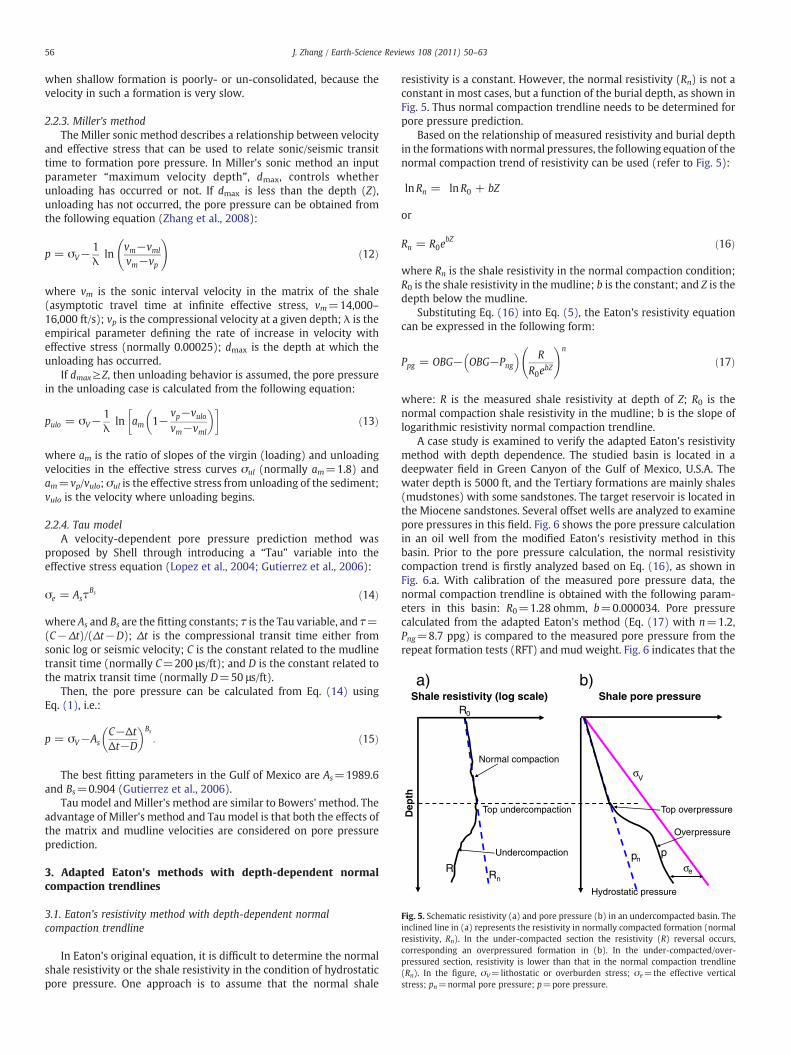
Fig. 5. Schematic resistivity (a) and pore pressure (b) in an undercompacted basin. Theinclined line in (a) represents the resistivity in normally compacted formation (normalresistivity, Rn). In the under-compacted section the resistivity (R) reversal occurs,corresponding an overpressured formation in (b). In the under-compacted/over-pressured section, resistivity is lower than that in the normal compaction trendline(Rn). In the figure, σV=lithostatic or overburden stress; σe=the effective verticalstress; pn=normal pore pressure; p=pore pressure.

56 J. Zhang / Earth-Science Reviews 108 (2011) 50–63

when shallow formation is poorly- or un-consolidated, because thevelocity in such a formation is very slow.

2.2.3. Miller's methodThe Miller sonic method describes a relationship between velocity

and effective stress that can be used to relate sonic/seismic transittime to formation pore pressure. In Miller's sonic method an inputparameter “maximum velocity depth”, dmax, controls whetherunloading has occurred or not. If dmax is less than the depth (Z),unloading has not occurred, the pore pressure can be obtained fromthe following equation (Zhang et al., 2008):

p = σV−1λ

lnvm−vml

vm−vp

!ð12Þ

where vm is the sonic interval velocity in the matrix of the shale(asymptotic travel time at infinite effective stress, vm=14,000–16,000 ft/s); vp is the compressional velocity at a given depth; λ is theempirical parameter defining the rate of increase in velocity witheffective stress (normally 0.00025); dmax is the depth at which theunloading has occurred.

If dmax≥Z, then unloading behavior is assumed, the pore pressurein the unloading case is calculated from the following equation:

pulo = σV−1λ

ln am 1−vp−vulovm−vml

� �� ð13Þ

where am is the ratio of slopes of the virgin (loading) and unloadingvelocities in the effective stress curves σul (normally am=1.8) andam=vp/vulo; σul is the effective stress from unloading of the sediment;vulo is the velocity where unloading begins.

2.2.4. Tau modelA velocity-dependent pore pressure prediction method was

proposed by Shell through introducing a “Tau” variable into theeffective stress equation (Lopez et al., 2004; Gutierrez et al., 2006):

σe = AsτBs ð14Þ

where As and Bs are the fitting constants; τ is the Tau variable, and τ=(C−Δt)/(Δt−D); Δt is the compressional transit time either fromsonic log or seismic velocity; C is the constant related to the mudlinetransit time (normally C=200 μs/ft); and D is the constant related tothe matrix transit time (normally D=50 μs/ft).

Then, the pore pressure can be calculated from Eq. (14) usingEq. (1), i.e.:

p = σV−AsC−ΔtΔt−D

� �Bs

: ð15Þ

The best fitting parameters in the Gulf of Mexico are As=1989.6and Bs=0.904 (Gutierrez et al., 2006).

Tau model andMiller's method are similar to Bowers' method. Theadvantage of Miller's method and Tau model is that both the effects ofthe matrix and mudline velocities are considered on pore pressureprediction.

3. Adapted Eaton's methods with depth-dependent normalcompaction trendlines

3.1. Eaton's resistivity method with depth-dependent normalcompaction trendline

In Eaton's original equation, it is difficult to determine the normalshale resistivity or the shale resistivity in the condition of hydrostaticpore pressure. One approach is to assume that the normal shale

resistivity is a constant. However, the normal resistivity (Rn) is not aconstant in most cases, but a function of the burial depth, as shown inFig. 5. Thus normal compaction trendline needs to be determined forpore pressure prediction.

Based on the relationship of measured resistivity and burial depthin the formations with normal pressures, the following equation of thenormal compaction trend of resistivity can be used (refer to Fig. 5):

lnRn = lnR0 + bZ

or

Rn = R0ebZ ð16Þ

where Rn is the shale resistivity in the normal compaction condition;R0 is the shale resistivity in the mudline; b is the constant; and Z is thedepth below the mudline.

Substituting Eq. (16) into Eq. (5), the Eaton's resistivity equationcan be expressed in the following form:

Ppg = OBG− OBG−Png� � R

R0ebZ

!n

ð17Þ

where: R is the measured shale resistivity at depth of Z; R0 is thenormal compaction shale resistivity in the mudline; b is the slope oflogarithmic resistivity normal compaction trendline.

A case study is examined to verify the adapted Eaton's resistivitymethod with depth dependence. The studied basin is located in adeepwater field in Green Canyon of the Gulf of Mexico, U.S.A. Thewater depth is 5000 ft, and the Tertiary formations are mainly shales(mudstones) with some sandstones. The target reservoir is located inthe Miocene sandstones. Several offset wells are analyzed to examinepore pressures in this field. Fig. 6 shows the pore pressure calculationin an oil well from the modified Eaton's resistivity method in thisbasin. Prior to the pore pressure calculation, the normal resistivitycompaction trend is firstly analyzed based on Eq. (16), as shown inFig. 6.a. With calibration of the measured pore pressure data, thenormal compaction trendline is obtained with the following param-eters in this basin: R0=1.28 ohmm, b=0.000034. Pore pressurecalculated from the adapted Eaton's method (Eq. (17) with n=1.2,Png=8.7 ppg) is compared to the measured pore pressure from therepeat formation tests (RFT) and mud weight. Fig. 6 indicates that the

0.1 1 10

Resistivity (ohmm)

Res shaleRes Rn

Dep

th (

ft b

elo

w s

ea f

loo

r)

Pore pressure gradient (ppg)

Pp ResOBGRFTMW

a) b)

0

1000

2000

3000

4000

5000

6000

7000

8000

9000

10000

11000

12000

13000

Dep

th (

ft b

elo

w s

ea f

loo

r)

0

1000

2000

3000

4000

5000

6000

7000

8000

9000

10000

11000

12000

13000

8 9 10 11 12 13 14 15 16 17 18

Fig. 6. Pore pressure calculated by adapted Eaton's resistivity method with depth-dependent compaction trendline in a deepwater post-well analysis in the Gulf of Mexico. The leftfigure (a) plots the resistivity in shale and the normal resistivity calculated from Eq. (16), and the resistivity is plotted in logarithmic scale. The right figure (b) shows the overburdenstress gradient (OBG), mud weight used while drilling (MW), measured pore pressure gradient (RFT) and pore pressure gradient (Pp Res) calculated from resistivity using Eq. (17).

Δt

Δtml

Δt (μμs/ft, log scale)

Top undercompaction

Abnormal pressure

Hydrostatic pressure

Pressure

Δtnp

pn σe

σv

40

Dep

th

240

Top overpressure

a) b)

Fig. 7. Schematic plots showing sonic transit time (Δt) measured in shale, the normalcompaction trend of the transit time in the normal pressure condition (Δtn) and thepore pressure response to the transit time (Δt).

57J. Zhang / Earth-Science Reviews 108 (2011) 50–63

formation is in normal compaction when depth is less than 4900 ftbelow the sea floor. Deeper than this depth (from 4900 to 7600 ft), theformation is slightly under-compacted with a lower resistivity thanthe normal compaction trend (Fig. 6.a), implying that the porepressure increases, as shown in Fig. 6.b. From 7600 to 13,000 ft, theformation is further under-compacted and more elevated porepressures exist. Fig. 6 demonstrates that the adapted Eaton'sresistivity method gives a fairly good result in pore pressurecalculation.

It should be noted that the pore pressure in the formation near thewellbore is affected by drilling-induced stresses (Zhang and Roegiers,2005). Therefore, in order to obtain the formation pore pressure thedeep resistivity is needed for the pore pressure calculation.

3.2. Eaton's velocity method with depth-dependent normal compactiontrendline

Slotnick (1936) recognized that the compressional velocity is afunction of depth, i.e., velocity increases with depth in the subsurfaceformations. Therefore, the normal compaction trendline of travel timeshould be a function of depth. The oldest and simplest normalcompaction trend of seismic velocity is a linear relationship given bySlotnick (1936) in the following form:

v = v0 + kZ ð18Þ

where v is the seismic velocity at depth of Z; v0 is the velocity in theground surface or at the sea floor; k is a constant.

Sayers et al. (2002) used this relationship as the normallypressured velocity for pore pressure prediction. A normal compactiontrend for shale acoustic travel time with depth in the Carnarvon Basinwas established by fitting an exponential relationship to averagedacoustic travel times from 17 normally pressured wells (van Ruth etal., 2004):

Δtn = 225 + 391e−0:00103Z ð19Þ

where Δtn is the acoustic transit time from the normal compactiontrend at the depth of investigation (μs/m); Z is in meters.

A similar relationship was used for a petroleum basin in Brunei(Tingay et al., 2009):

Δtn = 176:5 + 461:5e−0:0007Z: ð20Þ

Based on the data of the measured sonic transit time in theformations with normal pore pressures, as illustrated in Fig. 7, thefollowing general relationship of the normal compaction trend of thetransit time is proposed (refer to Appendix B for derivations):

Δtn = Δtm + Δtml−Δtmð Þe−cZ ð21Þ

where Δtm is the compressional transit time in the shale matrix (withzero porosity); Δtml is the mudline transit time; and c is the constant.

Substituting Eq. (21) into Eq. (6), the modified Eaton's sonicequation can be expressed in the following form:

Ppg = OBG− OBG−Png� � Δtm + Δtml−Δtmð Þe−cZ

Δt

!3

: ð23Þ

58 J. Zhang / Earth-Science Reviews 108 (2011) 50–63

The same case study, as presented in Section 3.1, is used toexamine the adapted Eaton's sonic transit time/velocity method. Fig. 8shows the determination of normal compaction trend of sonic transittime from Eq. (21) and pore pressure calculation using the Eaton'ssonic method with depth-dependent compaction trendline fromEq. (23). By calibrating the measured pore pressure data, the normalcompaction trend is determined from Eq. (21) with the followingparameters: Δtm=70 μs/ft, Δtml=200 μs/ft and c=0.000245. Com-pared to measured pore pressure data the pore pressure calculationfrom Eq. (23) (Fig. 8) gives a very good result.

4. New theoretical models of pore pressure prediction

4.1. Pore pressure prediction from porosity

As introduced before, the under-compaction is the primary reasonto cause formation overpressured, which occur primarily in rapidlysubsiding basins and in rocks with low permeability. The indicators ofunder-compaction are higher pore pressure and larger formationporosity than those in the normal compaction condition. It iscommonly accepted that porosity decreases exponentially as depthincreases in normally compacted formations (e.g., Athy, 1930):

ϕ = ϕ0e−cZ ð24Þ

where ϕ is porosity; ϕ0 is the porosity in the mudline; Z is the truevertical depth below themudline; c is the compaction constant in 1/mor 1/ft.

The same relationship exists in porosity and effective stress (e.g.,Dutta, 2002; Flemings et al., 2002; Peng and Zhang, 2007).

ϕ = ϕ0e−aσe ð25Þ

where a is the stress compaction constant in 1/psi or 1/MPa.As discussed previously, porosity is an indicator (a function) of

effective stress and pore pressure, particularly for the overpressuresgenerated from under-compaction and hydrocarbon cracking. There-fore, pore pressure can be estimated from formation porosity. Fig. 9illustrates how to identify under-compaction and overpressure fromporosity profile. When the porosity is reversal, the under-compaction

20 200

DT shaleDT normal

Transit time (μs/ft)

Dep

th (

ft b

elo

w s

ea f

loo

r)

0

1000

2000

3000

4000

5000

6000

7000

8000

9000

10000

11000

12000

13000

a)

Fig. 8. Pore pressure calculated by adapted Eaton's sonic velocity method with depth-dependthe sonic transit time in shale and the normal transit time calculated from Eq. (21), and the tr(OBG), mud weight used while drilling (MW), measured pore pressure (RFT) and pore pre

occurs and overpressure generates. The starting point of the porosityreversal is the top of under-compaction or top of overpressure. In theformation with under-compaction, porosity and pore pressure arehigher than those in the normally compacted one.

Efforts have been made to use porosity data for predicting porepressure in shales andmudstones. For instance, Holbrook et al. (2005)presented porosity-dependent effective stress for pore pressureprediction. Heppard et al. (1998) used an empirical porosity equationsimilar to Eaton's sonic method to predict pore pressure using shaleporosity data. Flemings et al. (2002) and Schneider et al. (2009) alsoapplied porosity–stress relationships to predict overpressures inmudstones.

The author derived a theoretical equation for pore pressureprediction from porosity according to normal compaction trend ofporosity (Zhang, 2008). The pore pressure gradient can be calculatedfrom the following equation (refer to Appendix A for derivations):

Ppg = OBG− OBG−Png� � lnϕ0− lnϕ

cZð26Þ

where ϕ is the porosity in shale at depth of Z, can be obtained fromsonic or density logs, ϕ0 is the porosity in the mudline (in the groundsurface or sea floor); Z is the depth below the mudline; c can beobtained from the normal compaction porosity trendline in Eq. (28).

From Eq. (26) the pore pressure, overburden stress and porosityhave the following relationship:

p = σV− σV−pnð Þ lnϕ0− lnϕcZ

: ð27Þ

The primary difference between Eq. (27) and other existing porepressure-porosity equations is that the pressures calculated fromEq. (27) are dependent on depths. In other words, the normalcompaction trendline of porosity is not a constant, but a function ofdepth.

When porosity (ϕ) at an interested depth is greater than thenormal porosity (ϕn) at the same depth, the formation has

8 9 10 11 12 13 14 15 16 17 18

OBGRFTMWPp DT

Pore pressure gradient (ppg)

Dep

th (

ft b

elo

w s

ea f

loo

r)

0

1000

2000

3000

4000

5000

6000

7000

8000

9000

10000

11000

12000

13000

b)

ent compaction trendline in a deepwater well in the Gulf of Mexico. The left figure plotsansit time is plotted in logarithmic scale. The right figure shows the overburden gradientssure gradient (Pp DT) calculated from sonic transit time using Eq. (23).

φ0

φn

φ

Porosity

Dep

th

Top overpressure

Abnormal pressure

Hydrostatic pressure

Pressure

σV

p

pn σe

a) b)

Fig. 9. Schematic porosity (a) and corresponding pore pressure (b) in a sedimentarybasin. The dash porosity profile in (a) represents normally compacted formation. In theoverpressured section the porosity reversal occurs (heavy line). In the overpressuredsection, porosity is larger than that in the normal compaction trendline (ϕn).

59J. Zhang / Earth-Science Reviews 108 (2011) 50–63

overpressure. The normal compaction porosity trendline can bedetermined from the following equation (rewritten from Eq. (24)):

ϕn = ϕ0e−cZ

: ð28Þ

4.2. Pore pressure prediction from transit time or velocity

Porosity (ϕ) in Eqs. (26) and (27) can be obtained from densityand sonic logs or from seismic interval velocity. The followingequation represents one of the methods to calculate porosity fromcompressional velocity/transit time proposed by Raiga-Clemenceau etal. (1988):

ϕ = 1− ΔtmΔt

� �1x ð29Þ

where x is the exponent to be determined from the data. In a study ofcompaction in siliciclastic rocks, predominantly shales, in theMackenzie Delta of northern Canada, Issler (1992) obtained labora-tory measurements of porosity in shales and determined a value of2.19 for the exponent x and used a fixed value of shale transit time,Δtm=67 μs/ft.

Substituting Eq. (29) into Eq. (26), the pore pressure can bepredicted from the compressional transit time/velocity, i.e.:

Ppg = OBG− OBG−Png� �Cm− ln 1− Δtm =Δtð Þ1=x

h icZ

ð30Þ

where Cm is the constant related to the compressional transit time inthe matrix and the transit time in the mudline, and Cm=ln[1−(Δtm/Δtml)1/x].

Porosity is often estimated by the empirical time average equationpresented by Wyllie et al. (1956):

ϕ =Δt−ΔtmΔtf−Δtm

ð31Þ

where Δtf is the transit time of interstitial fluids.

Substituting Wyllie's porosity-transit time equation into Eqs. (26)and (27), we obtain the following equations to calculate pore pressuregradient (Ppg) and pore pressure (p):

Ppg = OBG− OBG−Png� � ln Δtml−Δtmð Þ− ln Δt−Δtmð Þ

cZð32Þ

p = σV− σV−pnð Þ ln Δtml−Δtmð Þ− ln Δt−Δtmð ÞcZ

: ð33Þ

The normal compaction trendline of the transit time in Eqs. (32)and (33) can be obtained from the following equation (refer toAppendix B for derivations):

Δtn = Δtm + Δtml−Δtmð Þe−cZ: ð34Þ

This normal compaction trend allows the normal transit time toapproach the matrix transit time at a very large depth, which isphysically correct as Chapman (1983) pointed out. Unlike othermethods, this proposed sonic method (Eqs. (32), (33)) uses a normalcompaction trendline that is asymptotic to matrix transit time andtherefore better represents the compaction mechanism of thesediments. The other advantage of this model is that the calculatedpore pressures are dependent on depth, and both effects of the matrixand mudline transit time are considered.

4.3. Case applications

The proposed methods (porosity model in Eqs. (26), (27), andvelocity model in Eqs. (32), (33)) have been applied in severalpetroleum basins (e.g., in the Gulf of Mexico, North Sea and onshoreconventional gas and shale gas formations) to verify the applicability.Three examples of deepwater wells in the Gulf of Mexico arepresented in the following section.

4.3.1. Pore pressure from porosity modelThe same case study as shown in Figs. 6 and 8 is used in this section

for the comparison purpose. An important step in performing porepressure analysis is to select the clean shales in well log data. Prior toapplying the porosity model, one needs to obtain the shale porosityfrom density log or sonic log. Clay minerals have a crystallinestructure that can contain more radioactive elements than sand-stones. Therefore, gamma ray data in well logs can be used todifferentiate shale intervals from those of other lithologies. Drawingshale base lines in gamma ray data are the first step to identify andseparate shale from other rocks, as shown in Fig. 10. The high gammaray values (N75–110 API) are assumed to be pure shale, whereaspoints where gamma ray values are less than the shale base lines arenot used for analysis. Shale points defined on the gamma ray log arethen transferred to the corresponding sonic log or other logs used forpore pressure analysis (KSI, 2001).

Fig. 10 demonstrates how to obtain shale porosity from gamma rayand sonic logs. Porosity is calculated from the shale transit time fromWyllie's equation (Eq. (31)) using Δtf=200 μs/ft and Δtm=70 μs/ft.Using this porosity data, the normal compaction trend in porosity isanalyzed based on Eq. (28) with the parameters of ϕ0=0.8 andc=0.00024, as shown in Figs. 9.a and 11.a. Then, pore pressuregradient is calculated from the porosity model (Eq. (26)) withparameters obtained from Fig. 11.a (ϕ0=0.8, c=0.00024) andPng=8.7 ppg. The calculated pore pressure gradient is compared tothemeasured pore pressure from the repeat formation tests (RFT) andmud weight, as shown in Fig. 11.b. Compared to the pore pressure

Fig. 10. Log data and the calculated porosity from sonic transit time byWyllie's equation (Eq. (31)) in a deepwater well of the Gulf of Mexico. In this figure, the gamma ray and shalebase lines (SHBL) are shown in the left track; the sonic transit time (DT), shale points of the transit time (SHPT DT), and filtered shale transit time in shale (SHPT DT f21) are plotted inthe second track; and the calculated porosity from the filtered shale transit time is shown in the right track.

60 J. Zhang / Earth-Science Reviews 108 (2011) 50–63

obtained from the modified Eaton's sonic method (Fig. 8.b), theproposed porosity method (as shown in Fig. 11.b) gives a better resultin terms of matching measured pore pressures.

4.3.2. Pore pressure from sonic transit time modelThis case study presents another post-drill pore pressure analysis in

a Gulf of Mexico deepwater oil field with water depth of 3850 ft. Theformations are Tertiary shales and sandstones, and the target zone is

Porosity (unitless)

Porosity shalePorosity_normal

a)0 0.2 0.4 0.6 0.8 1

Dep

th (

ft b

elo

w s

ea f

loo

r)

0

1000

2000

3000

4000

5000

6000

7000

8000

9000

10000

11000

12000

13000

Fig. 11. Pore pressure prediction from the porosity method (Eq. (26)) using the data showcompaction trendline of porosity calculated from Eq. (28). The right track plots overburden(RFT), and pore pressure profile calculated from the porosity by Eq. (26) (Pp porosity).

located in the Middle Miocene sandstones. Fig. 12 shows a post-drillpore pressure analysis to examine the proposed sonic model. Porepressure gradient is calculated from proposed sonic equation (Eq. (32))using Δtml=200 μs/ft and Δtm=70 μs/ft, Png=8.75 ppg, and c=0.00028. The pore pressure gradient is also estimated using Bowers'method (Eq. (9)) with Δtml=200 μs/ft, Png=8.75 ppg, A=14,B=0.745. Compared to the result obtained from Bowers' method, theproposed method (Eq. (32)) gives a better result in pore pressure

Pore pressure gradient (ppg)

Pp porosityOBGRFTMW

b)

Dep

th (

ft b

elo

w s

ea f

loo

r)

8 9 10 11 12 13 14 15 16 17 180

1000

2000

3000

4000

5000

6000

7000

8000

9000

10000

11000

12000

13000

n in Fig. 8. The left track presents porosity of shales obtained from Fig. 10 and normalstress gradient (OBG), mud weight used while drilling (MW), measured pore pressure

DT shaleDT NCTL

Pp DT proposedOBGMDTMWPp DT Bowers

0

2000

4000

6000

8000

10000

12000

14000

16000

18000

20000

22000

40 80 120 160 200 240

Dep

th (

ft)

Sonic DT (μs/ft)

0

2000

4000

6000

8000

10000

12000

14000

16000

18000

20000

22000

8 9 10 11 12 13 14 15 16 17 18

Dep

th (

ft)

Pore pressure gradient (ppg)

Fig. 12. Pore pressure calculations from the sonic transit time method proposed in this paper (Eq. (32)) and from Bower's method. The left track presents the transit time of shalesobtained from sonic log and normal compaction trendline of transit time calculated from Eq. (34). The right track plots overburden stress gradient, mud weight used while drilling,measured pore pressure from MDT, and pore pressure profile calculated from the transit time by Eq. (32) and by Bower's method.

61J. Zhang / Earth-Science Reviews 108 (2011) 50–63

calculation, particularly in the shallow section, where other sonicmethods overestimate the pore pressures.

The proposed sonic method uses a normal compaction trendlineand the calculated pressures are dependent on depth. Therefore, thepore pressures in both shallow and deep depths can be betterpredicted.

Fig. 13. Pore pressure calculation from the sonic transit time proposed in this paper (Eq. (32and shale base lines are shown in the left track; the sonic transit time (DT) and filtered shalepore pressure from the filtered shale transit time (Pp DT) is shown in the right track with

4.3.3. Pore pressure from sonic transit time model in subsalt formationsPore pressure prediction is very challenging in subsalt formations

because the formationsmay be affected by salt with high salinity, thusa much lower resistivity. In addition, the salt tectonics may affect theformation compaction status, causing normal compaction trendchanges. Furthermore, the surface seismic survey cannot provide

)) in deepwater subsalt formations of the Gulf of Mexico. In this figure, the gamma raypoints of the transit time (SHPT DT) are plotted in the second track; and the calculatedcomparison to the measured formation pressures (MDT and Geotap).

62 J. Zhang / Earth-Science Reviews 108 (2011) 50–63

reliable interval velocities in the subsalt formations. Therefore, soniclog is critically important for pore pressure prediction while drilling.We examine a borehole drilled in a deepwater subsalt formations ofthe Gulf of Mexico. The field description can be found in Zhang et al.(2008). Pore pressure gradient is calculated from the proposed sonicequation (Eq. (32)) using Δtml=120 μs/ft and Δtm=73 μs/ft, Png=8.75 ppg and c=0.00009. Compared to the measured formationpressures, the proposed method (Eq. (32)) gives an excellent porepressure calculation in subsalt formations, as shown in Fig. 13. Itshould be noted that the mudline transit time needs to be adjusted(Δtml=120 μs/ft, instead of 200 μs/ft in conventional cases) to make abetter pore pressure estimation in subsalt formations.

5. Conclusions

For a hydraulically-connected/permeable aquifer or hydrocarbon-bearing formation (e.g., sandstone, limestone), the formation porepressure at the target depth can be calculated based on the differenceof the fluid column at the other depth where the pressure is known.However, in the formations of shales the pore pressures areoverpressured in the deep regions and the shales may not behydraulically connected. The pore pressures in shales cannot be easilyobtained from the fluid flow theory, because the overpressures areprimarily caused by compaction disequilibrium. Instead, well log orshale petrophysical data can be used to estimate the pore pressures inshales. Eaton's resistivity and sonic methods are adapted to provide amuch easier way to handle normal compaction trendlines. Theoreticalpore pressure-porosity model is the fundamental for pore pressureprediction in shales, where the compaction disequilibrium is theprimarymechanism of overpressure generation. Using this theoreticalmodel, pore pressure prediction from porosity and compressionalvelocity (sonic transit time) have been obtained. Case studies showthat pore pressures can be accurately obtained from well logging datausing correct methods with necessary calibrations.

Appendix A. Derivation of pore pressure prediction from porosity

It is well known that the formation porosity and effective stresshave the following relationship:

ϕ = ϕ0e−aσe ðA1Þ

Therefore, the effective stress can be obtained from Eq. (A1):

σe =1a

lnϕ0

ϕðA2Þ

The effective stress at normal pressure condition can also beobtained from Eq. (A1), when the porosity is the normal porosity, acondition that formations are normally compacted, i.e.:

ϕn = ϕ0e−aσn ðA3Þ

σn =1a

lnϕ0

ϕnðA4Þ

Combining Eqs. (A2) and (A4), one has:

σe

σn=

lnϕ0− lnϕlnϕ0− lnϕn

ðA5Þ

or,

σe = σnlnϕ0− lnϕlnϕ0− lnϕn

ðA6Þ

If we assume the Biot coefficient α=1 in Eq. (1), then, the effectivestress and pore pressure have the following relationship:

p = σV−σe: ðA7Þ

Substituting Eq. (A6) into Eq. (A7) and noticing σn=σV−pn, wecan obtain pore pressure, overburden stress and porosity relationship:

p = σV− σV−pnð Þ lnϕ0− lnϕlnϕ0− lnϕn

ðA8Þ

where ϕn is the porosity in the condition of the formation with anormal compaction.

The normal compaction porosity can be obtained from thefollowing equation (Eq. (24)):

ϕn = ϕ0e−cZ

: ðA9Þ

Substituting Eq. (A9) into Eq. (A8), we obtain the pore pressureand porosity relationship:

p = σV− σV−pnð Þ lnϕ0− lnϕcZ

ðA10Þ

where p is the pore pressure; σV is the overburden stress; pn is thenormal pore pressure; ϕ is porosity in shale, ϕ0 is the porosity in themudline (the ground surface or sea floor); Z is the depth below themudline; and c is the constant.

The pore pressure gradient can be easily obtained from Eq. (A10).

Ppg = OBG− OBG−Png� � lnϕ0− lnϕ

cZðA11Þ

where Ppg is the pore pressure gradient; OBG is the overburden stressgradient; Png is the normal pressure gradient.

Appendix B. Derivation of sonic normal compaction equation

From Wyllie equation (i.e., Eq. (31)), the porosity at normalcompaction condition (ϕn) can be expressed as:

ϕn =Δtn−ΔtmΔtf−Δtm

: ðB1Þ

And the porosity in the mudline (ϕml) can be written as follows:

ϕml =Δtml−ΔtmΔtf−Δtm

: ðB2Þ

From Eq. (A9), we have the following relationship between thenormal porosity and mudline porosity:

ϕn = ϕmle−cZ

: ðB3Þ

Substituting Eqs. (B1) and (B2) into Eq. (B3), we can obtain thetransit time in the normal compaction trend, i.e.:

Δtn = Δtm + Δtml−Δtmð Þe−cZ: ðB4Þ

References

Athy, L.F., 1930. Density, porosity, and compaction of sedimentary rocks. AAPG Bull.14 (1), 1–24.

Biot, M.A., 1941. General theory of three-dimensional consolidation. J. Appl. Phys.12 (1), 155–164.

Bowers, G.L., 1995. Pore pressure estimation from velocity data; accounting foroverpressure mechanisms besides undercompaction. SPE Drilling and Completions,June, 1995, pp. 89–95.

63J. Zhang / Earth-Science Reviews 108 (2011) 50–63

Bowers, G.L., 2001. Determining an Appropriate Pore-Pressure Estimation Strategy,Paper OTC 13042.

Burrus, J., 1998. Overpressure models for clastic rocks, their relation to hydrocarbonexpulsion: a critical reevaluation. In: Law, B.E., Ulmishek, G.F., Slavin, V.I. (Eds.),Abnormal pressures in hydrocarbon environments: AAPG Memoir, 70, pp. 35–63.

Chapman, R.E., 1983. Petroleum geology. Elsevier.Daines, S.R., 1982. Prediction of fracture pressures for wildcat wells. JPT 34, 863–872.Davies, R.J., Swarbrick, R.E., Evans, R.J., Huuse, M., 2007. Birth of a mud volcano: East

Java, 29 May 2006. GSA Today 17 (2). doi:10.1130/GSAT01702A.1.Dickinson, G., 1953. Geological aspects of abnormal reservoir pressures in Gulf Coast

Louisiana. AAPG Bull. 37 (2), 410–432.Dodson, J.K., 2004. Gulf of Mexico ‘trouble time’ creates major drilling expenses.

Offshore 64 (1).Dutta, N.C., 2002. Geopressure prediction using seismic data: current status and the

road ahead. Geophysics 67 (6), 2012–2041.Eaton, B.A., 1968. Fracture Gradient Prediction and Its Application in Oilfield Operations

Paper SPE2163 JPT 25–32.Eaton, B.A., 1972. The Effect of Overburden Stress on Geopressures Prediction fromWell

Logs Paper SPE3719 JPT 929–934 Aug., 1972.Eaton, B.A., 1975. The Equation for Geopressure Prediction from Well Logs. Society of

Petroleum Engineers of AIME. paper SPE 5544.Flemings, P.B., Stump, B.B., Finkbeiner, T., Zoback, M., 2002. Flow focusing in

overpressured sandstones: theory, observations, and applications. Am. J. Sci. 302,827–855.

Gardner, G.H.F., Gardner, L.W., Gregory, A.R., 1974. Formation velocity and density —

the diagnostic basis for stratigraphic traps. Geophysics 39 (6), 2085–2095.Gutierrez, M.A., Braunsdore, N.R., Couzens, B.A., 2006. Calibration and ranking of pore-

pressure prediction models. The leading Edge, Dec., 2006, pp. 1516–1523.Haimson, B.C., Fairhurst, C., 1970. In situ stress determination at great depth by means

of hydraulic fracturing. In: Somerton, W.H. (Ed.), Rock Mechanics — Theory andPractice. Am. Inst. Mining. Eng., pp. 559–584.

Heppard, P.D., Cander, H.S., Eggertson, E.B., 1998. Abnormal pressure and theoccurrence of hydrocarbons in offshore eastern Trinidad, West Indies. In: Law,B.E., Ulmishek, G.F., Slavin, V.I. (Eds.), Abnormal Pressures in HydrocarbonEnvironments: AAPG Memoir, 70, pp. 215–246.

Holand, P., Skalle, P., 2001. Deepwater Kicks and BOP Performance. SINTEF Report forU.S. Minerals Management Service.

Holbrook, P.W., Maggiori, D.A., Hensley, R., 2005. Real-time pore pressure and fracturegradient evaluation in all sedimentary lithologies. SPE Form. Eval. 10 (4), 215–222.

Hottmann, C.E., Johnson, R.K., 1965. Estimation of formation pressures from log-derivedshale properties Paper SPE1110 JPT 17, 717–722.

Hubbert, M.K., Willis, D.G., 1957. Mechanics of hydraulic fracturing. Pet. Trans. AIME210, 153–163.

Issler, D.R., 1992. A new approach to shale compaction and stratigraphic restoration,Beaufort-Mackenzie Basin and Mackenzie Corridor, Northern Canada. AAPG Bull.76, 1170–1189.

KSI, 2001. Best practice procedures for predicting pre-drill geopressures in deep waterGulf of Mexico. DEA Project 119 Report Knowledge Systems Inc.

Lang, J., Li, S., Zhang, J., 2011. Wellbore stability modeling and real-time surveillance fordeepwater drilling to weak bedding planes and depleted reservoirs. SPE/IADC139708 presented at the SPE/IADC Drilling Conference and Exhibition held inAmsterdam, The Netherlands, 1–3 March 2011.

Law, B.E., Spencer, C.W., 1998. Abnormal pressures in hydrocarbon environments. In:Law, B.E., Ulmishek, G.F., Slavin, V.I. (Eds.), Abnormal Pressures in HydrocarbonEnvironments: AAPG Memoir, 70, pp. 1–11.

Lopez, J.L., Rappold, P.M., Ugueto, G.A., Wieseneck, J.B., Vu, K., 2004. Integrated sharedearth model: 3D pore-pressure prediction and uncertainty analysis. The LeadingEdge, Jan., 2004, pp. 52–59.

Matthews, W.R., Kelly, J., 1967. How to predict formation pressure and fracturegradient. Oil Gas J. 65, 92–106.

Meng, Z., Zhang, J., Wang, R., 2011. In-situ stress, pore pressure and stress-dependentpermeability in the Southern Qinshui Basin. Int. J. Rock Mech. Min. Sci. 48 (1),122–131.

Morley, C.K., King, R., Hillis, R., Tingay, M., Backe, G., 2011. Deepwater fold and thrustbelt classification, tectonics, structure and hydrocarbon prospectivity: a review.Earth-Sci. Rev. 104, 41–91.

Mouchet, J.-C., Mitchell, A., 1989. Abnormal Pressures while Drilling. Editions TECHNIP,Paris.

Nelson, H.N., Bird, K.J., 2005. Porosity-depth Trends and Regional Uplift Calculated fromSonic Logs, National Reserve in Alaska. Scientific Investigation Report 2005–5051U.S. Dept. of the Interior and USGS.

Peng, S., Zhang, J., 2007. Engineering Geology for Underground Rocks. Springer.Powley, D.E., 1990. Pressures and hydrogeology in petroleum basins. Earth-Sci. Rev. 29,

215–226.Raiga-Clemenceau, J., Martin, J.P., Nicoletis, S., 1988. The concept of acoustic formation

factor for more accurate porosity determination from sonic transit time data. LogAnalyst 29 (1), 54–60.

Sayers, C.M., Johnson, G.M., Denyer, G., 2002. Predrill pore pressure prediction usingseismic data. Geophysics 67, 1286–1292.

Schneider, J., Flemings, P.B., Dugan, B., Long, H., Germaine, J.T., 2009. Overpressure andconsolidation near the seafloor of Brazos-Trinity Basin IV, northwest deepwaterGulf of Mexico. J. Geophys. Res. 114, B05102.

Slotnick, M.M., 1936. On seismic computation with applications. Geophysics 1, 9–22.Swarbrick, R.E., Osborne, M.J., 1998. Mechanisms that generate abnormal pressures: an

overview. In: Law, B.E., Ulmishek, G.F., Slavin, V.I. (Eds.), Abnormal Pressures inHydrocarbon Environments: AAPG Memoir, 70, pp. 13–34.

Swarbrick, R.E., Osborne, M.J., Yardley, G.S., 2002. Comparison of overpressuremagnitude resulting from the main generating mechanisms. In: Huffman, A.R.,Bowers, G.L. (Eds.), Pressure Regimes in Sedimentary Basins and their Prediction:AAPG Memoir, 76, pp. 1–12.

Terzaghi, K., Peck, R.B., Mesri, G., 1996. Soil Mechanics in Engineering Practice, 3 rdEdition. John Wiley & Sons.

Tingay, M.R.P., Hillis, R.R., Swarbrick, R.E., Morley, C.K., Damit, A.R., 2009. Origin ofoverpressure and pore-pressure prediction in the Baram province, Brunei. AAPGBull. 93 (1), 51–74.

Traugott, M., 1997. Pore pressure and fracture gradient determinations in deepwater.World Oil, August, 1997.

van Ruth, P., Hillis, R., Tingate, P., 2004. The origin of overpressure in the Carnarvon Basin,Western Australia: implications for pore pressure prediction. Pet. Geosci. 10, 247–257.

Wyllie, M.R.J., Gregory, A.R., Gardner, L.W., 1956. Elastic wave velocities inheterogeneous and porous media. Geophysics 21, 41–70.

Yardley, G.S., Swarbrick, R.E., 2000. Lateral transfer: a source of additional overpres-sure? Mar. Pet. Geol. 17, 523–537.

York, P., Prithard, D., Dodson, J.K., Dodson, T., Rosenberg, S., Gala, D., Utama, B., 2009.Eliminating non-productive time associated drilling trouble zone. OTC20220Presented at the 2009 Offshore Tech. Conf. Held in Houston.

Zhang, J., 2008. Unpublished reports and training notes.Zhang, J., Roegiers, J.-C., 2005. Double porosity finite element method for borehole

modeling. Rock Mech. Rock Eng. 38, 217–242.Zhang, J., Roegiers, J.-C., 2010. Discussion on “Integrating borehole-breakout di-

mensions, strength criteria, and leak-off test results, to constrain the state of stressacross the Chelungpu Fault, Taiwan”. Tectonophysics 492, 295–298.

Zhang, J., Standifird, W.B., Lenamond, C., 2008. Casing ultradeep, ultralong salt sectionsin deep water: a case study for failure diagnosis and risk mitigation in record-depthwell. Paper SPE 114273 Presented at SPE Annual Technical Conference andExhibition, 21–24 September 2008, Denver, Colorado, USA.