1-s2.0-S002072250200143X-main

Dynamic aspects of electroosmotic flow in a cylindricalmicrocapillary

Yuejun Kang, Chun Yang *, Xiaoyang Huang

School of Mechanical and Production Engineering, Nanyang Technological University,

50 Nanyang Avenue, 639798 Singapore

Received 11 June 2002; accepted 7 August 2002

(Communicated by E.S. S�UHUBI)

Abstract

Dynamic aspects of the electroosmotic flow (EOF) in a cylindrical capillary are analysed. An analytical

solution for electrostatic potential of the double layer has been derived by solving the complete Poisson–

Boltzmann equation for arbitrary zeta-potentials under an analytical scheme. Transient EOFfield in response

to the application of time dependent electric field is obtained analytically by using Green�s function method.

Specifically, sinusoidally alternating (AC) electric fields are used to study the effect of frequency-dependent

oscillation on the EOF. Limiting cases of zero frequency and pulsed electric field are also discussed.

� 2002 Published by Elsevier Science Ltd.

Keywords: Dynamic electroosmotic flow; Oscillating microchannel flow; AC electric field; Boltzmann distribution;

Cylindrical capillary

1. Introduction

Electroosmosis refers to the relative motion of polar media adjacent to a charged solid surfaceunder the application of a tangential electric field. Generally, most surfaces acquire a certainamount of electrostatic charges when they are brought into contact with a polar medium. Suchsurface charges, in turn, cause both counter-ions and co-ions in the liquid to be preferentiallyredistributed, leading to the formation of an electric double layer (EDL) [1]. Conceptually, theEDL can be divided into an inner compact layer and an outer diffuse layer. The inner layer,usually of several Angstroms, is immediately next to the charged surface and contains a layer of

*Corresponding author. Tel.: +65-6790-4883; fax: +65-6791-1859.

E-mail address: [email protected] (C. Yang).

0020-7225/02/$ - see front matter � 2002 Published by Elsevier Science Ltd.

PII: S0020-7225(02)00143-X

International Journal of Engineering Science 40 (2002) 2203–2221www.elsevier.com/locate/ijengsci

mail to: [email protected]

immobile counter-ions that are strongly attracted to the surface. In contrast, ions in the diffuselayer are less affected by the charged surface and are mobile. Within the diffuse layer, the counter-ions predominate and hence the local net charge density is not zero. Application of an externalelectric field tangentially to the EDL field would exert an electric body force on the ions in thediffuse layer, resulting in a net migration of the ions in the EDL region. The moving ions pulladjacent liquid with them to cause a bulk electroosmotic flow (EOF).

Electroosmosis has a variety of applications in technological processes such as membraneseparation, dewatering the waste sludge and removing poisonous heavy metal ions from soils inenvironmental remediation [2–4]. In addition, electroosmosis is being extensively employed in theBioMEMS technology as a transporting mode to control liquids such as pumping, valving,mixing, splitting etc and to delivery solute samples of nanovolumes in microfluidics used forchemical and biological analyses and medical diagnoses [5–7]. Compared with conventionallaboratory-sized instrumentation, the BioMEMS technology offers numerous advantages in-cluding higher throughput, faster analyses, smaller consumption of sample amount, and loweroperation and manufacturing costs.

In the literature, a vast majority of studies have been reported on the steady state EOF inmicrocapillaries of various geometric domains such as slit parallel plate [8], cylindrical capillary[9,10], annulus [11,12], elliptical pore [13,14], rectangular microchannel [15,16], and T and Ymicrochannel cross-sections [17–19]. In contrast, the transient aspects of the EOF have receivedrelatively less attention. It should be pointed out that study of unsteady EOF not only can providemore insights into the characteristics of EOF but also is important to the practical developmentand operation of the BioMEMS. According to Fan and Harrison [20], the efficiency of elec-trophoretic separation is strongly dependent on the duration of electroosmotic injection, which inturn is related to the evolution of the EOF. To reduce the contributions due to injection plugwidth and Joule heating, Jacobson et al. [21] proposed a high-speed electrophoretic separationmode to achieve the separation process within sub-milliseconds. Because of such order of mag-nitude of the time involved, model development should account for the dynamic effect of the EOF.Considering slow mixing processes occurred in microfluidics due to low Reynolds numberdominated laminar flow, Oddy et al. [22] designed an electrokinetic unstable mixer using fluctu-ating electric fields. In their experiments an instability of EOF driven by sinusoidally alternatingelectric fields was observed. On the theoretical side, S€ooderman and J€oonsson [23] developed atheoretical framework describing the temporal resolution of the EOF in both planar and cylin-drical geometries under the effect of pulsed electric fields. Using slip velocity approach, Satiago[24] studied the effects of fluid inertial and pressure on transient EOFs in a parallel plate. The slipvelocity model was first proposed by Overbeek [25] who showed that for microchannels withrelatively thin EDL thickness, the flow field outside the double layer is an irrotational flow witha slip velocity boundary condition determined by the well-known Helmholtz–Smoluchowskiequation. Without assumption of the thin EDL thickness, Keh and Tseng [26] obtained an ana-lytical solution for the transient electrokinetic flow in a capillary tube and a capillary slit. Ex-clusively, aforementioned theoretical analyses however were based on the Debye–H€uuckel linearapproximation, which is valid only for low zeta potentials. Using a complete numerical approach,Yang et al. [27] simultaneously solved coupled Poisson equation, Nernst–Planck equation, andfull Navier–Stokes equation to study the time and space development of EOF in a two-parallelplate microchannel.

2204 Y. Kang et al. / International Journal of Engineering Science 40 (2002) 2203–2221

The current paper presents an in depth analysis of the dynamics of EOF in a cylindrical mi-crocapillary. We start with the time evolution of the transient EOF motivated by a time dependentelectric field, and discuss the flow field oscillations excited by a sinusoidally alternating electricfield. Importantly, the complete Poisson–Boltzmann equation governing the EDL electric field isanalytically solved with arbitrary zeta potentials under a proposed analytical scheme. The validityof the Boltzmann distribution is discussed. Exact solutions for transient velocity distributions andtime-dependent mean velocities are obtained using the Green�s function method. As a compari-son, the solution under slip velocity approximation is also presented.

2. Dynamics of electroosmotic flow

2.1. Formulation of the problem

Consider an EOF in a cylindrical capillary of radius a. The liquid in the microcapillary is as-sumed to be an incompressible, Newtonian, symmetric monovalence electrolyte of density, q, andviscosity, l. The capillary wall is uniformly charged with the zeta potential, f0. When an externalelectric field, EðtÞ is applied along the axis of the capillary, the liquid starts to move as result of theinteraction between the net charge density in the EDL and the applied electric field. The motion ofliquid through the cylindrical microcapillary is governed by the Navier–Stokes equation [4]

qouðr; tÞ

ot� l

1

ro

orrouðr; tÞ

or

� �¼ EðtÞqeðrÞ ð1Þ

where uðr; tÞ is the transient velocity field. qeðrÞ is the local volumetric net charge density of theelectrolyte due to the presence of the EDL, and in combination of the Boltzmann distribution(a proof of the validity of the Boltzmann distribution will be presented in the next section), itis expressed as

qeðrÞ ¼ e0ðnþ � n�Þ ¼ �2n0e0 sinhe0wðrÞkT

� �ð2Þ

where e0 is the elementary charge, n0 is the ionic concentration in the bulk phase (i.e., far from thecharged surfaces), k is the Boltzmann constant, T is the absolute temperature, and wðrÞ is theelectric potential of the EDL.

Introducing the following dimensionless parameters:

�uu ¼ uus

�tt ¼ lqa2

t �rr ¼ ra

W ¼ e0wkT

ð3Þ

We can non-dimensionalize Eqs. (1) and (2) respectively as

o�uuo�tt

� 1

�rro

o�rr�rro�uuo�rr

!¼ a2

lusqeð�rrÞEð�ttÞ ð4Þ

Y. Kang et al. / International Journal of Engineering Science 40 (2002) 2203–2221 2205

and

qeð�rrÞ ¼ �2n0e0 sinh½Wð�rrÞ� ð5Þ

Here us is the reference velocity defined as

us ¼ � ere0l

E0f0 ð6Þ

where er is the dielectric constant of the electrolyte and e0 is the permittivity of vacuum. Thereference velocity, us can also be regarded as the ‘‘slip’’ velocity on the shear plane of the EDL[25]. Obviously, us is proportional to the magnitude of the external field, E0 and the zeta potential,f0.

Substituting Eq. (5) into Eq. (4), we obtain

o�uuo�tt

� 1

�rro


!¼ ðja2Þ

WsE0

sinh½Wð�rrÞ�Eð�ttÞ ð7Þ

where Ws ¼ e0f0=kT and j ¼ ð2n0e20=ere0kT Þ1=2

. j is the Debye–H€uuckel parameter, and 1=j denotesthe characteristic thickness of the EDL. Eq. (7) is subject to the initial and boundary conditions

�tt ¼ 0 �uu ¼ 0 ð8aÞ

�rr ¼ 0o�uuo�rr

¼ 0 �rr ¼ 1 �uu ¼ 0 ð8bÞ

Eq. (7) can be classified as a 2nd order inhomogeneous diffusion equation. In the following, ananalytical solution will be sought by using the Green�s function approach to obtain the dynamicEOF field activated by the time-dependent electric fields.

2.2. Green’s function of inhomogeneous diffusion equation

According to the Green�s function method [28], the general solution of inhomogeneous diffu-sion equation

ouot

� Dr2u ¼ Qðx; tÞ ð9Þ

is given by

uðx; tÞ ¼Z t

0

Z Z ZGðx; t; n; sÞQðn; sÞdnds þ

Z Z ZGðx; t; n; 0Þuðn; 0Þdn

þ aZ t

0

ZZ

Gðx; t; n; sÞ ouon

�� uðn; sÞ oG

on

�dS ds ð10Þ


where Gðx; t; n; sÞ is the Green�s function of the specified diffusion equation, i.e., Eq. (9). Thesecond and third terms on the right hand side represent the effects of initial and boundary con-ditions, respectively.

The corresponding problem of Eqs. (7)–(8b) for determining the Green�s function Gðr; tjn; sÞshould satisfy [29]

oGo�tt

� 1

�rro

o�rr�rroGo�rr

� �¼ dð�rr � nÞdð�tt � sÞ ð11Þ

subject to the initial and boundary conditions

Gð�rr; 0jn; sÞ ¼ 0 ð12aÞ

o

orGð0;�ttjn; sÞ ¼ 0 ð12bÞ

Gð1;�ttjn; sÞ ¼ 0 ð12cÞ

where dð�rr � nÞ and dð�rr � sÞ are Dirac delta functions. We can see that the source is an impulse at�tt ¼ s, located at �rr ¼ n. G then gives the description of effect of this impulse as it propagates awayfrom �rr ¼ n in the course of time.

Taking Hankel transform with respect to �rrðGH ¼ HfGgÞ and using the boundary conditionsEqs. (12b) and (12c), we obtain

dGH

d�ttþ k2

nGH ¼ nJ0ðknnÞdð�tt � sÞ ð13Þ

where kn are the positive roots of the zero-order Bessel function J0ðknÞ ¼ 0.Now, we take the Laplace transform with respect to �ttðGHL ¼ LfGHgÞ and use the initial con-

dition Eq. (12a) to obtain

sGHL þ k2nGHL ¼ nJ0ðknnÞe�ss ð14Þ

We solve for GHL and get

GHL ¼ nJ0ðknnÞsþ k2

n

e�ss ð15Þ

Taking inverse Laplace transform of Eq. (15) gives

GH ¼ Hð�tt � sÞnJ0ðknnÞe�k2nð�tt�sÞ ð16Þ

where Hð�tt � sÞ is the Heaviside step function.Further, the inversion with respect to Hankel transform leads to

Gð�rr;�ttjn; sÞ ¼ Hð�tt � sÞX1n¼1

2J0ðkn�rrÞJ 21 ðknÞ

nJ0ðknnÞ exp½�k2nð�tt � sÞ� ð17Þ


According to Eq. (10), using the initial and boundary conditions given in Eqs. (8a) and (8b) wecan show that the solution to Eq. (7) is expressed as

�uuð�rr;�ttÞ ¼Z �tt

s¼0

Z 1

n¼0

Gð�rr;�ttjn; sÞ ðjaÞ2

WsE0

sinh½WðnÞ�EðsÞ( )

dnds ð18Þ

Substituting Eq. (17) into Eq. (18) leads to

�uuð�rr;�ttÞ ¼ 2ðjaÞ2

Ws

X1n¼1

CnJ0ðkn�rrÞJ 21 ðknÞ

Z �tt

s¼0

1

E0

EðsÞ exp½�k2nð�tt � sÞ�ds ð19Þ

where Cn ¼R 1

n¼0nJ0ðknnÞ sinh½WðnÞ�dn.

Integrating Eq. (19) along the radius of the cylinder, we obtain the non-dimensional meanvelocity

�uumð�ttÞ ¼ 2

Z 1

�rr¼0

�rr�uuð�rr;�ttÞd�rr ¼ 4ðjaÞ2

Ws

X1n¼1

Cn1

knJ1ðknÞ

Z �tt

s¼0

1

E0

EðsÞ exp½�k2nð�tt � sÞ�ds ð20Þ

2.3. Special cases

2.3.1. Sinusoidally alternating electric field

Consider the application of a sinusoidally alternating electric field with an angle frequency x

EðtÞ ¼ E0eixt ð21Þ

Substituting Eq. (21) into Eq. (19), we can show next

�uuð�rr;�ttÞ ¼ REAL2ðjaÞ2

Ws

X1n¼1


expðib2�ttÞ � expð�k2n�ttÞ

k2n þ ib2

" #

¼ 2ðjaÞ2

Ws

X1n¼1


k2n cosðb

2�ttÞ þ b2 sinðb2�ttÞ � k2n expð�k2

n�ttÞ

k4n þ b4

ð22Þ

where i is the unit imaginary number. ‘‘REAL’’ denotes the real part of the solution. Here a newparameter b is defined as [30]

b ¼ affiffiffiffiffiffiffiffiffiffiffiffil=qx

p ð23Þ

b represents the aspect ratio of the capillary radius a to the Stokes penetration depth ds, defined as[30]


ds ¼ffiffiffiffiffiffiffil

qx

r¼

ffiffiffiffiffiffiffiffiffiffiffil

2pqf

rð24Þ

where f ¼ x=2p is the frequency of the applied electric field.Accordingly, the mean velocity is given by

�uumð�ttÞ ¼ 2

Z 1

�rr¼0

�rr � �uuð�rr;�ttÞd�rr

¼ 4ðjaÞ2

Ws

X1n¼1

Cn1

knJ1ðknÞk2n cosðb

2�ttÞ þ b2 sinðb2�ttÞ � k2n expð�k2

n�ttÞ

k4n þ b4

ð25Þ

2.3.2. Step change electric fieldThe external electric field is applied and remains constant from the time t ¼ 0 (i.e., the electric

field follows step function change)

EðtÞ ¼ E0HðtÞ ð26Þ

where

Hðt � dÞ ¼ 1 ðt > dÞ0 ðt < dÞ

�ð27Þ

is the well-known Heaviside step function.Substituting Eq. (26) into Eqs. (19) and (20), we obtain


Ws

X1n¼1


1� expð�k2n�ttÞ

k2n

ð28Þ

and

�uumð�ttÞ ¼4ðjaÞ2

Ws

X1n¼1

Cn1� expð�k2

n�ttÞ

k3nJ1ðknÞ

ð29Þ

In fact, we also can derive Eqs. (28) and (29) by setting the angle frequency of the electrical field xin Eqs. (22) and (25) equal to zero, and then b ¼ 0. Hence Eqs. (22) and (25) can reduce to Eqs.(28) and (29), respectively.

2.4. Square wave electric field

For a more general situation when the electric field is switched on at the time t ¼ 0 and remainsconstant until it is switched off at the time t ¼ d, the electric field is then described by

E ¼ E0 � ½HðtÞ �Hðt � dÞ� ð30Þ


Substituting Eq. (30) to Eqs. (19) and (20), we get


Ws

X1n¼1


exp½�k2nð�tt � �ddÞ �Hð�tt � �ddÞ� � expð�k2

n�ttÞ

k2n

ð31Þ

and

�uumð�ttÞ ¼4ðjaÞ2

Ws

X1n¼1

Cnexp½�k2

nð�tt � �ddÞ �Hð�tt � �ddÞ� � expð�k2n�ttÞ

k3nJ1ðknÞ

ð32Þ

The total volumetric net flow quantity from the electric field is switched on to the termination ofthe entire flow due to frictional stress can be determined from

�QQVð�ddÞ ¼Z 1

�tt¼0

�uumð�ttÞd�tt ¼ �dd � 4ðjaÞ2

Ws

X1n¼1

Cn1

k3nJ1ðknÞ

ð33Þ

It is obvious that the total net flow quantity is proportional to the duration of time �dd (here�dd ¼ ðl=qa2Þd), during which the electric field is applied.

3. Boltzmann distribution and electric double layer field

In the following, we will first present the validation of the Boltzmann distribution under theEOF considered in the current study. As clearly shown in Eq. (1), it is through the electrical bodyforce term that the Navier–Stokes equation is coupled with the governing equation for the EDLfield, which in turn is associated with ionic number concentration distribution, ni. Generally,rigorous mathematical modelling of ion transport in the EDL region under an EOF generated bysinusoidally alternating electric fields should take into account of unsteady effects. According tothe literature, the time scale related to electromigration in the EDL is of order 10�8–10�7 s [31];this value is at least two orders smaller than the characteristic time associated with the evolutionof the EOF, which is of order 10�5–10�3 s [32]. In the present study, we concern the sinusoidallyalternating electric field of the highest frequency as 500 KHz (see the discussion part), corre-sponding to a characteristic time of 2� 10�6 s. Therefore, the transient effect of the EDL ‘‘re-laxation’’ can safely be neglected, and the ionic concentration distribution niðr) in themicrochannel EOF follows the Nernst–Planck equation [33], which in the absence of chemicalreactions takes the convective-diffusion form

r � ðDirniÞ � r � ðV i � niÞ ¼ 0 ð34Þ

where Di is the diffusion coefficient of the type-i ion and V i is the velocity of the type-i ion. Undersuch a situation, the ion velocity, V i, can be decomposed into contributions from liquid hydro-dynamic velocity, V , and a velocity, Ui, due to electromigration (caused by the presence of theelectric field). Then we can write


V i ¼ V þ Ui ð35Þ

The velocity, Ui, is related to the electric forces exerting on the ions through the followingequation

F ei ¼ zie0E ¼ fiU i ð36Þ

where zi is the valence of the type-i ion, e is the elementary charge, and fi is the hydrodynamicresistance coefficient which can be determined from the Stokes–Einstein equation

fi ¼kTDi

ð37Þ

The local electric field, E is assumed to be decoupled as the summation of the applied electric fieldand the EDL field due to the charged channel wall, and thus E can be expressed as

E ¼ EðtÞez �rw ð38Þ

where EðtÞ is the applied electric field and exists only along the flowing axial direction, ez. w is theelectrical potential of the EDL field. Then from Eqs. (36)–(38), we can readily obtain an ex-pression for Ui

Ui ¼ ½EðtÞez �rw� zie0Di

kTð39Þ

Substituting Eqs. (35) and (39) into Eq. (34), and making use of continuity equationr � V ¼ 0, wecan show next

Dir2ni þr � zie0DinikT

rw

� �� V � rni �

zie0Di

kTEðtÞrni � ez ¼ 0 ð40Þ

When the microchannel EOF is fully developed, the components of fluid velocity V satisfyuz ¼ uzðr; tÞ and ur ¼ uh ¼ 0 in terms of cylindrical coordinates. Eq. (40) can reduce to

Dir2ni þr � zie0Dinikt

rw

� �� uz

�þ zie0Di

kTEðtÞ

�onioz

¼ 0 ð41Þ

Note that the ionic number concentration is time-independent and the flow is fully-developed,implying no appreciable ionic concentration gradient is established along the flow direction, i.e.,oni=oz ¼ 0. Then Eq. (41) becomes

Dir2ni þr � zie0DinikT

rw

� �¼ 0 ð42Þ


We can readily solve Eq. (42), and obtain its solution, which is

ni ¼ ni0 exp�� zie0w

kT

�ð43Þ

Here ni0 is the ionic number concentration of the type-i ions in the bulk phase where w ¼ 0. Eq.(43) is the well-known Boltzmann distribution. Therefore, it can be concluded that for a micro-channel EOF in a fully developed condition, the equilibrium Boltzmann distribution is still valid ifthe frequency of the external electric field is not very high, (e.g., less than 1 MHz).

Consequently, the EDL potential distribution, wðrÞ within the capillary region can be describedby Poisson–Boltzmann equation which, in polar coordinates, takes the non-dimensional form [1]

1

Rd

dRRdWðRÞdR

� �¼ sinhWðRÞ ð44Þ

Eq. (44) is subject to the following boundary conditions

WðjaÞ ¼ Ws

dWðRÞdR

��R¼0

¼ 0 ð45Þ

where R ¼ jr.However, no exact solution to Eq. (44) is available because of non-linearity. In this work, we

follow Philip and Wooding [34] to approximate the hyperbolic sine function sinh W as

sinhW �� 1

2expð�WÞ W < �1

W �16W6 112expðWÞ W > 1

8><>: ð46Þ

Such an analytical scheme was successfully used by Philip and Wooding [34] in their studyconcerning the electrical potential distribution outside a charged cylindrical particle immersed inan electrolyte. They found that the obtained potential profile differs only slightly from that byusing numerical integration of the complete P–B equation.

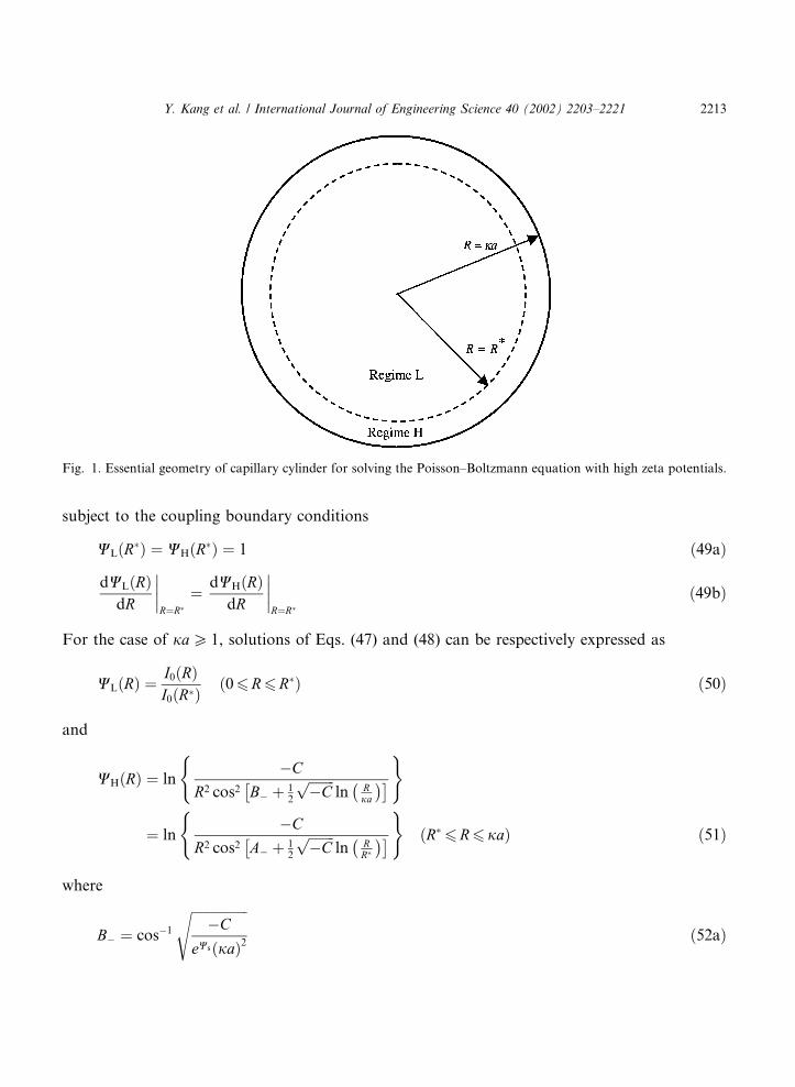
Based on the analytical scheme given in Eq. (46), we envisage the entire cylindrical region ascomprising two hypothetical concentric regimes (L and H) so that at their junctions (i.e., R ¼ R�),we have W ¼ 1 (see Fig. 1). Hence we propose to solve the following equations:

Low potential regime L ð06R6R�Þ

1

Rd

dRRdWLðRÞ

dR

� �¼ WLðRÞ ð47Þ

High potential regime H ðR�6R6 jaÞ

1

Rd

dRRdWHðRÞ

dR

� �¼ 1

2exp½WHðRÞ� ð48Þ


subject to the coupling boundary conditions

WLðR�Þ ¼ WHðR�Þ ¼ 1 ð49aÞ

dWLðRÞdR

��R¼R�

¼ dWHðRÞdR

��R¼R�

ð49bÞ

For the case of jaP 1, solutions of Eqs. (47) and (48) can be respectively expressed as

WLðRÞ ¼I0ðRÞI0ðR�Þ ð06R6R�Þ ð50Þ

and

WHðRÞ ¼ ln�C

R2 cos2 B� þ 12

ffiffiffiffiffiffiffiffi�C

pln R

ja

� �� ( )

¼ ln�C

R2 cos2 A� þ 12


pln R

R�

� �� ( )

ðR�6R6 jaÞ ð51Þ

where

B� ¼ cos�1

ffiffiffiffiffiffiffiffiffiffiffiffiffiffiffiffiffi�C

eWsðjaÞ2

sð52aÞ

Fig. 1. Essential geometry of capillary cylinder for solving the Poisson–Boltzmann equation with high zeta potentials.


A� ¼ cos�1

ffiffiffiffiffiffiffiffiffi�CeR�2

r¼ B� þ 1

2


pln

R�

ja

� �ð52bÞ

I0 is the first kind, zero-order modified Bessel function. C is the integration constant, determinedby

C ¼ 2

�þ R� I1ðR�Þ

I0ðR�Þ

�2� eR�2 ð53Þ

4. Results and discussion

In calculations, NaCl is used as the electrolyte solution. At room temperature of T ¼ 298 K, theelectrolyte properties are dielectric constant er ¼ 80, viscosity l ¼ 0:90� 10�3 kg/m s, and densityq ¼ 998 kg/m3.

4.1. Potential profile

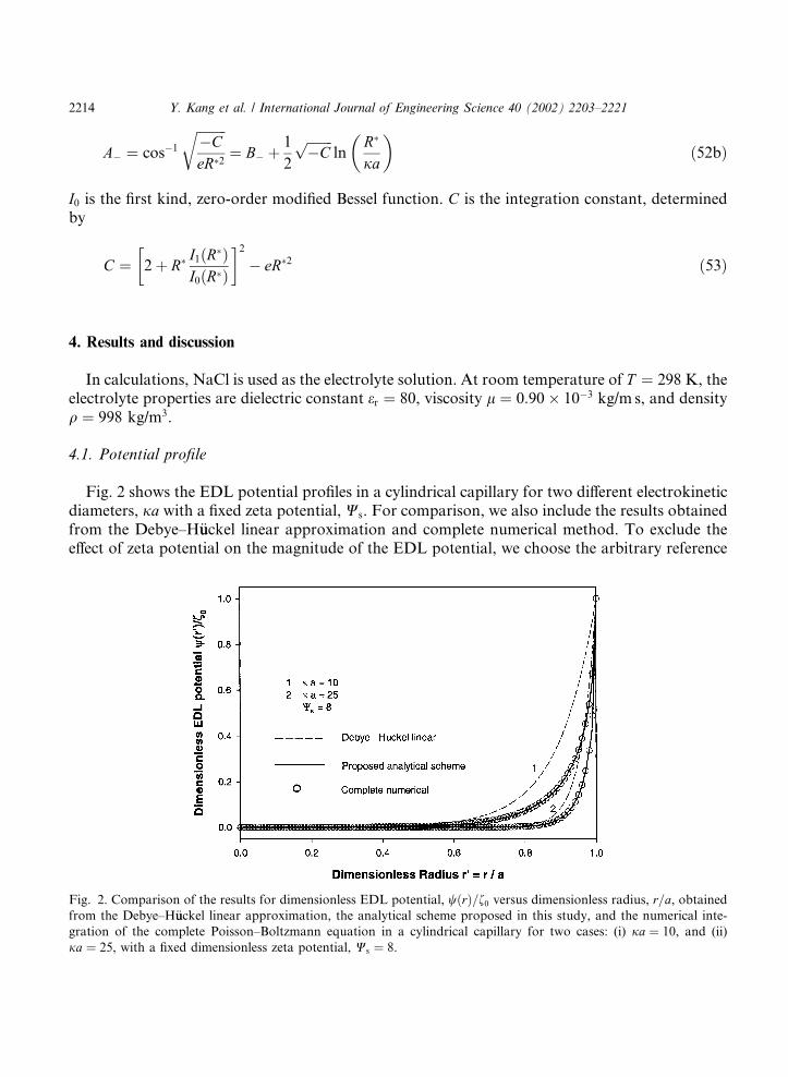
Fig. 2 shows the EDL potential profiles in a cylindrical capillary for two different electrokineticdiameters, ja with a fixed zeta potential, Ws. For comparison, we also include the results obtainedfrom the Debye–H€uuckel linear approximation and complete numerical method. To exclude theeffect of zeta potential on the magnitude of the EDL potential, we choose the arbitrary reference

Fig. 2. Comparison of the results for dimensionless EDL potential, wðrÞ=f0 versus dimensionless radius, r=a, obtainedfrom the Debye–H€uuckel linear approximation, the analytical scheme proposed in this study, and the numerical inte-

gration of the complete Poisson–Boltzmann equation in a cylindrical capillary for two cases: (i) ja ¼ 10, and (ii)

ja ¼ 25, with a fixed dimensionless zeta potential, Ws ¼ 8.


potential, f0. It is shown in Fig. 2 that the Debye–H€uuckel linear assumption provides a goodapproximation for a larger electrokinetic diameter. However, the linearized solution deviates fromthe complete Poisson–Boltzmann equation for a smaller electrokinetic diameter, i.e., a thickerEDL corresponding to a dilute electrolyte or smaller capillary. Furthermore, it is noted from Fig.2 that the difference between the analytical scheme used in the present study and the numericalsolution of the Poisson–Boltzmann equation is visually indistinguishable, suggest an excellentapproximation estimated by Eq. (46).

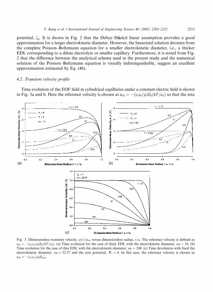
4.2. Transient velocity profile

Time evolution of the EOF field in cylindrical capillaries under a constant electric field is shownin Fig. 3a and b. Here the reference velocity is chosen as us0 ¼ �ðere0=lÞE0ðkT=e0Þ so that the zeta

Fig. 3. Dimensionless transient velocity, uðrÞ=us0 versus dimensionless radius, r=a. The reference velocity is defined as

us0 ¼ �ðere0=lÞE0ðkT=e0Þ. (a) Time evolution for the case of thick EDL with the electrokinetic diameter, ja ¼ 10. (b)

Time evolution for the case of thin EDL with the electrokinetic diameter, ja ¼ 100. (c) Time devolution with fixed the

electrokinetic diameter, ja ¼ 32:57 and the zeta potential, Ws ¼ 4. In this case, the reference velocity is chosen as

us0 ¼ �ðere0=lÞE0f0.


potential effect can be shown. According to the results displayed in Fig. 3a and b, we can observethat upon the application of an electric field, the flow is activated in a region adjacent to thechannel wall and the velocity increases rapidly from zero on the wall to a maximum within theEDL where the driving force is present. As the time goes, the flow gradually extends to the restportion of the channel due to hydrodynamic stresses originated from liquid viscosity. When theflow in entire channel becomes steady, the flow velocity across the channel other than the EDLregion remains almost a constant value, resembling a plug flow. Furthermore, we can estimate thecharacteristic time scale for the EOF to reach its steady state from Eq. (28) by choosingk21�tt� ¼ k2

1ðl=qa2Þt� ¼ 1. Then we can obtain t� ¼ qa2=lk21, where k1 ¼ 2:405 determined from

J0ðknÞ ¼ 0; this shows that the characteristic time, t� is proportional to the square of the channelradius, a2. In addition, it is noted that the velocity increases with the increasing zeta potential,indicating an almost linear relationship between the velocity and the zeta potential.

As a comparison, when the electric field is switched off the time devolution of the EOF is shownin Fig. 3c. It can be seen that the flow decays following a parabolic trend, and is similar to thewell-known Stokes first problem, i.e., a streaming flow over a suddenly stopped plate, which wasdiscussed in length by Telionis [30]. However, such a similarity is not coincidence. As pointed outearlier, the EOF is activated inside the EDL, which can be considered as the moving plate in theStokes first problem. Once the ‘‘driving force’’ is removed––the moving plate is suddenly stoppedand the external electric field is turned off, the mechanism governing fluid flow is the same, i.e.,hydrodynamic frictional stresses due to liquid viscosity.

4.3. AC perturbation

For a capillary of a ¼ 10 lm in radius, we can estimate the characteristic time for the EOF toreach a steady state is t� ¼ qa2=lk2

1 ¼ 19:2 ls. The corresponding eigenfrequency of the system isf � ¼ 1=t� ¼ lk2

1=qa2 ¼ 52:25 kHz. Hence, three different characteristic frequencies of the external

electric field, 0:1f �, f � and 10f �ðf ¼ x=2pÞ are chosen to study the characteristic features of theoscillating EOF.

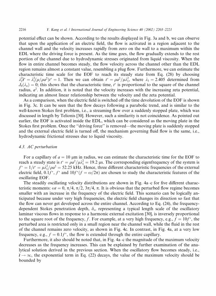
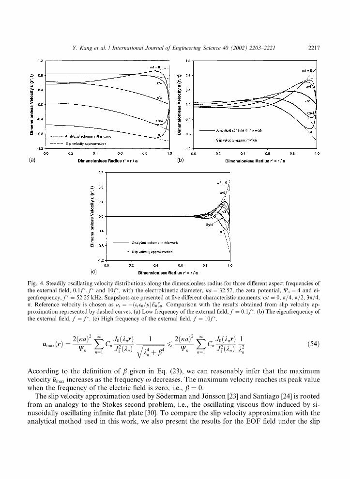
The steadily oscillating velocity distributions are shown in Fig. 4a–c for five different charac-teristic moments: xt ¼ 0, p=4, p=2, 3p=4, p. It is obvious that the perturbed flow regime becomessmaller with an increase in the frequency of the electric field. This scenario can be logically an-ticipated because under very high frequencies, the electric field changes its direction so fast thatthe flow can never get developed across the entire channel. According to Eq. (24), the frequency-dependent Stokes penetration depth, ds, representing a typical length scale of the oscillatorylaminar viscous flows in response to a harmonic external excitation [30], is inversely proportionalto the square root of the frequency, f . For example, at a very high frequency, e.g., f ¼ 10f �, theperturbed area is restricted only in a small region near the channel wall, while the fluid in the restof the channel remains zero velocity, as shown in Fig. 4c. In contrast, in Fig. 4a, at a very lowfrequency, e.g., f ¼ 0:1f �, the flow is extended through the entire capillary.

Furthermore, it also should be noted that, in Fig. 4a–c the magnitude of the maximum velocitydecreases as the frequency increases. This can be explained by further examination of the ana-lytical solution derived in the previous section. When the oscillatory flow becomes steady, i.e.,�tt ! 1, the exponential term in Eq. (22) decays, the value of the maximum velocity should bebounded by


�uumaxð�rrÞ ¼2ðjaÞ2

Ws

X1n¼1


1ffiffiffiffiffiffiffiffiffiffiffiffiffiffiffik4n þ b4

q 62ðjaÞ2

Ws

X1n¼1


1

k2n

ð54Þ

According to the definition of b given in Eq. (23), we can reasonably infer that the maximumvelocity �uumax increases as the frequency x decreases. The maximum velocity reaches its peak valuewhen the frequency of the electric field is zero, i.e., b ¼ 0.

The slip velocity approximation used by S€ooderman and J€oonsson [23] and Santiago [24] is rootedfrom an analogy to the Stokes second problem, i.e., the oscillating viscous flow induced by si-nusoidally oscillating infinite flat plate [30]. To compare the slip velocity approximation with theanalytical method used in this work, we also present the results for the EOF field under the slip

Fig. 4. Steadily oscillating velocity distributions along the dimensionless radius for three different aspect frequencies of

the external field, 0:1f �; f � and 10f �, with the electrokinetic diameter, ja ¼ 32:57, the zeta potential, Ws ¼ 4 and ei-

genfrequency, f � ¼ 52:25 kHz. Snapshots are presented at five different characteristic moments: xt ¼ 0, p=4, p=2, 3p=4,p. Reference velocity is chosen as us ¼ �ðere0=lÞE0f0. Comparison with the results obtained from slip velocity ap-

proximation represented by dashed curves. (a) Low frequency of the external field, f ¼ 0:1f �. (b) The eigenfrequency of

the external field, f ¼ f �. (c) High frequency of the external field, f ¼ 10f �.


velocity approximation, represented by dashed curves in Fig. 4a–c. Detailed derivation of theelectroosmotic velocity with the slip velocity approximation is provided in Appendix. It is dem-onstrated in Fig. 4a–c that at the center region of the capillary, the two methods give nearly thesame results for transient velocity distributions, while adjacent to the charged channel wall thediscrepancy is observed. Such a discrepancy is due to the assumption of moving boundary con-dition used in the slip velocity approximation, in which the boundary velocity is assumed to beproportional to the oscillating electric field (refer to Eq. (A.2c)), while the boundary velocity is

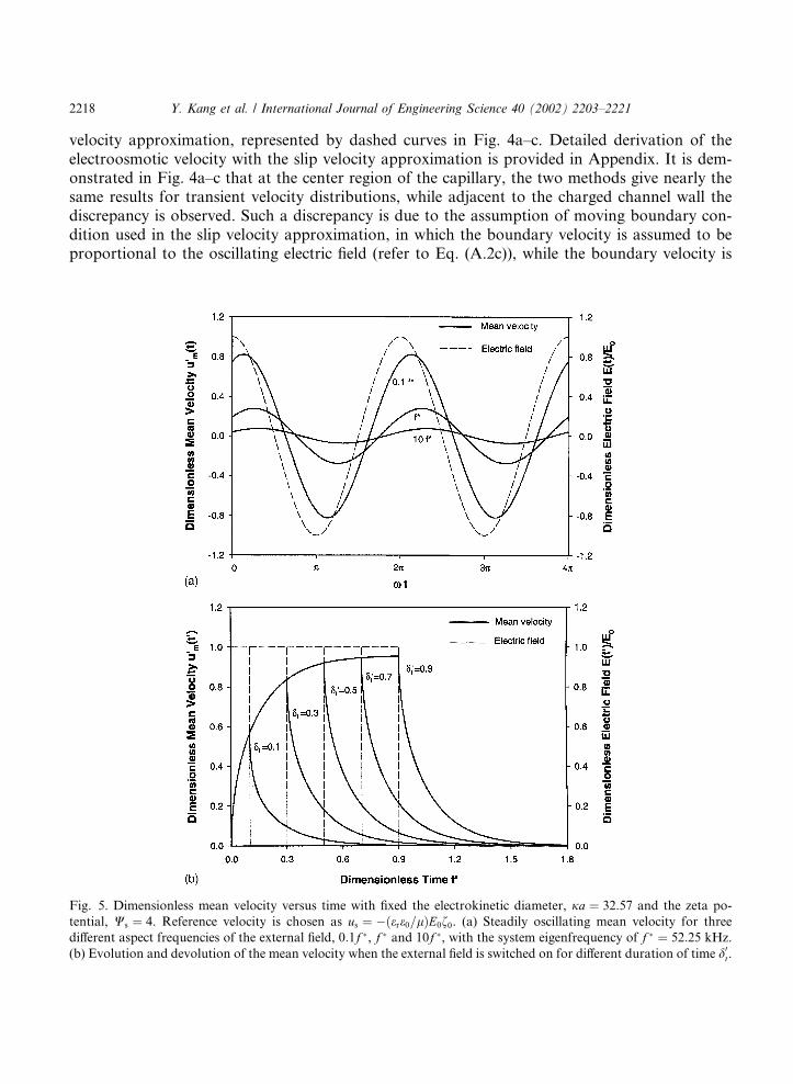
Fig. 5. Dimensionless mean velocity versus time with fixed the electrokinetic diameter, ja ¼ 32:57 and the zeta po-

tential, Ws ¼ 4. Reference velocity is chosen as us ¼ �ðere0=lÞE0f0. (a) Steadily oscillating mean velocity for three

different aspect frequencies of the external field, 0:1f �, f � and 10f �, with the system eigenfrequency of f � ¼ 52:25 kHz.

(b) Evolution and devolution of the mean velocity when the external field is switched on for different duration of time d0t.


chosen as zero (i.e., no-slip condition) in the analytical scheme used in present study. The slipvelocity approximation neglects the velocity profile in the EDL region. Thus the analytical schemeused in this work can present a more accurate and complete scenario for the oscillating EOF in themicrochannel.

In Fig. 5a, the time dependent mean velocity is plotted for two-cycle periods of the AC electricfield. The flow can follow the sinusoidally oscillation of the electric field, but there exists a phaselag. The phase lag is larger as the frequency goes higher. For the same reason as the maximumtransient velocity, the magnitude of the maximum mean velocity is also dependent on the fre-quency.

�uummax ¼4ðjaÞ2

Ws

X1n¼1

Cn1

knJ1ðknÞ1ffiffiffiffiffiffiffiffiffiffiffiffiffiffiffi

k4n þ b4

q 64ðjaÞ2

Ws

X1n¼1

Cn1

k3nJ1ðknÞ

ð55Þ

Fig. 5b shows dependence of the mean EOF velocity on the time, during which the electric fieldis powered on. It is shown that the flow cannot reach its steady state until the time is larger thanthe characteristic time. On the other hand, the flow decays exponentially after the electric field isswitched off.

5. Conclusion

An analytical scheme is used to solve the Poisson–Boltzmann equation for study of thedynamics of EOF in a cylindrical microcapillary. The results show that the solution of thePoisson–Boltzmann equation based on the analytical scheme is virtually no different fromnumerical solution. It is demonstrated that the geometry and zeta potential of the channel wallhave a strong impact on the EOF. The electrokinetic diameter determines the relative thickness ofthe EDL while zeta potential determines the magnitude of the velocity, and hence the flow rate.The characteristic time for the flow to reach its steady state is proportional to the square of thechannel radius. The evolution of the EOF upon application of a constant electric field exhibits aunique flow profile, which is resulted from the contributions due to the electric body force andhydrodynamic viscous stress. On the other hand, the flow devolution after the external electricfield is switched off follows a flow pattern solely controlled by hydrodynamic friction due to liquidviscosity. In addition, it is found that the oscillating EOF is strongly dependent on the modulationfrequency of the applied sinusoidally alternating electric field, which determines the thickness ofunstable Stokes layer, and thus governs the extent of the harmonic oscillation and the velocitydistributions of the oscillating EOF. The results obtained from this work not only can provideinsights into the EOF but also can furnish a guidance for the design and development of the ACelectrokinetic micromixers and micropumps.

Acknowledgement

YJK wishes to gratefully acknowledge the Ph.D. scholarship from Nanyang TechnologicalUniversity.


Appendix A. Slip velocity approximation in AC perturbation

Conceptually, the steadily oscillating velocity profile induced by the application of a sinusoi-dally alternating electric field is similar to the fluid flow induced by an oscillating motion of thechannel wall; the latter was well documented by Telionis [30]. The basic concept of introducing theslip velocity approximation is to neglect the thin EDL region such that the entire flow is motivatedby the frictional stresses originated from liquid viscosity. Here the thin EDL region can be re-garded as an oscillating moving channel wall. The outer slip boundary velocity is determined bythe Helmholtz–Smoluchowski equation, usðtÞ ¼ �ðere0=lÞf0E0e

ixt. Hence the harmonically oscil-lating flow field is governed by the Navier–Stokes equation, in non-dimensional form

o�uuo�tt

¼ 1

�rro


!ðA:1Þ

subject to the initial and boundary conditions (the reference velocity used in non-dimensionli-zation is chosen as us ¼ �ðere0=lÞE0f0)

�tt ¼ 0 �uu ¼ 0 ðA:2aÞ

�rr ¼ 0o�uuo�rr

¼ 0 ðA:2bÞ

�rr ¼ 1 �uu ¼ expðib2�ttÞ ðA:2cÞ

Solution to Eq. (A.1) can be readily obtained by using the classical method of separation ofvariables, and it is given as

�uuð�rr;�ttÞ ¼ REALI0ð

ffiffii

pb�rrÞ

I0ðffiffii

pbÞ

expðib2�ttÞ" #

ðA:3Þ

where I0 is the zero-order modified Bessel function of the first kind, and i is the unit imaginarynumber. ‘‘REAL’’ denotes the real part of the solution.

References

[1] R.J. Hunter, Zeta Potential in Colloid Science: Principles and Applications, Academic Press, New York, 1981.

[2] V.M. Barragan, C.R. Bauza, Electroosmotic through a cation-exchange membrane: effect of an ac perturbation on

the electroosmotic flow, J. Colloid Interf. Sci. 230 (2000) 359.

[3] R.A. Jacobs, R.F. Probstein, Two-dimensional modelling of electroremediation, AICHE J. 42 (1996) 1685.

[4] R.F. Probstein, Physicochemical Hydrodynamics: An Introduction, second ed., John Wiley & Sons, New York,

1994.

[5] D.J. Harrison, K. Fluri, K. Seiler, Z. Fan, C.S. Effenhauser, A. Manz, Micromachining a miniaturized capillary

electrophoresis-based chemical analysis system on a chip, Science 261 (1993) 895.

[6] A. Manz, C.S. Effenhauser, N. Burggraf, D.J. Harrison, K. Seiler, K. Fluri, Electroosmotic pumping and

electrophoretic separations for miniaturized chemical analysis systems, J. Micromech. Microeng. 4 (1994) 257.


[7] van den A. Berg, T.S.J. Lammerink, Micro total analysis systems: microfluidic aspects, integration concepts and

applications, Topics Curr. Chem. 194 (1998) 21.

[8] D. Burgreen, F.R. Nakache, Electrokinetic flow in ultrafine capillary slits, J. Phys. Chem. 68 (1964) 1084.

[9] C.L. Rice, R. Whitehead, Electrokinetic flow in narrow cylindrical capillaries, J. Phys. Chem. 69 (1965) 4017.

[10] S. Levine, J.R. Marriott, G. Neale, N. Epstein, Theory of electrokinetic flow in fine cylindrical capillaries at high

zeta potentials, J. Colloid Interf. Sci. 52 (1975) 136.

[11] H.K. Tsao, Electroosmotic flow through an annulus, J. Colloid Interf. Sci. 225 (2000) 247.

[12] Y.J. Kang, C. Yang, X.Y. Huang, Electroosmotic flow in a capillary annulus with high zeta potentials, J. Colloid

Interf. Sci., in press.

[13] W.H. Koh, J.L. Anderson, Electroosmotic and electrolyte conductance in charged microcapillaries, AICHE J. 21

(1975) 1176.

[14] J.P. Hsu, C.Y. Kao, S.J. Tseng, C.J. Chen, Electrokinetic flow through an elliptical microchannel: effects of aspect

ratio and electrical boundary conditions, J. Colloid Interf. Sci. 248 (2002) 176.

[15] C. Yang, D. Li, J.H. Masliyah, Modeling forced liquid convection in rectangular microchannels with electrokinetic

effects, Int. J. Heat Mass Transfer 41 (1998) 4229.

[16] S. Arulanandam, D. Li, Liquid transport in rectangular microchannels by electroosmotic pumping, Colloids Surf.

A 161 (2000) 89.

[17] N.A. Patankar, H.H. Hu, Numerical simulation of electroosmotic flow, Anal. Chem. 70 (1998) 1870.

[18] L. Hu, J. Harrison, J.H. Masliyah, Numerical model of electrokinetic flow for capillary electrophoresis, J. Colloid

Interf. Sci. 215 (1999) 300.

[19] F. Bianchi, R. Ferrigno, H.H. Girault, Finite element simulation of an electroosmotic-driven flow division at a

t-junction of microscale dimensions, Anal. Chem. 72 (2000) 1987.

[20] Z.H. Fan, J.D. Harrison, Micromachining of capillary electrophoresis injectors and separators on glass chips and

evaluation of flow at capillary intersections, Anal. Chem. 66 (1994) 177.

[21] S.C. Jacobson, R. Hergenroder, L.B. Koutny, J.M. Ramsey, High-speed separations on a microchip, Anal. Chem.

66 (1994) 1114.

[22] M.H. Oddy, J.G. Santiago, J.C. Mikkelsen, Electrokinetic instability micromixing, Anal. Chem. 73 (2001) 5822.

[23] O. S€ooderman, B. J€oonsson, Electro-osmosis: velocity profiles in different geometries with both temporal and spatial

resolution, J. Chem. Phys. 105 (1996) 10300.

[24] J.G. Santiago, Electroosmotic flows in microchannels with finite inertial and pressure forces, Anal. Chem. 73 (2001)

2353.

[25] J.Th.G. Overbeek, in: H.R. Kruyt (Ed.), Phenomenology of Lyophobic (Chapter II), Colloid Science, Amsterdam,

1952.

[26] H.J. Keh, H.C. Tseng, Transient electrokinetic flow in fine capillaries, J. Colloid Interf. Sci. 242 (2001) 450.

[27] R.J. Yang, L.M. Fu, C.C. Hwang, Electroosmotic entry flow in a microchannel, J. Colloid Interf. Sci. 244 (2001)

173.

[28] M.P. Morse, H. Feshbach, Methods of Theoretical Physics, McGraw-Hill Publishing Company, New York, 1953.

[29] E. Butkov, Mathematical Physics, Addison-Wesley Publishing Company, New York, 1968.

[30] D.P. Telionis, Unsteady Viscous Flow, Springer-Verlag, New York, 1981.

[31] J.P. Hsu, Y.C. Kuo, S.J. Tseng, Dynamic interactions of two electrical double layers, J. Colloid Interf. Sci. 195

(1997) 388.

[32] C. Yang, C.B. Ng, V. Chan, Transient analysis of electroosmotic flow in a slit microchannel, J. Colloid Interf. Sci.

248 (2002) 524.

[33] T.G.M. van de Ven, Colloidal Hydrodynamics, Academic Press, San Diego, 1989.

[34] J.R. Philip, R.A. Wooding, Solution of the Poisson–Boltzmann equation about a cylindrical particle, J. Chem.

Phys. 52 (1970) 953.


Documents

1-s2.0-S002072250200143X-main