Embed Size (px)
Citation preview
1
Section 5The Exchange Rate in the Short Run
2
Content
• Objectives• Aggregate Demand• Output Market Equilibrium• Asset Market Equilibrium • The Short-Run Equilibrium • Temporary Policy Changes• Permanent Policy Changes• The J-Curve• Summary
3
Objectives
• To understand the determinants of aggregate demand.
• To know how output is determined using aggregate demand and aggregate supply.
• To know the effects of fiscal and monetary policy.
• To know the J-curve
4
Aggregate Demand
• Aggregate demand comes from
• Aggregate demand is the amount of a country’s output demanded by throughout the world.
• It consists of – Consumption demand (C)– Investment demand (I)– Government demand (G)– Current account (CA)
IMEXGICD
5
Aggregate Demand
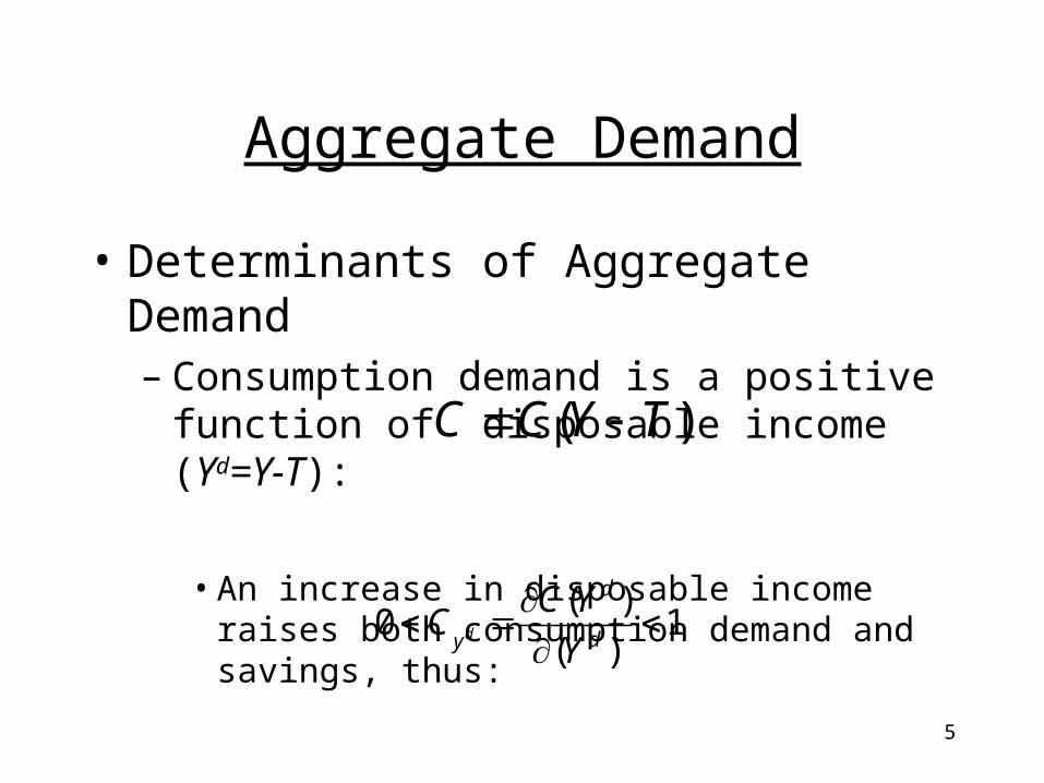
• Determinants of Aggregate Demand– Consumption demand is a positive function of
disposable income (Yd=Y-T):
• An increase in disposable income raises both consumption demand and savings, thus:
)( TYCC
1)(
)(0
d
d
y Y
YCC d
6
Aggregate Demand
– Investment demand is assumed to be exogenous for now. In more complex models, investment demand is a positive function of income and a negative function of the interest rate.
– Government demand is a policy variable. It is assumed exogenous.
7
Aggregate Demand
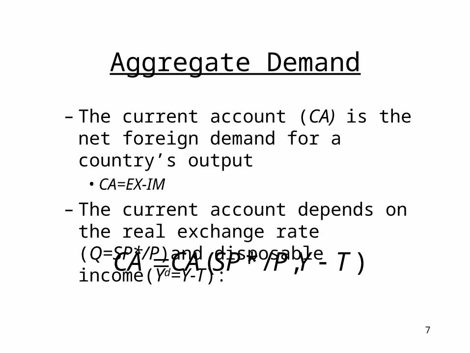
– The current account (CA) is the net foreign demand for a country’s output
• CA=EX-IM
– The current account depends on the real exchange rate (Q=SP*/P)and disposable income(Yd=Y-T):
),/*( TYPSPCACA
8
Aggregate Demand
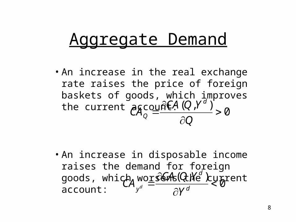
• An increase in the real exchange rate raises the price of foreign baskets of goods, which improves the current account:
• An increase in disposable income raises the demand for foreign goods, which worsens the current account:
0),(
Q
YQCACA
d
Q
0),(
d
d
y Y
YQCACA d
9
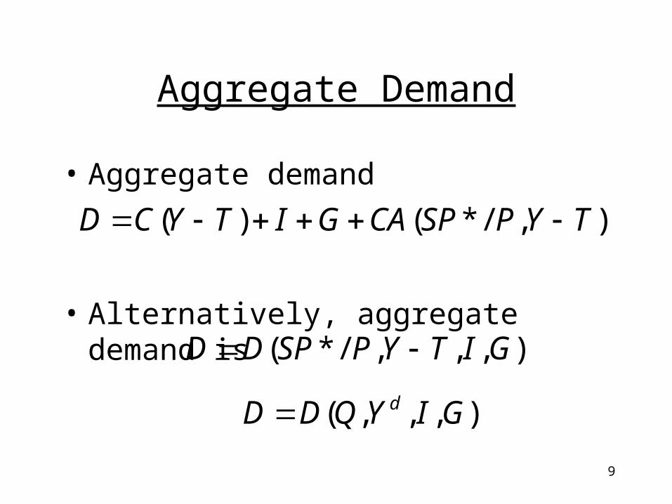
Aggregate Demand
• Aggregate demand
• Alternatively, aggregate demand is
),/*()( TYPSPCAGITYCD
),,,/*( GITYPSPDD
),,,( GIYQDD d
10
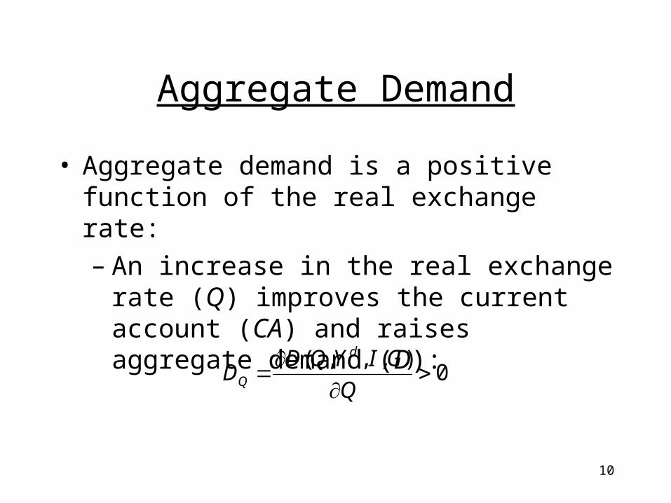
Aggregate Demand
• Aggregate demand is a positive function of the real exchange rate:– An increase in the real exchange rate (Q)
improves the current account (CA) and raises aggregate demand (D):
0),,,(
Q
GIYQDD
d
Q
11
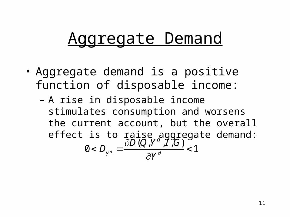
Aggregate Demand
• Aggregate demand is a positive function of disposable income:– A rise in disposable income stimulates consumption
and worsens the current account, but the overall effect is to raise aggregate demand:
1),,,(
0
d
d
Y Y
GIYQDD d
12
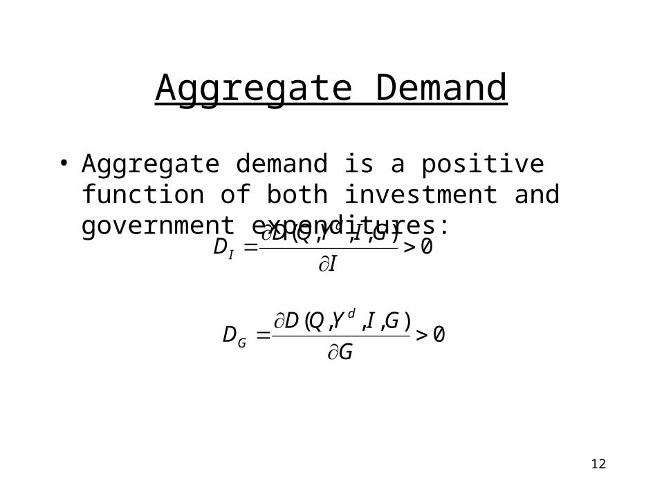
Aggregate Demand
• Aggregate demand is a positive function of both investment and government expenditures:
0),,,(
I
GIYQDD
d
I
0),,,(
G
GIYQDD
d
G
13
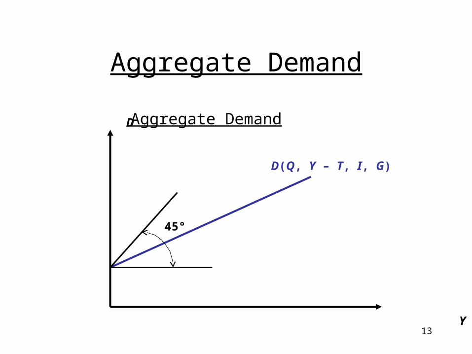
Aggregate Demand
Y
D
D(Q, Y – T, I, G)
45°
Aggregate Demand
14
Output Market Equilibrium
• The output market short-run equilibrium
),,,/*( GITYPSPDY
15
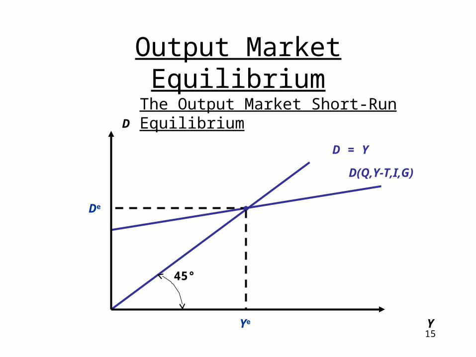
Output Market Equilibrium
D = Y
D(Q,Y-T,I,G)
Y
D
De
Ye
45°
The Output Market Short-Run Equilibrium
16
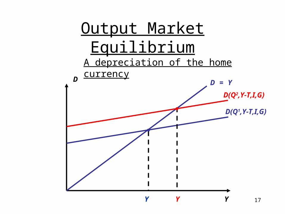
Output Market Equilibrium
• The effects of an increase in the real exchange rate:– With fixed prices, an increase in the nominal exchange
rate raises the real exchange rate (the relative price of a foreign basket of goods).
– This causes an upward shift in the aggregate demand function and an expansion of output.
17
Output Market Equilibrium
Y
D
D(Q1,Y-T,I,G)
D = Y
D(Q2,Y-T,I,G)
Y Y
A depreciation of the home currency
18
Output Market Equilibrium
• An increase in either investment or government expenditures also cause an upward shift in the aggregate demand function and an expansion of output.– The effects are similar to an increase in the
nominal exchange rate.
19
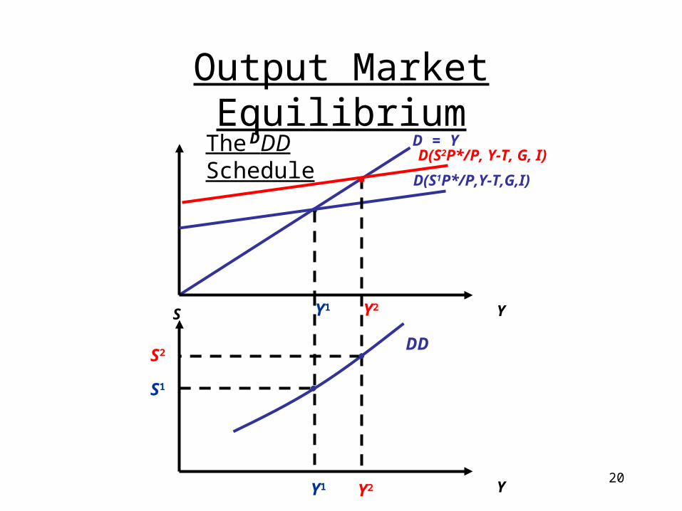
Output Market Equilibrium
• The DD schedule– It shows all the short-run equilibrium
combinations of output and the exchange rate that are consistent with the output market.
20
Output Market EquilibriumD = Y
Y
DD(S2P*/P, Y-T, G, I)
D(S1P*/P,Y-T,G,I)
Y1 Y2
Y
S
DD
Y1 Y2
S2
S1
The DD Schedule
21
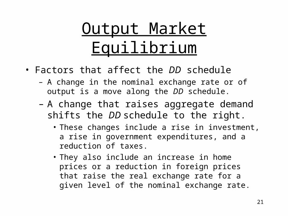
Output Market Equilibrium
• Factors that affect the DD schedule– A change in the nominal exchange rate or of output is a move
along the DD schedule.
– A change that raises aggregate demand shifts the DD schedule to the right.
• These changes include a rise in investment, a rise in government expenditures, and a reduction of taxes.
• They also include an increase in home prices or a reduction in foreign prices that raise the real exchange rate for a given level of the nominal exchange rate.
22
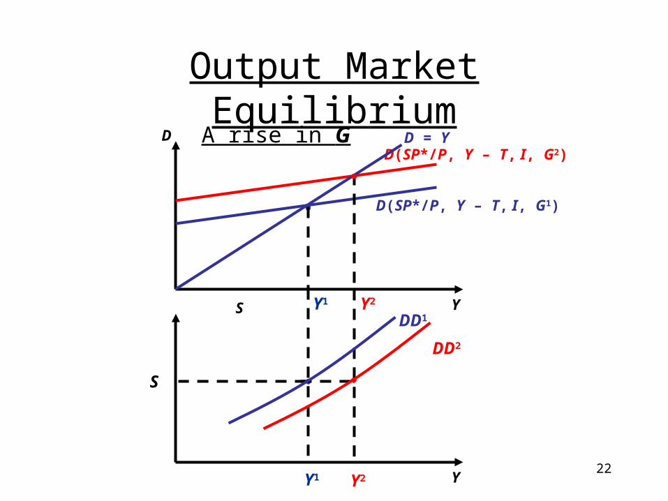
Output Market Equilibrium
Y
D
Y
S
D(SP*/P, Y – T, I, G2)
D(SP*/P, Y – T, I, G1)
D = Y
Y1 Y2
Y1 Y2
S
DD1
DD2
A rise in G
23
Asset Market Equilibrium
• The AA Schedule– It shows all the equilibrium combinations of
output and the exchange rate that are consistent with the home money market and the foreign exchange market.
24
Asset Market Equilibrium
– The AA schedule represents the asset market equilibrium
– It combines the money market equilibrium with the foreign exchange equilibrium (the uncovered interest parity condition).
• M/P = L(i,Y)
• i = i* + (Se – S)/S
25
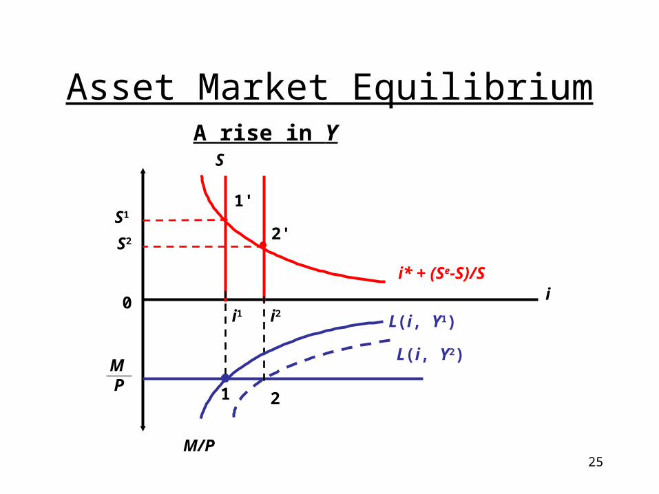
Asset Market Equilibrium
M/P
i
S
0i2
M P
i* + (Se-S)/S
1
i1
S1
S2 2'
2
1'
L(i, Y2)
L(i, Y1)
A rise in Y
26
Asset Market Equilibrium
• The equilibrium in asset markets requires:– A rise in output is related to an appreciation of the
domestic currency.
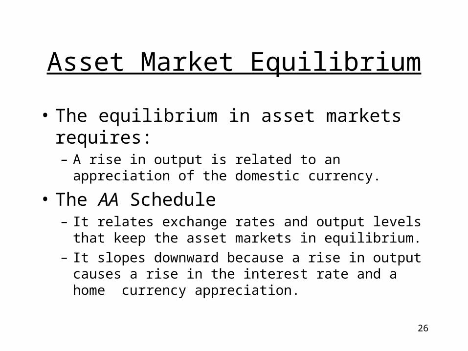
• The AA Schedule– It relates exchange rates and output levels that keep the
asset markets in equilibrium.
– It slopes downward because a rise in output causes a rise in the interest rate and a home currency appreciation.
27
Asset Market Equilibrium
Y
S
Y2
S22
Y1
S11
AA
The AA Schedule
28
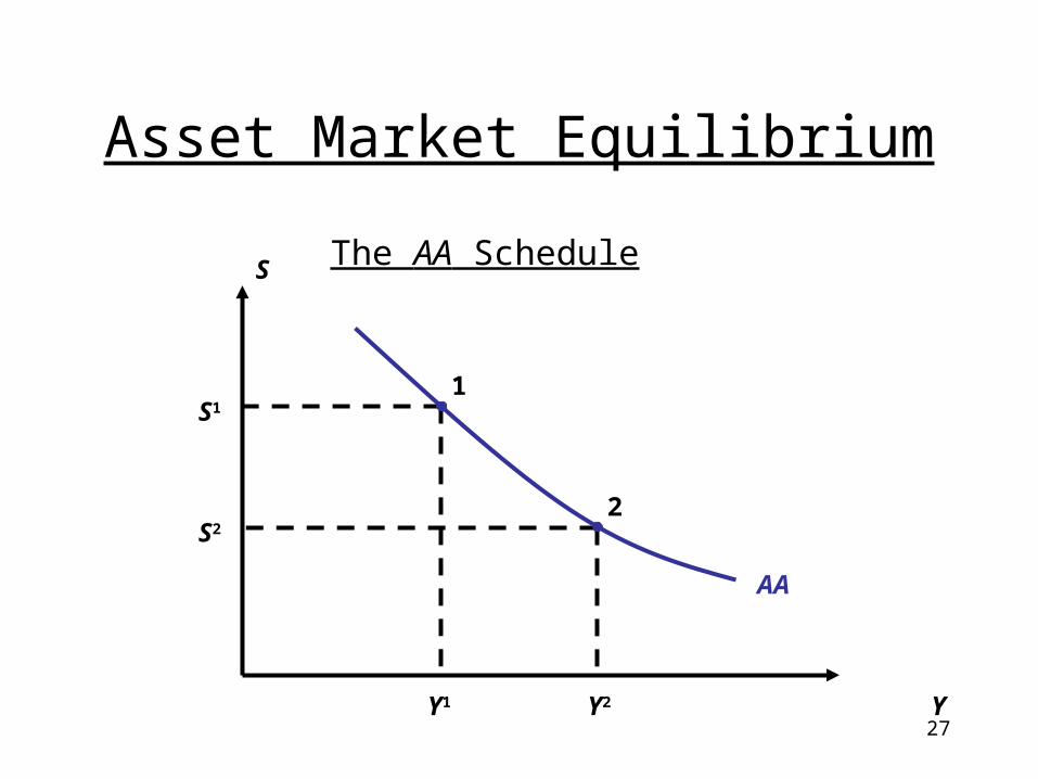
Asset Market Equilibrium
• Factors that affect the AA schedule– A change in the nominal exchange rate or of output is a
move along the AA schedule.
– An increase in the home stock of money or a reduction in home prices shifts the AA schedule to the right.
– An increase in foreign interest rate or the expected future exchange rate shifts the AA schedule to the right.
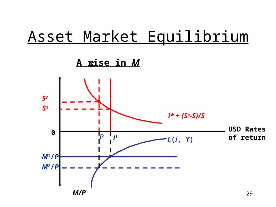
29
Asset Market Equilibrium
M/P
USD Rates of return
S
0
S2
S1
i* + (Se-S)/S
M1/P
M2/P
L(i, Y)i1i2
A rise in M
30
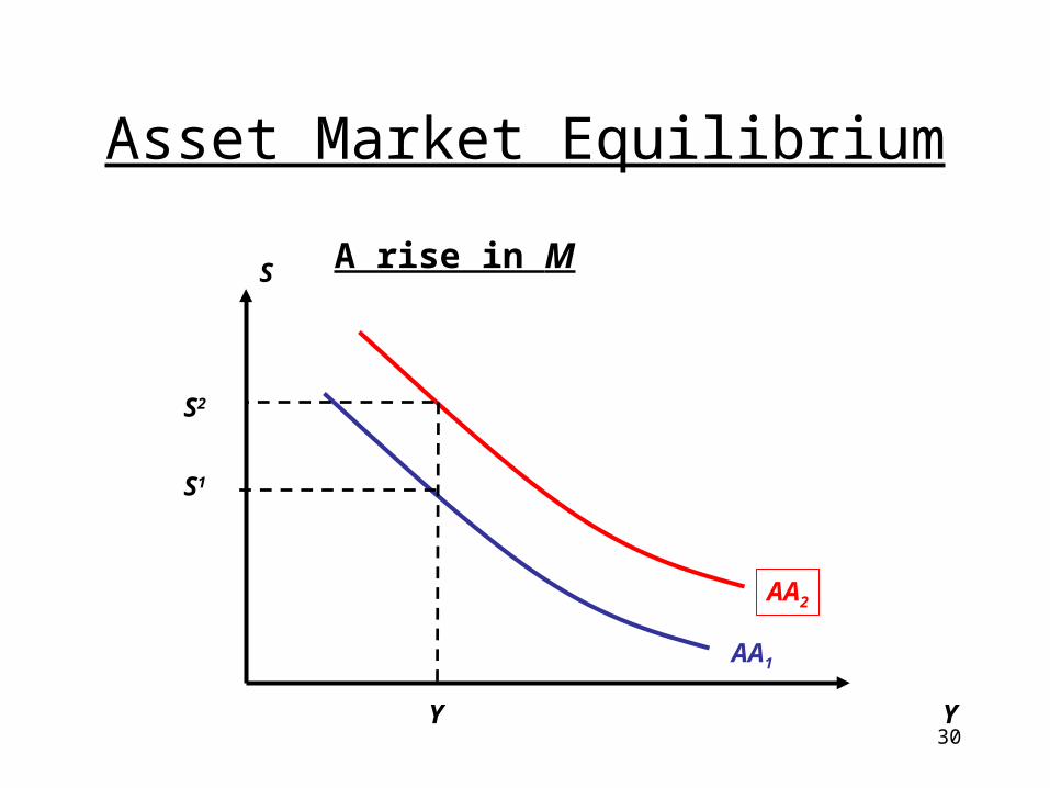
Asset Market Equilibrium
Y
S
AA2
A rise in M
AA1
S2
S1
Y
31
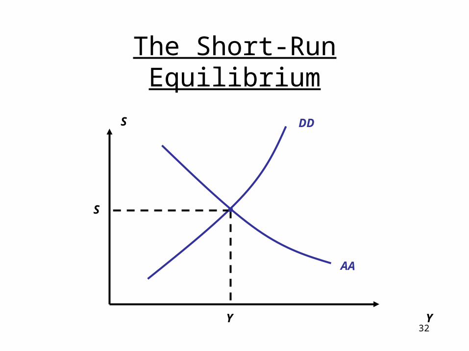
The Short-Run Equilibrium
• The short-run equilibrium brings equilibrium simultaneously to both the output and asset markets.
32
The Short-Run Equilibrium
Y
S DD
Y
S
AA
33
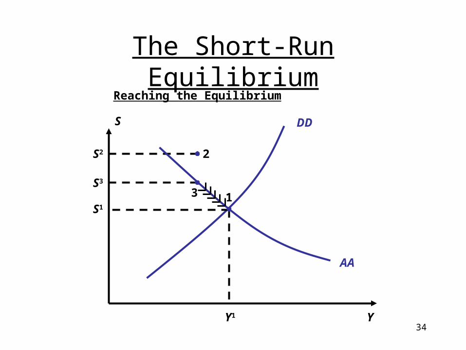
The Short-Run Equilibrium
• Reaching the short-run equilibrium.– The asset markets always reacts more rapidly.
• So, we first must move toward the AA schedule.
– The goods market is sticky (from sticky prices), and reacts more slowly.
34
The Short-Run Equilibrium
Y
S DD
Y1
S113
S3
2S2
AA
Reaching the Equilibrium
35
The Short-Run Equilibrium
• Reaching the short-run equilibrium– At point 2, the foreign exchange market is out of
equilibrium. S is so high that i> i*+(Se-S)/S.• There is an excess demand for home currency.
• So, S jumps down toward the AA schedule.
36
The Short-Run Equilibrium
– At point 3, the goods market is out of equilibrium. S is so high that Q = SP*/P is above its equilibrium level.
• This generates an excess demand for home goods.
• In response, the home economy ups Y and reduces S, to reduce the excess demand. So, S and Y move along the AA schedule slowly toward the DD schedule
37
Temporary Policy Changes
• Monetary policy– Policy instrument is the stock of money
supplied.
• Fiscal policy– Policy instrument is either taxes or government
expenditures.
38
Temporary Policy Changes
• Temporary Policy Changes– These policies have no effects on the expectations of
future exchange rates.– We expect these changes to be temporary, and to have
no effect on the long-run expected exchange rate.– So, we only worry about the short run, because we go
back to the initial equilibrium.
• For the following analysis, we assume that the different scenario involve no responses of foreign macroeconomic policies.
39
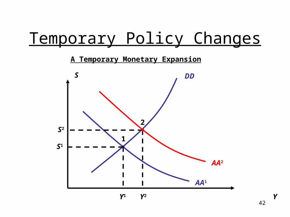
Temporary Policy Changes
• A Temporary Increase in Money Supply – The Money Market
• For fixed prices, the increase in the stock of money generates an excess supply of money. This reduces the home interest rate.
• The expansionary monetary policy also raises output, which increases money demand. The effect, however, is small. It slightly diminishes the reduction in the home interest rate.
40
Temporary Policy Changes
– The Foreign Exchange Market• The lower interest rate makes foreign investment
more attractive. This generate an excess demand of foreign currency. The result is that the foreign currency appreciates (or the home currency depreciates).
• This is a shift of the AA schedule to the right.
41
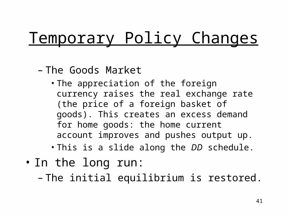
Temporary Policy Changes
– The Goods Market• The appreciation of the foreign currency raises the
real exchange rate (the price of a foreign basket of goods). This creates an excess demand for home goods: the home current account improves and pushes output up.
• This is a slide along the DD schedule.
• In the long run:– The initial equilibrium is restored.
42
Temporary Policy Changes
Y
S
AA1
DD
AA2
1S1
Y1 Y2
S22
A Temporary Monetary Expansion
43
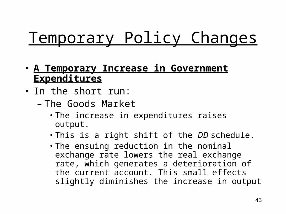
Temporary Policy Changes
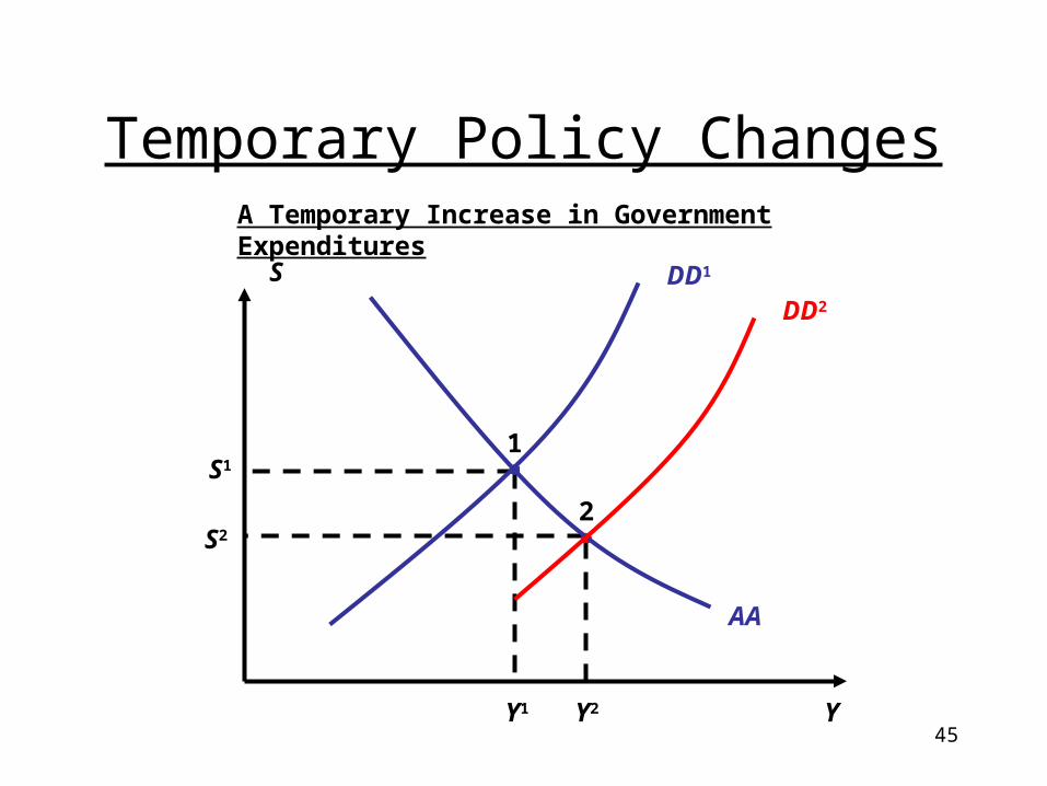
• A Temporary Increase in Government Expenditures
• In the short run:– The Goods Market
• The increase in expenditures raises output.• This is a right shift of the DD schedule.• The ensuing reduction in the nominal exchange rate
lowers the real exchange rate, which generates a deterioration of the current account. This small effects slightly diminishes the increase in output
44
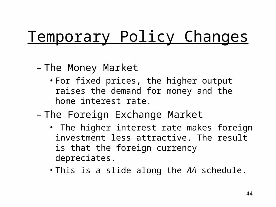
Temporary Policy Changes
– The Money Market• For fixed prices, the higher output raises the demand
for money and the home interest rate.
– The Foreign Exchange Market• The higher interest rate makes foreign investment
less attractive. The result is that the foreign currency depreciates.
• This is a slide along the AA schedule.
45
Temporary Policy Changes
Y
S
2
Y2
S2
Y1
S11
AA
DD2
DD1
A Temporary Increase in Government Expenditures
46
Temporary Policy Changes
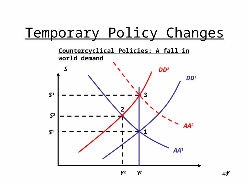
• The Business Cycle • Temporary fiscal and monetary policies can be
used to neutralize the effects of outside disturbances that create recessions.
47
Temporary Policy Changes
• For example, consider a temporary fall in world demand for home goods.– The fall in world demand creates a deterioration of the
home current account at current real exchange rate. This shifts the DD schedule to the left, which lowers output and raises the exchange rate.
• A temporary fiscal expansion (rise in G) would simply move the DD schedule back to its original position. This restores both output and the exchange rate.
• A temporary monetary expansion would shift the AA schedule to the right. This restores output, but raises further raises the exchange rate.
48
Temporary Policy Changes
Y
S
1S1
DD1
DD2
AA1
AA2
YfY2
S22
3S3
Countercyclical Policies: A fall in world demand
49
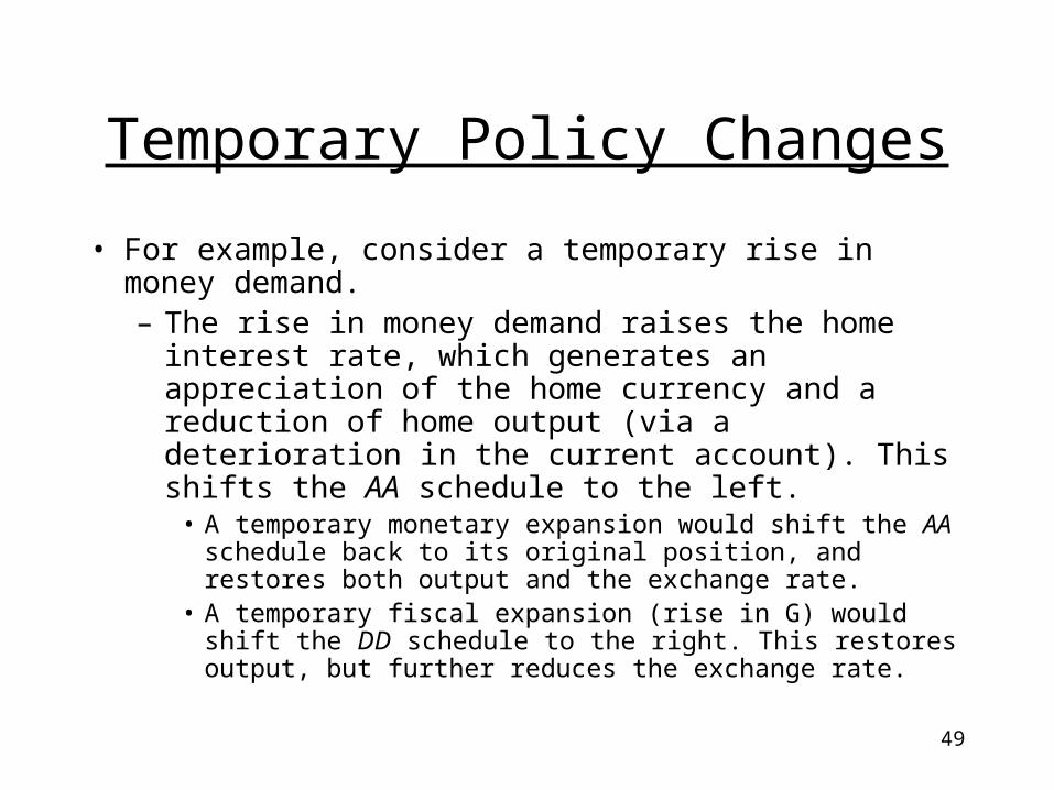
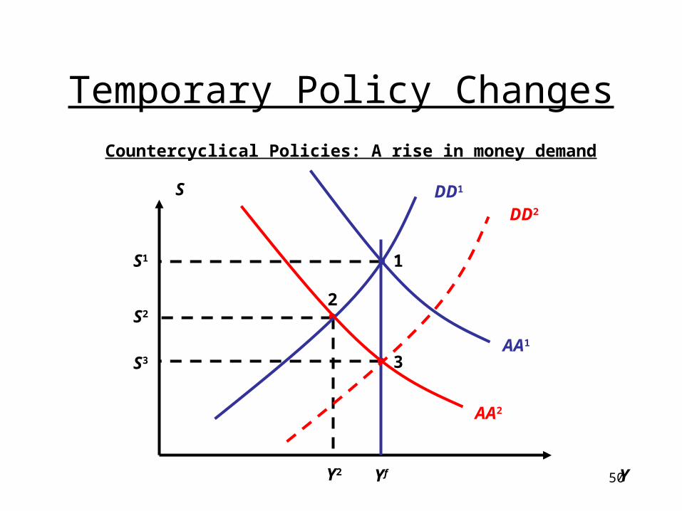
Temporary Policy Changes
• For example, consider a temporary rise in money demand.– The rise in money demand raises the home interest rate,
which generates an appreciation of the home currency and a reduction of home output (via a deterioration in the current account). This shifts the AA schedule to the left.
• A temporary monetary expansion would shift the AA schedule back to its original position, and restores both output and the exchange rate.
• A temporary fiscal expansion (rise in G) would shift the DD schedule to the right. This restores output, but further reduces the exchange rate.
50
Temporary Policy Changes
Y
S
3S3
Y2
S22
1S1
Yf
DD1
DD2
AA2
AA1
Countercyclical Policies: A rise in money demand
51
Permanent Policy Changes
• Unlike temporary changes, permanent policy changes potentially have long-run effects.
• These changes may affect the long-run exchange rate, and our expectations of the future exchange rate.
52
Permanent Policy Changes
• A Permanent Increase in the Money Supply• The Long Run: Perfect Price Flexibility
– The Money Market• The rise in M only raises P. Money is neutral in the
long run.
– The Foreign Exchange Market• The rise in P engineers a long-run depreciation of
the home currency (an increase in S).• This is a shift of the AA schedule to the right.
53
Permanent Policy Changes
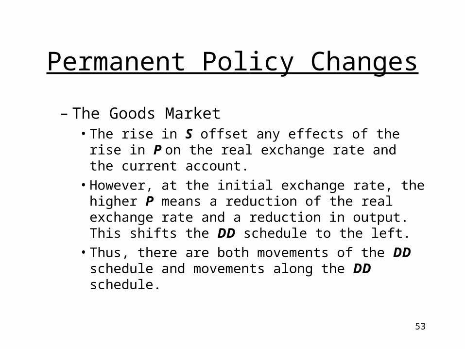
– The Goods Market• The rise in S offset any effects of the rise in P on the
real exchange rate and the current account.
• However, at the initial exchange rate, the higher P means a reduction of the real exchange rate and a reduction in output. This shifts the DD schedule to the left.
• Thus, there are both movements of the DD schedule and movements along the DD schedule.
54
Permanent Policy Changes
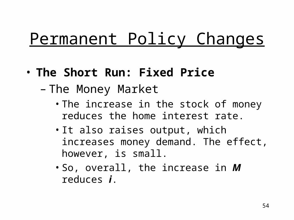
• The Short Run: Fixed Price– The Money Market
• The increase in the stock of money reduces the home interest rate.
• It also raises output, which increases money demand. The effect, however, is small.
• So, overall, the increase in M reduces i.
55
Permanent Policy Changes
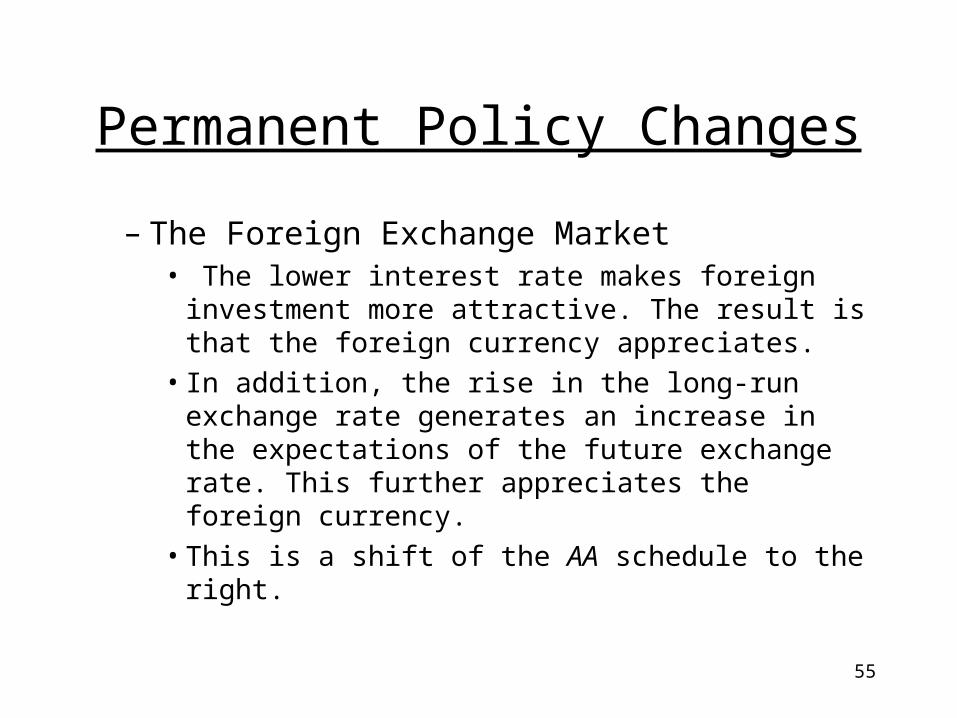
– The Foreign Exchange Market• The lower interest rate makes foreign investment
more attractive. The result is that the foreign currency appreciates.
• In addition, the rise in the long-run exchange rate generates an increase in the expectations of the future exchange rate. This further appreciates the foreign currency.
• This is a shift of the AA schedule to the right.
56
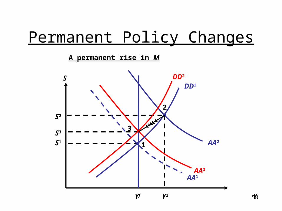
Permanent Policy Changes
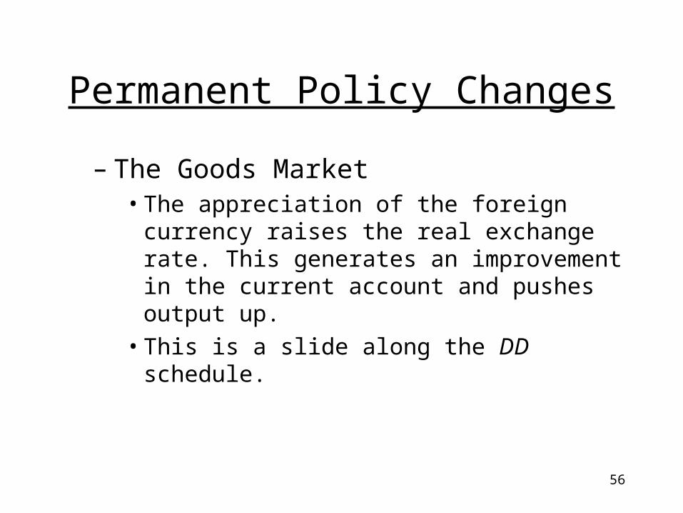
– The Goods Market• The appreciation of the foreign currency raises the
real exchange rate. This generates an improvement in the current account and pushes output up.
• This is a slide along the DD schedule.
57
Permanent Policy Changes
• The adjustment: the short run to the long run– The Money Market:
• As prices rise, the interest rate and output are slowly restored to the initial level.
– The Foreign Exchange Market:• The rising home interest rate generates a
depreciation of the foreign currency.
– The Goods Market:
58
Permanent Policy Changes
Y
S
Y2
S2
2
3S3
S11
Yf
AA1AA3
AA2
DD2
DD1
A permanent rise in M
59
Permanent Policy Changes
• A Permanent Rise in Government Exp.• The Long Run: Perfect Price Flexibility
– The Goods Market• The increase in expenditures raises output.
• This raises the demand for home goods, and lowers the price of foreign goods.
• The reduction in the real exchange rate lowers the nominal exchange rate.
60
Permanent Policy Changes
– The Money Market• No changes in the long run.
– The Foreign Exchange Market• The expected future exchange rate drops, lowering
the foreign return schedule.
61
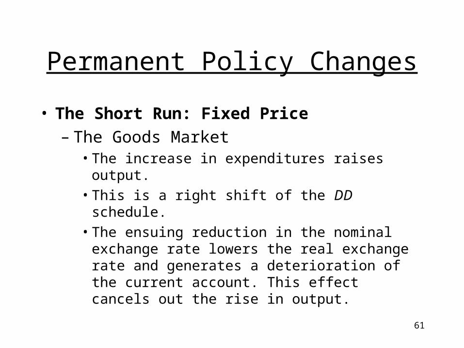
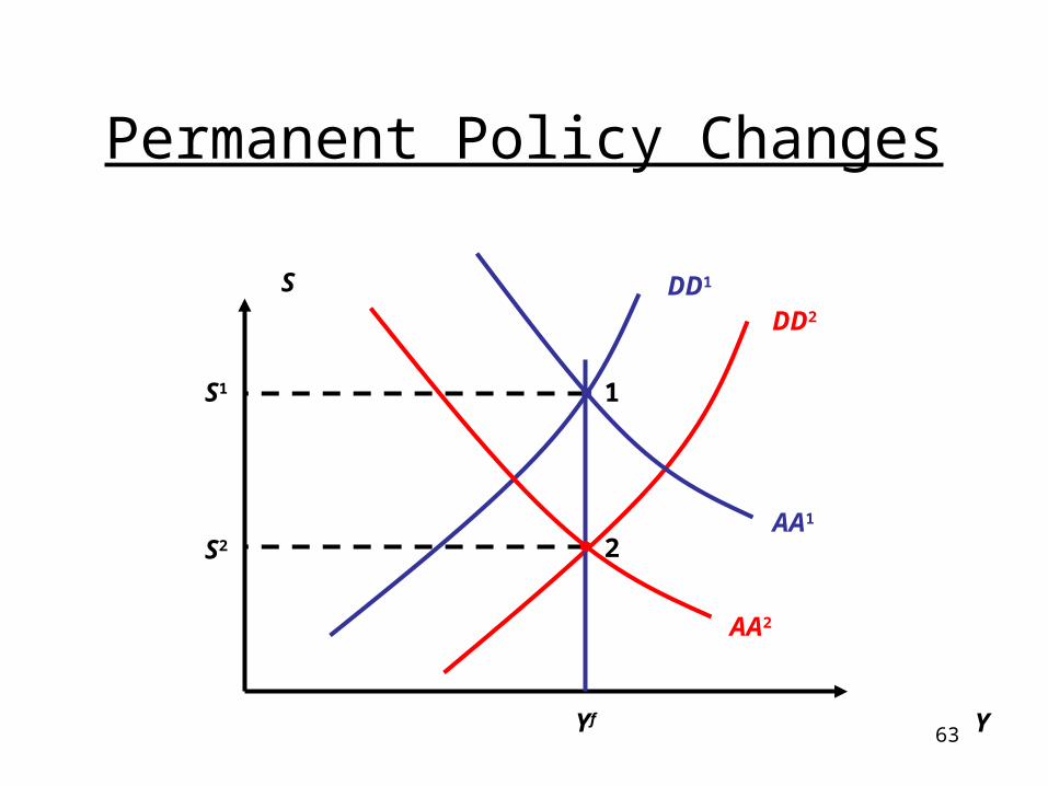
Permanent Policy Changes
• The Short Run: Fixed Price– The Goods Market
• The increase in expenditures raises output.
• This is a right shift of the DD schedule.
• The ensuing reduction in the nominal exchange rate lowers the real exchange rate and generates a deterioration of the current account. This effect cancels out the rise in output.
62
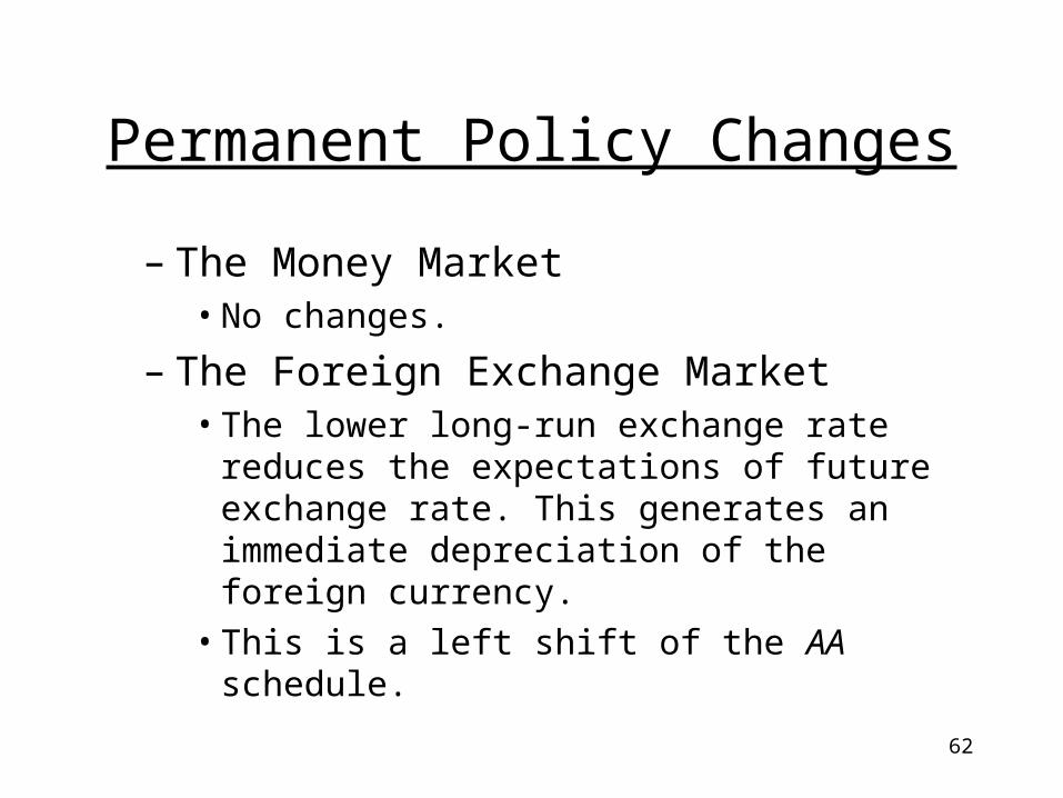
Permanent Policy Changes
– The Money Market• No changes.
– The Foreign Exchange Market• The lower long-run exchange rate reduces the
expectations of future exchange rate. This generates an immediate depreciation of the foreign currency.
• This is a left shift of the AA schedule.
63
Permanent Policy Changes
Y
S DD1
DD2
AA2
AA1
Yf
2S2
1S1
64
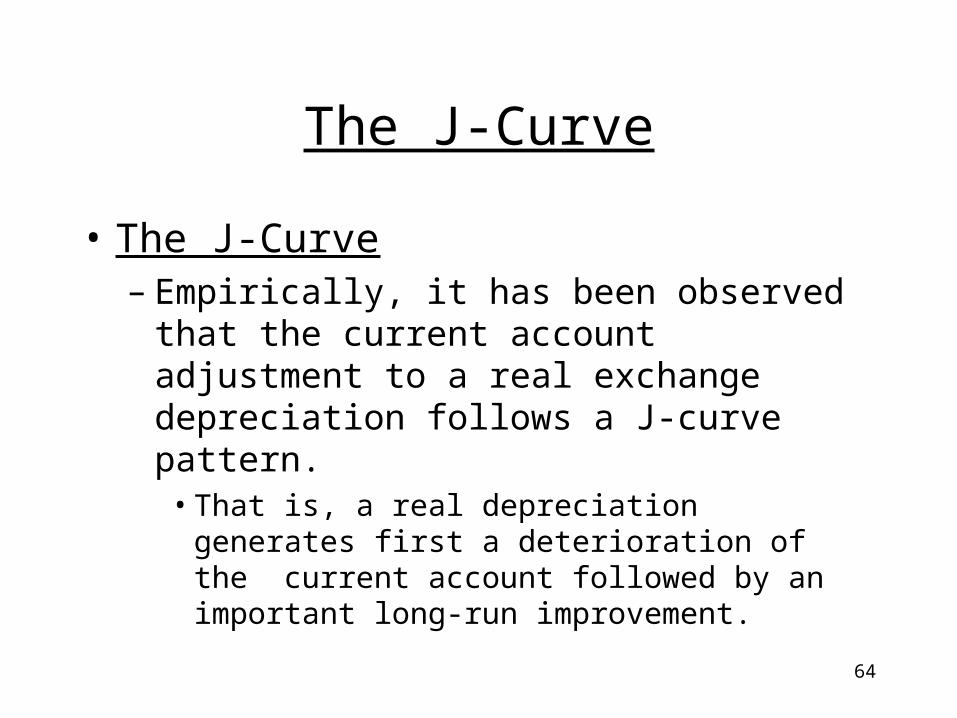
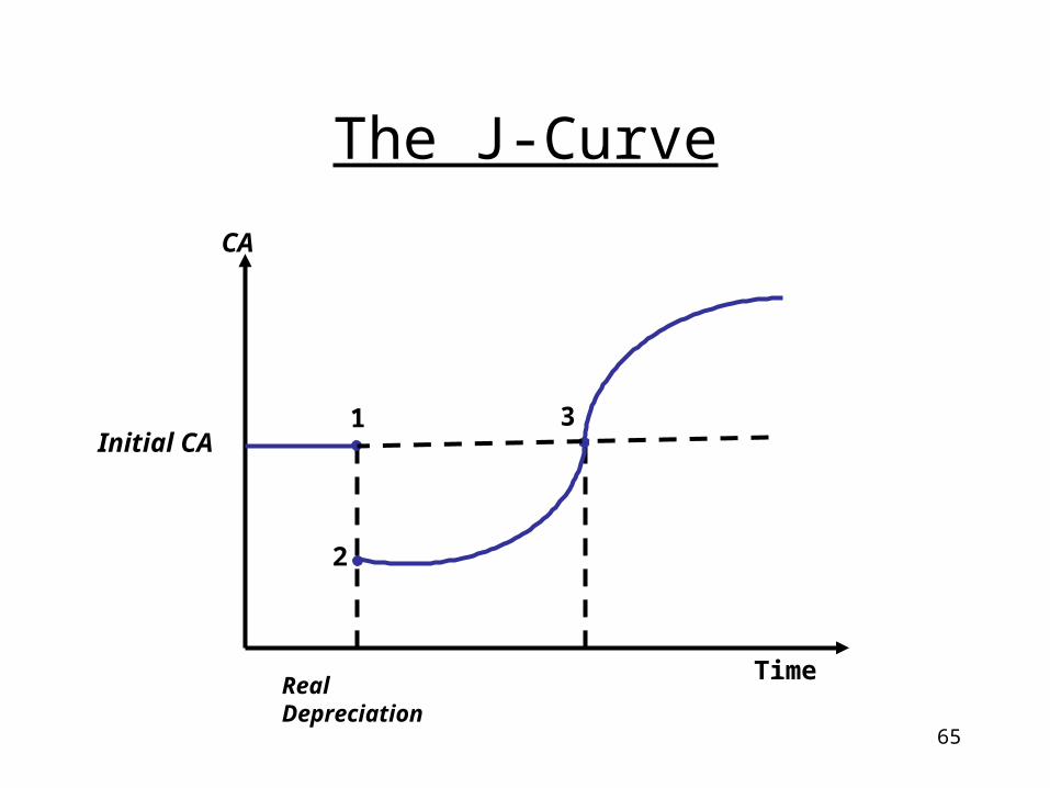
The J-Curve
• The J-Curve– Empirically, it has been observed that the
current account adjustment to a real exchange depreciation follows a J-curve pattern.
• That is, a real depreciation generates first a deterioration of the current account followed by an important long-run improvement.
65
The J-Curve
Time
CA
2
31Initial CA
RealDepreciation
66
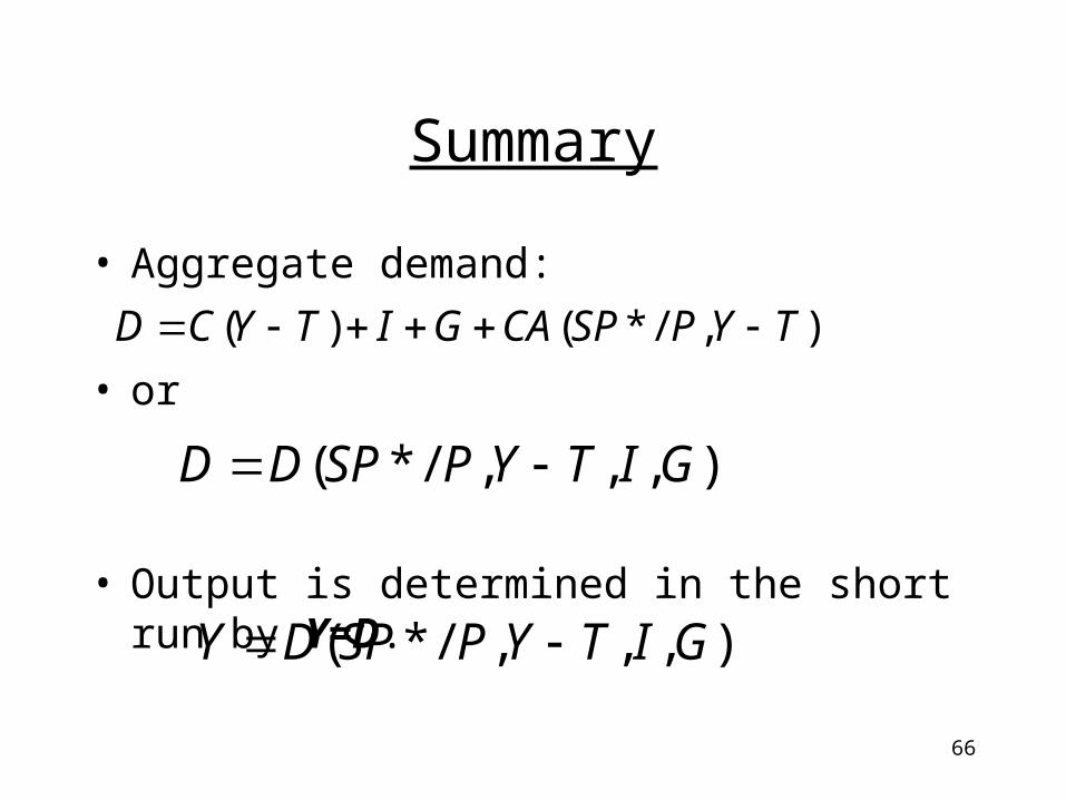
Summary
• Aggregate demand:
• or
• Output is determined in the short run by Y=D.
),/*()( TYPSPCAGITYCD
),,,/*( GITYPSPDD
),,,/*( GITYPSPDY
67
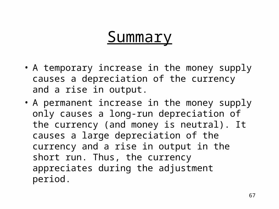
Summary
• A temporary increase in the money supply causes a depreciation of the currency and a rise in output.
• A permanent increase in the money supply only causes a long-run depreciation of the currency (and money is neutral). It causes a large depreciation of the currency and a rise in output in the short run. Thus, the currency appreciates during the adjustment period.
68
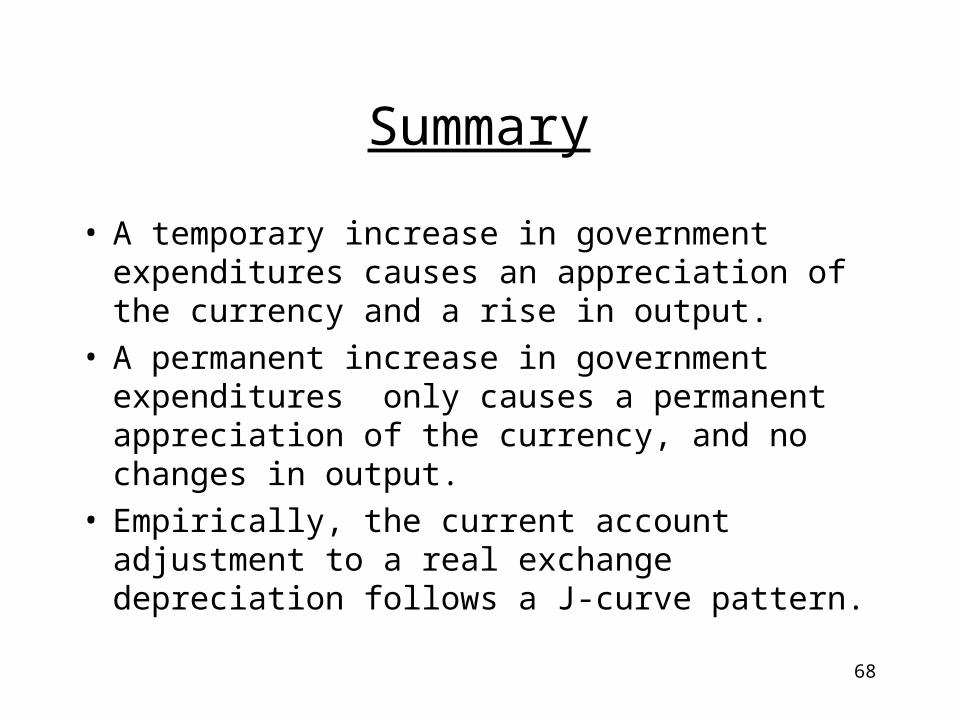
Summary
• A temporary increase in government expenditures causes an appreciation of the currency and a rise in output.
• A permanent increase in government expenditures only causes a permanent appreciation of the currency, and no changes in output.
• Empirically, the current account adjustment to a real exchange depreciation follows a J-curve pattern.


![[ADVANCED ECONOMIC ANALYSIS]€¦ · M.A. Economics, Semester-II Advanced Economic Analysis-II Unit Syllabus UNIT-1 –Perfect competition short run and long run equilibrium of the](https://img.pdfslide.net/doc/110x75/5fcb159187ee5e6f4b08b84d/advanced-economic-analysis-ma-economics-semester-ii-advanced-economic-analysis-ii.jpg)