1

SIMS 290-2: Applied Natural Language Processing

Preslav NakovSept 29, 2004 

 

2

Today

Feature selectionTF.IDF Term WeightingTerm Normalization

3

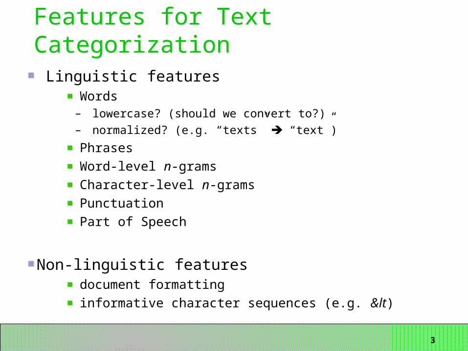
Features for Text Categorization

Linguistic features Words– lowercase? (should we convert to?)– normalized? (e.g. “texts” “text”)

Phrases Word-level n-grams Character-level n-grams Punctuation Part of Speech

Non-linguistic features

document formatting informative character sequences (e.g. &lt)

4

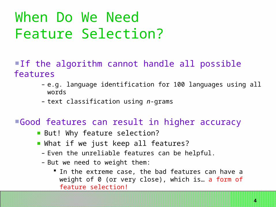
If the algorithm cannot handle all possible features– e.g. language identification for 100 languages using all words– text classification using n-grams

Good features can result in higher accuracy But! Why feature selection? What if we just keep all features?– Even the unreliable features can be helpful.– But we need to weight them:

In the extreme case, the bad features can have a weight of 0 (or very close), which is… a form of feature selection!

When Do We NeedFeature Selection?

5

Why Feature Selection?

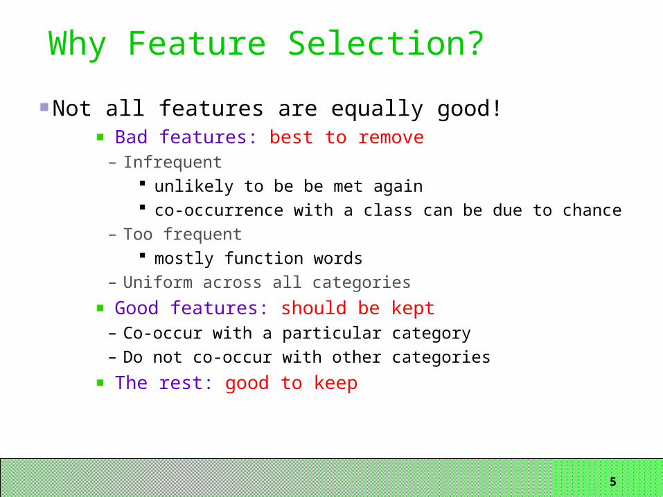
Not all features are equally good! Bad features: best to remove– Infrequent

unlikely to be be met again co-occurrence with a class can be due to chance

– Too frequent mostly function words

– Uniform across all categories

Good features: should be kept– Co-occur with a particular category– Do not co-occur with other categories

The rest: good to keep

6

Types Of Feature Selection?

Feature selection reduces the number of features Usually:

Eliminating features Weighting features Normalizing features

Sometimes by transforming parameters e.g. Latent Semantic Indexing using Singular Value

Decomposition

Method may depend on problem type For classification and filtering, may use information from example documents to guide selection

7

Feature Selection

Task independent methodsDocument Frequency (DF)Term Strength (TS)

Task-dependent methodsInformation Gain (IG)Mutual Information (MI)2 statistic (CHI)

Empirically compared by Yang & Pedersen (1997)

8

Pedersen & Yang Experiments

Compared feature selection methods for text categorization

5 feature selection methods:– DF, MI, CHI, (IG, TS)– Features were just words

2 classifiers: – kNN: k-Nearest Neighbor (to be covered next week)– LLSF: Linear Least Squares Fit

2 data collections:– Reuters-22173– OHSUMED: subset of MEDLINE (1990&1991 used)

9

DF: number of documents a term appears in

Based on Zipf’s LawRemove the rare terms: (met 1-2 times)

Non-informative Unreliable – can be just noise Not influential in the final decision Unlikely to appear in new documents

Plus Easy to compute Task independent: do not need to know the classes

Minus Ad hoc criterion Rare terms can be good discriminators (e.g., in IR)

Document Frequency (DF)

What about the frequent terms?

What is a “rare” term?

10

Examples of Frequent Words:Most Frequent Words in Brown Corpus

11

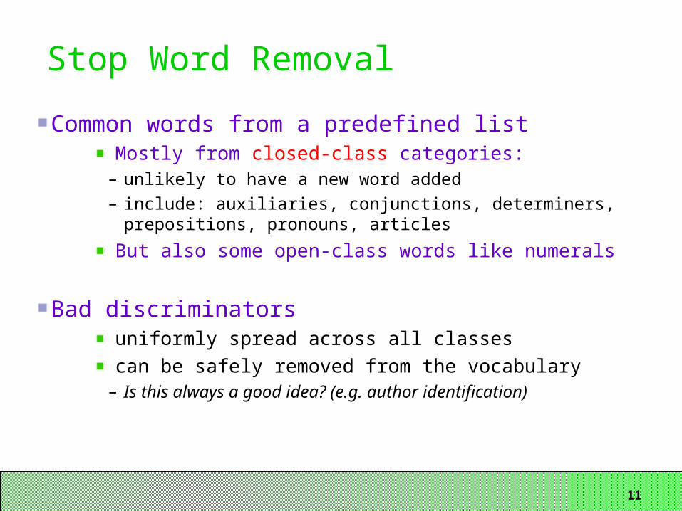
Common words from a predefined list Mostly from closed-class categories: – unlikely to have a new word added– include: auxiliaries, conjunctions, determiners, prepositions,

pronouns, articles

But also some open-class words like numerals

Bad discriminators uniformly spread across all classes can be safely removed from the vocabulary– Is this always a good idea? (e.g. author identification)

Stop Word Removal

12

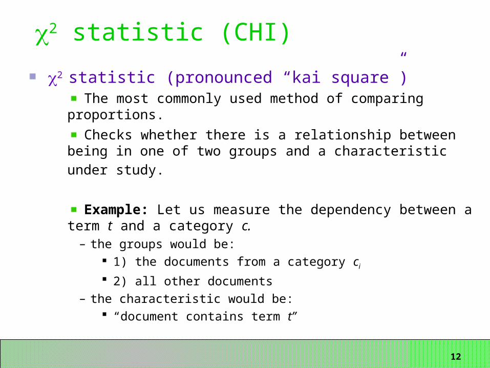
2 statistic (pronounced “kai square”) The most commonly used method of comparing

proportions.

Checks whether there is a relationship between being in one of two groups and a characteristic under study.

Example: Let us measure the dependency between a term t and a category c.

– the groups would be: 1) the documents from a category ci 2) all other documents

– the characteristic would be: “document contains term t”

2 statistic (CHI)

13

Is “jaguar” a good predictor for the “auto” class?

We want to compare: the observed distribution above; and null hypothesis: that jaguar and auto are independent

2 statistic (CHI)

Term = jaguar Term jaguar

Class = auto 2 500

Class auto 3 9500

14

Under the null hypothesis: (jaguar and auto – independent): How many co-occurrences of jaguar and auto do we expect?

We would have: Pr(j,a) = Pr(j) Pr(a)

So, there would be: N Pr(j,a), i.e. N Pr(j) Pr(a)

Pr(j) = (2+3)/N; Pr(a) = (2+500)/N; N=2+3+500+9500

Which is: N(5/N)(502/N)=2510/N=2510/10005 0.25

2 statistic (CHI)

Term = jaguar Term jaguar

Class = auto 2 500

Class auto 3 9500

15

Under the null hypothesis: (jaguar and auto – independent): How many co-occurrences of jaguar and auto do we expect?

We would have: Pr(j,a) = Pr(j) Pr(a)

So, there would be: N Pr(j,a), i.e. N Pr(j) Pr(a)

Pr(j) = (2+3)/N; Pr(a) = (2+500)/N; N=2+3+500+9500

Which is: N(5/N)(502/N)=2510/N=2510/10005 0.25

2 statistic (CHI)

Term = jaguar Term jaguar

Class = auto 2 (0.25) 500

Class auto 3 9500

expected: fe

observed: fo

16

Under the null hypothesis: (jaguar and auto – independent): How many co-occurrences of jaguar and auto do we expect?

We would have: Pr(j,a) = Pr(j) Pr(a)

So, there would be: N Pr(j,a), i.e. N Pr(j) Pr(a)

Pr(j) = (2+3)/N; Pr(a) = (2+500)/N; N=2+3+500+9500

Which is: N(5/N)(502/N)=2510/N=2510/10005 0.25

2 statistic (CHI)

Term = jaguar Term jaguar

Class = auto 2 (0.25) 500 (502)

Class auto 3 (4.75) 9500 (9498)

expected: fe

observed: fo

17

2 is interested in (fo – fe)2/fe summed over all table entries:

The null hypothesis is rejected with confidence .999, since 12.9 > 10.83 (the value for .999 confidence).

2 statistic (CHI)

)001.(9.129498/)94989500(502/)502500(

75.4/)75.43(25./)25.2(/)(),(22

2222

p

EEOaj

Term = jaguar Term jaguar

Class = auto 2 (0.25) 500 (502)

Class auto 3 (4.75) 9500 (9498)

expected: fe

observed: fo

18

There is a simpler formula for 2:

2 statistic (CHI)

N = A + B + C + D

A = #(t,c) C = #(¬t,c)

B = #(t,¬c) D = #(¬t, ¬c)

19

How to use 2 for multiple categories?

Compute 2 for each category and then combine: we can require to discriminate well across all categories,

then we need to take the expected value of 2:

or to discriminate well for a single category, then we take the maximum:

2 statistic (CHI)

20

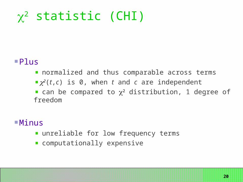
Plus normalized and thus comparable across terms 2(t,c) is 0, when t and c are independent can be compared to 2 distribution, 1 degree of freedom

Minus unreliable for low frequency terms computationally expensive

2 statistic (CHI)

21

Information Gain

A measure of importance of the feature for predicting the presence of the class.Defined as:

The number of “bits of information” gained by knowing the term is present or absentBased on Information Theory

– We won’t go into this in detail here.

Plus:sound information theory justification

Minus:computationally expensive

22

Information Gain (IG)

IG: number of bits of information gained by knowing the term is present or absent

t is the term being scored, ci is a class variable

entropy: H(c)

specificconditionalentropy H(c|t)

specificconditionalentropy H(c|¬t)

23

The probability of seeing x followed by y vs. the probably of seeing x anywhere times the probability of seeing y anywhere.

log ( P(x,y) / P(x)P(y) )

Mutual Information (MI)

24

Approximation:

Mutual Information (MI)

A = #(t,c) C = #(¬t,c)

B = #(t,¬c)

D = #(¬t, ¬c)

rare terms scored higher

does not useterm absence

25

Compute MI for each category and then combine If we want to discriminate well across all categories, then

we need to take the expected value of MI:

To discriminate well for a single category, then we take the maximum:

Using Mutual Information

26

Mutual Information

PlusI(t,c) is 0, when t and c are independentSound information-theoretic interpretation

MinusSmall numbers produce unreliable resultsComputationally expensiveDoes not use term absence

27

Mutual information

Term strength

28

DF, IG and CHI are good and strongly correlated thus using DF is good, cheap and task independent can be used when IG and CHI are too expensive

MI is bad favors rare terms (which are typically bad)

MI vs. IG

Comparison: DF,TS,IG,CHI,MI

mutualinformation

informationgain

29

Term Weighting

In the study just shown, terms were (mainly) treated as binary features

If a term occurred in a document, it was assigned 1Else 0

Often it us useful to weight the selected featuresStandard technique: tf.idf

30

TF: term frequency definition: TF = tij – frequency of term i in document j

purpose: makes the frequent words for the document more important

IDF: inverted document frequency definition: IDF = log(N/ni)

– ni : number of documents containing term i

– N : total number of documents

purpose: makes rare words across documents more important

TF.IDF definition: tij log(N/ni)

TF.IDF Term Weighting

31

Term Normalization

Combine different words into a single representation

Stemming/morphological analysis– bought, buy, buys -> buy

General word categories – $23.45, 5.30 Yen -> MONEY– 1984, 10,000 -> DATE, NUM– PERSON– ORGANIZATION

(Covered in Information Extraction segment)Generalize with lexical hierarchies

– WordNet, MeSH (Covered later in the semester)

32

Purpose: conflate morphological variants of a word to a single index term

Stemming: normalize to a pseudoword– e.g. “more” and “morals” become “mor” (Porter stemmer)

Lemmatization: convert to the root form– e.g. “more” and “morals” become “more” and “moral”

Plus:vocabulary size reductiondata sparseness reduction

Minus:loses important features (even to_lowercase() can be bad!)questionable utility (maybe just “-s”, “-ing” and “-ed”?)

Stemming & Lemmatization

33

1. Feature selectioninfrequent term removal

infrequent across the whole collection (i.e. DF)met in a single document

most frequent term removal (i.e. stop words)

2. Normalization:1. Stemming. (often) 2. Word classes (sometimes)

3. Feature weighting: TF.IDF or IDF4. Dimensionality reduction. (occasionally)

What Do People Do In Practice?

34

Summary

Feature selectionTask independent methods: DF, TSTask dependent: IG, MI, 2 statistic

Term weightingIDFTF.IDF

Term normalization

35

Feature Selection Yang Y., J. Pedersen. A comparative study on feature

selection in text categorization. In J. D. H. Fisher, editor, The Fourteenth International Conference on Machine Learning (ICML'97), pages 412-420. Morgan Kaufmann, 1997.

Term Weighting Salton G., C. Buckley, Term-weighting approaches in

automatic text retrieval, Information Processing and Management: an International Journal, v.24 n.5, p.513-523, 1988.

Salton, G. 1989. Automatic text processing. Chapter 9.

References