Embed Size (px)
Citation preview

1
Speech Parametrisation
• Compact encoding of information in speech
• Accentuates important info– Attempts to eliminate irrelevant information
• Accentuates stable info– Attempts to eliminate factors which tend to
vary most across utterances (and speakers)

2
40ms
20ms
Frames
• Parameterise on a frame-by-frame basis
• Choose frame length, over which speech remains reasonably stationary
• Overlap frames e.g. 40ms frames, 10ms frame shift

3
Crude Parametrisation• Time domain• Use short-term energy (STE)• Sequentially segment the speech signal into
frames• Calculate STE for each frame• STE:
frame
nST sE 2
• n refers to the nth sample

4
0 0.1 0.2 0.3 0.4 0.5 0.6 0.7 0.8-1
0
1
yes
0 0.1 0.2 0.3 0.4 0.5 0.6 0.7 0.8-1
0
1
no
0 2 4 6 8 10 12 14 16 180
100
200
STE yesSTE no

5
Why not use waveform samples?
• How many samples in a frame?– The more numbers the more computation
• How can we measure similarity?
• Use what we know about speech…– Spectrum!

6
Crude Parametrisation
• Frequency related
• Use zero-crossing rate (ZCR)
• Calculate ZCR for each frame:
frame
nnZCR
ssM
2
)(sign)(sign 1
• where:
01
01)(sign
x-
xx

7
0 0.1 0.2 0.3 0.4 0.5 0.6 0.7 0.8-1
0
1
yes
0 0.1 0.2 0.3 0.4 0.5 0.6 0.7 0.8-1
0
1
no
0 2 4 6 8 10 12 14 16 180
200
400
600
ZCR yesZCR no

8
Multidimensionality
• We can combine multiple features into a feature vector
• Let’s combine STE and ZCR and measure the magnitude of each feature vector
• More complex multidimensional feature vectors are generally used in ASR
STE
ZCR
2-dimensionalFeature Vector

9
0 0.1 0.2 0.3 0.4 0.5 0.6 0.7 0.8-1
0
1
yes
0 0.1 0.2 0.3 0.4 0.5 0.6 0.7 0.8-1
0
1
no
0 2 4 6 8 10 12 14 16 180
0.5
1
1.5
ZC_E yesZC_E no

10
Parametrisation: Sophistication• We need something more
representative of the information in the speech less prone to variation
• The spectral slices we have been viewing to date in Praat are actually LPC (Linear Predictive Coding) spectra
• LPC attempts to remove the effects of phonation– Leaves us with correlate of VT
configuration

11
Spectral Feature Extraction
• Extract compact set of spectral parameters (features) for each frame
• Frames usually overlapping

12
DFT spectra vs LPC spectra
• DFT (Discrete Fourier Transform)– Technique ubiquitous in DSP for spectral analysis– fft function in MATLAB
• demo > Numerics> Fast Fourier Transform
– Demo function dftdemo_sinusoid_sig
• LPC – Mathematical encoding of signals– Based on modelling speech as a series of sums of
exponentially decaying sinusoids– Source-filter decomposition– Typical example of how spectral information can be
compressed

13
Preprocessing Speech for Spectral Estimation
1. Choose frequency resolution– Time/Frequency trade off– Parametrisation frame length
2. Pre-emphasise– Flattens spectrum which reduces spectral
dynamic range which eases estimation
3. Apply window function in time domain– Tapers frame boundary values to zero– Gives better picture of spectrum

14
DFT Spectrum /u/
0 1000 2000 3000 4000 5000 6000-30
-20
-10
0
10
20
30
40

15
Frame Length:{5,40,200}ms
2 2.05 2.1 2.15 2.2 2.25
x 104
-0.6
-0.4
-0.2
0
0.2
0.4
0.6
0.8

16
Freq. Resolution for {5,40,200}ms
0 1000 2000 3000 4000 5000 6000-30
-20
-10
0
10
20
30
40
50

17
Preemphasis: using diff
2 2.01 2.02 2.03 2.04 2.05
x 104
-0.6
-0.4
-0.2
0
0.2
0.4
0.6
0.8

18
Preemphasis
0 1000 2000 3000 4000 5000 6000-40
-30
-20
-10
0
10
20
30
40

19
Windowing: using hamming
2 2.01 2.02 2.03 2.04 2.05
x 104
-0.2
0
0.2
0.4
0.6
0.8
1
1.2Hamming Window

20
Windowing: Spectral Effect
0 1000 2000 3000 4000 5000 6000-60
-50
-40
-30
-20
-10
0
10
20

21
LPC Spectrum: using lpc
0 1000 2000 3000 4000 5000 6000-60
-50
-40
-30
-20
-10
0
10
20LP Order = 14
22
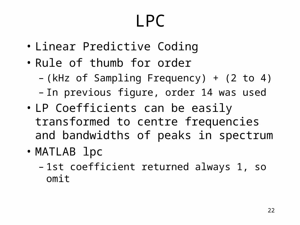
LPC
• Linear Predictive Coding
• Rule of thumb for order– (kHz of Sampling Frequency) + (2 to 4)– In previous figure, order 14 was used
• LP Coefficients can be easily transformed to centre frequencies and bandwidths of peaks in spectrum
• MATLAB lpc– 1st coefficient returned always 1, so omit

23
Cepstrally Smoothed Spectrum
0 1000 2000 3000 4000 5000 6000-60
-50
-40
-30
-20
-10
0
10
2025 Cepstral Coefficients

24
MFCCs
• Mel Frequency Cepstral Coefficients– Encodes/compresses spectral info in
approx. 12 coefficients– Weights areas of perceptual importance
more heavily– Will use them in HTK– Other parameterisations possible