1st order linear differential equation:

P, Q – continuous.)()( xQyxP

dx

dy

Algorithm:

Find I(x), s.t.

)()())(())(()( xQxIyxIyxPyxI

)()()( xPxIdx

dIyIyIyIyPIyI

by solving differential equation for I(x):

dxxP

exI)(

)(

CdxxQxIyxIxQxIyxI )()()()()())((

then integrate both sides of the equation:

Simplify the expression, if possible.

2nd order linear differential equation:

P, Q, R, G – continuous.

)()()()(2

2

xGyxRdx

dyxQ

dx

ydxP

If G(x)0 equation is homogeneous, otherwise – nonhomogeneous.

2nd order linear homogeneous differential equation –

0)()()(2

2

yxRdx

dyxQ

dx

ydxP

1). If y1 and y2 are solutions, then y=c1y1+c2y2 (linear combination) is also a solution.

2). If y1 and y2 are linearly independent solutions and P0, then the general solution is y=c1y1+c2y2.

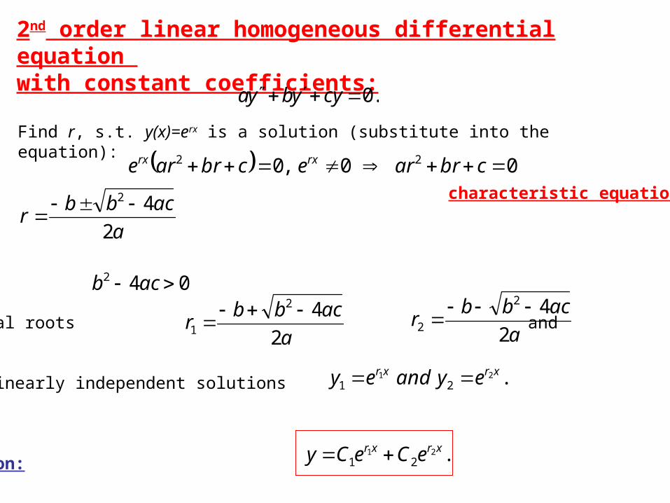
2nd order linear homogeneous differential equation with constant coefficients:

.0 cyybya

Find r, s.t. y(x)=erx is a solution (substitute into the equation):

00,0 22 cbrarecbrare rxrx

characteristic equation

a

acbbr

2

42

Case I.

Two unequal real roots and

Therefore, 2 linearly independent solutions

General solution:

042 acb

a

acbbr

2

42

1

a

acbbr

2

42

2

.2121

xrxr eyandey

.2121

xrxr eCeCy

Case II.

One real root

Two linearly independent solutions are

General solution:

042 acb

a

brrr

221

.21rxrx xeyandey

.21rxrx xeCeCy

Case III.

Two complex roots

Two linearly independent solutions

General solution:

.1,44

)04..(04

22

22

iwherebaciacb

baceiacb

a

bac

a

bwhere

irandir

2

4,

2

,

2

21

.sincos 21 xCxCey x

.sincos 21 xeyandxey xx

Problems

2. Volumes by washer method (Sec. 6.2) and by cylindrical shells method (Sec 6.3):

Find the volume of the solid obtained by rotating the region bounded by

about x=-1.

2xyandxy

1. Area between curves:

Set up the area between the following curves:

a)

b)

Sec. 6.1 5-26

29,12 xyxy 22,1 yxyx

3. Arclength (Sec. 8.1):

Find the arclength of the curve .3

0),ln(cos

xxy

4. Approximate integration (Sec. 7.7). Rn, Ln, Mn, Tn, Sn, formulae and error approximation:

How large should we take n for Trapezoid / Midpoint / Simpson’s Rules in order to

guarantee that the error of each method for would be within 0.001?

Write down the expressions for R5, L5, M5, T5, S5.

2

1 x

dx

5. L’Hospital Rule (Sec. 4.4):

Find Justify every time you apply L’Hospital rule!.)(ln

lim2

x

xx

6. Improper integral (Sec. 7.8): type I, type II.

7. Differential equations:

1st order separable equation (Sec. 9.3):

1st order linear equation (Sec. 9.6):

2nd order linear equation (Sec. 17.1):

Initial Value Problem and Boundary Value Problem.

8. Modeling: mixing problem, fish growth problem, population growth:

The population of the world was 5.28 billion in 1990 and 6.07 billion in 2000. Assuming

that the population growth rate is proportional to the size of population, formulate and

solve the corresponding differential equation. Predict world population in 2020. When will

the world population exceed 10 billion?

9. Recall: graphs and derivatives of elementary functions, integration techniques.

.2 yyx

.12 xyyx

.0136,02,03 yyyyyyyyy

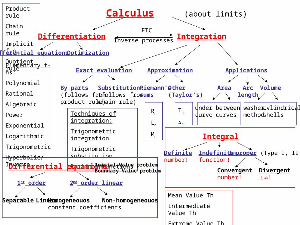
Calculus (about limits)

Differentiation IntegrationInverse processes

FTC

Product rule

Chain rule

Implicit f-n

Quotient rule

Exact evaluation Approximation Applications

By parts(follows from product rule)

Substitution(follows from chain rule)

Techniques of integration:

Trigonometric integration

Trigonometric substitution

Rational functions

Riemann’s sums

Other(Taylor’s)

Rn

Ln

Mn

Tn

Sn

Area VolumeArclength

under curve

betweencurves

washermethod

cylindricalshells

Integral

Definitenumber!

Indefinitefunction!

Improper (Type I, II)

Convergentnumber!

Divergent!

OptimizationDifferential equations

Differential equations

1st order 2nd order linear

Separable Linear Homogeneouosconstant coefficients

Non-homogeneouos

Elementary f-ns:

Polynomial

Rational

Algebraic

Power

Exponential

Logarithmic

Trigonometric

Hyperbolic/Inverse

Mean Value Th

Intermediate Value Th

Extreme Value Th

Initial Value problemBoundary Value problem