1 STOCHASTIC PROCESSES: LEARNING THE ...janroman.dhis.org/finance/Books Notes Thesises etc/Stoc...Mathematics, Finance and General Insurance. We hope that this paper will encourage

1

STOCHASTIC PROCESSES: LEARNING THE LANGUAGE

BY A. J. G. CAIRNS, D. C. M. DICKSON, A. S. MACDONALD,H. R. WATERS AND M. WILLDER

ABSTRACT

Stochastic processes are becoming more important to actuaries: they underlie much of modernfinance, mortality analysis and general insurance; and they are reappearing in the actuarial syllabus. Theyare immensely useful, not because they lead to more advanced mathematics (though they can do that) butbecause they form the common language of workers in many areas that overlap actuarial science. It isprecisely because most financial and insurance risks involve events unfolding as time passes that modelsbased on processes turn out to be most natural. This paper is an introduction to the language of stochasticprocesses. We do not give rigorous definitions or derivations; our purpose is to introduce the vocabulary,and then survey some applications in life insurance, finance and general insurance.

KEYWORDS

Financial Mathematics; General Insurance Mathematics; Life Insurance Mathematics; Stochastic Pro-cesses

AUTHORS’ ADDRESSES

A. J. G. Cairns, M.A., Ph.D., F.F.A., Department of Actuarial Mathematics and Statistics, Heriot-WattUniversity, Edinburgh EH14 4AS, U.K. Tel: +44(0)131-451-3245; Fax: +44(0)131-451-3249; E-mail:[email protected]. C. M. Dickson, B.Sc., Ph.D., F.F.A., F.I.A.A., Centre for Actuarial Studies, The University of Mel-bourne, Parkville, Victoria 3052, Australia. Tel: +61(0)3-9344-4727; Fax: +61-3-9344-6899; E-mail:[email protected]. S. Macdonald, B.Sc., Ph.D., F.F.A., Department of Actuarial Mathematics and Statistics, Heriot-WattUniversity, Edinburgh EH14 4AS, U.K. Tel: +44(0)131-451-3209; Fax: +44(0)131-451-3249; E-mail:[email protected]. R. Waters, M.A., D.Phil., F.I.A., F.F.A., Department of Actuarial Mathematics and Statistics, Heriot-Watt University, Edinburgh EH14 4AS, U.K. Tel: +44(0)131-451-3211; Fax: +44(0) 131-451-3249;E-mail: [email protected]. Willder, B.A., F.I.A., Department of Actuarial Mathematics and Statistics, Heriot-Watt University,Edinburgh EH14 4AS, U.K. Tel: +44(0)131-451-3204; Fax: +44(0)131-451-3249; E-mail: [email protected]

1. INTRODUCTION

April 2000 will see the introduction of the new 100 series examinations. Among these isa new subject called Stochastic Modelling (103). In this paper we will introduce you to themain concepts in stochastic modelling, and then illustrate their application to Life InsuranceMathematics, Finance and General Insurance. We hope that this paper will encourage you tofind out more about stochastic processes and how you can use them in your work.

This paper should be of particular interest to qualified actuaries and trainees who havealready completed subjects A to D and so (to their deep regret) will miss the opportunity tosit the new examination. This paper assumes that you are already familiar with the basics ofprobability and the actuarial applications.

Stochastic Processes: Learning the Language 2

2. FAMILIAR TERRITORY

We will start off in what we hope is familiar territory. Consider two simple experiments:(a) spinning a fair coin; or(b) rolling an ordinary six sided die.

Each of these experiments has a number of possible outcomes:(a) the possible outcomes are H (heads) and T (tails); and(b) the possible outcomes are 1, 2, 3, 4, 5 and 6.

Each of these outcomes has a probability associated with it:(a) P[H] = 0.5 = P[T ]; and(b) P[1] = 1

6 = . . . = P[6].

The set of possible outcomes from experiment 1 is rather limited compared to that fromexperiment 2. For experiment 2 we can consider more complicated events, each of which isjust a subset of the set of all possible outcomes. For example, we could consider the eventeven number, which is equivalent to 2, 4 or 6, or the event less than or equal to 4, whichis equivalent to 1, 2, 3 or 4. Probabilities for these events are calculated by summing theprobabilities of the corresponding individual outcomes, so that:

P[even number] = P[2]+P[4]+P[6] = 3× 16

=12

A real valued random variable is a function which associates a real number with eachpossible outcome from an experiment. For example, for the coin spinning experiment we coulddefine the random variable X to be 1 if the outcome is H and 0 if the outcome is T.

Now suppose our experiment is to spin our coin 100 times. We now have 2100 possibleoutcomes. We can define events such as the first spin gives Heads and the second spin givesHeads and, using the presumed independence of the results of different spins, we can calculatethe probability of this event as 1

2 ×12 = 1

4 .Consider the random variable Xn, for n = 1,2, . . . ,100 which is defined to be the number of

Heads in the first n spins of the coin. Probabilities for Xn come from the binomial distribution,so that:

P[Xn = m] =(

nm

)×

(12

)m

×(

12

)n−m

for m = 0,1, . . . ,n.

We can also consider conditional probabilities for Xn+k given the value of Xn. For example:

P[X37 = 20 | X36 = 19] =12

P[X37 = 19 | X36 = 19] =12

P[X37 = m | X36 = 19] = 0 if m = 19,20.

From these probabilities we can calculate the conditional expectation of X37 given that X36 =19. This is written E[X37 | X36 = 19] and its value is 19.5. If we had not specified the value ofX36, then we could still say that E[X37 | X36] = X36 +0.5. There are two points to note here:


(a) E[X37 | X36] denotes the expected value of X37 given some information about what hap-pened in the first 36 spins of the coin; and

(b) E[X37 | X36] is itself a random variable whose value is determined by the value taken byX36. In other words, E[X37 | X36] is a function of X36.

The language of elementary probability theory has been adequate for describing the ideasintroduced in this section. However, when we consider more complex situations, we will needa more precise language. This more precise language will be introduced in the next section,although in some places we will sacrifice mathematical rigour for brevity and clarity.

3. BASIC TERMINOLOGY

3.1 UncertaintyIn this paper we are concerned with uncertainty. We will be interested in the results of

‘experiments’ that cannot be fully predicted beforehand. These experiments could be as variedas measuring the speed of a car, recording the result on a die, or calculating the size of reserves.

3.2 Probability TriplesWe will introduce the mathematical shorthand (Ω,F ,P), known as a probability triple.

The three parts of (Ω,F ,P) are the answers to three very important questions when dealingwith uncertain experiments, namely:(a) What are the possible outcomes of an experiment?(b) What information do we have about the outcome of an experiment?(c) What is the underlying probability of each outcome occurring?

We will start by explaining the use and meaning of the terminology (Ω,F ,P).

3.3 Sample SpacesThe sample space Ω is the set of all the possible outcomes, ω, of the experiment. We

call each outcome a sample point. In an example of rolling a 6 sided die our sample space issimply:

Ω = 1,2,3,4,5,6

We see that in this case we have 6 sample points. We would now express the outcome of a 4being rolled as ω= 4.

An event is a subset of the sample space. In our example we would represent the event ofan odd number being rolled by the subset 1,3,5.

3.4 σ-algebrasWe denote by F the set of all events in which we could possibly be interested. To make the

mathematics work, we insist that F contains the empty set /0, the whole sample space Ω, andall (countable1) unions, intersections and complements of its members. With these conditions,F is called a σ-algebra of events.

1A countable infinite set is one which can be put into one-to-one correspondence with the positive integers. Theset of all rational numbers is countable, but the set of all real numbers is not. All finite sets are countable.


A sub-σ-algebra of F is a subset G ⊆ F which satisfies the same conditions as F ; that is,G contains /0, the whole sample space Ω, and all (countable) unions, intersections and comple-ments of its members. For example, for the die-rolling experiment, we can take F to be the setof all subsets of Ω = 1,2,3,4,5,6; then:

G1 = /0,Ω,1,2,3,4,5,6

is a sub-σ-algebra, but:

G2 = /0,Ω,1,2,3,4,6

is not, since the complement of the set 6 does not belong to G2.

3.5 Random VariablesA real-valued random variable, X , is a real-valued function defined on the sample space Ω.

3.6 Probability MeasureWe now come to our third question — what is the underlying probability of an outcome

occurring? To answer this we extend our usual understanding of probability distribution to theconcept of probability measure. A probability measure, P , has the following properties:(a) P is a mapping from F to the interval [0,1]; that is, each element of F is assigned a non-

negative real number between 0 and 1.(b) The probability of a countable union of disjoint members of F is the sum of the individual

probabilities of each element; that is:

P(∪∞i=1Ai) =

∞

∑i=1

P(Ai) forAi ∈ F andAi ∩Aj = /0, for all i = j

(c) P(Ω) = 1; that is, an outcome ω∈ Ω occurs with probability 1.

The three axioms above are consistent with our usual understanding of probability. For ourdie rolling experiment on the pair (Ω,F ), we could have a very simple measure which assignsa probability of 1

6 to each of the outcomes 1,2,3,4,5, and 6.Now consider a biased die where the probability of an odd number is twice that of an

even number. We now need a new measure P∗ where P∗(1) = P∗(3) = P∗(5) = 29 and

P∗(2) = P∗(4) = P∗(6) = 19 . We see that this new measure P∗ still satisfies the axioms

above, but note that the sample space Ω and the σ-algebra F are unchanged. So we have shownthat it is possible to define two different probability measures on the same sample space andσ-algebra, namely (Ω,F ,P) and (Ω,F ,P∗).

3.7 Stochastic ProcessesA stochastic process is a collection of random variables indexed by time; Xn∞

n=1 is a dis-crete time stochastic process, and Xtt≥0 is a continuous time stochastic process. Stochasticprocesses are useful for modelling situations where, at any given time, the value of some quan-tity is uncertain, for example the price of a share, and we want to study the development of thisquantity over time. An example of a stochastic process Xn∞

n=1 was given in Section 2, whereXn was the number of heads in the first n spins of a coin.


A sample path for a stochastic process Xt, t ∈ T ordered by some time set T , is therealised set of random variables Xt(ω), t ∈ T for an outcome ω∈ Ω.

3.8 InformationConsider the stochastic process Xn∞

n=1 introduced in Section 2. As discussed there, theconditional expectation E[Xn+m|Xn] is a random variable which depends on the value takenby Xn. Because of the nature of this particular stochastic process, the value of E[Xn+m|Xn] isthe same as E[Xn+m|Xkn

k=1]. In other words, knowing the values of X1,X2, . . . ,Xn−1 doesnot change the value of E[Xn+m|Xn]. Now let Fn be the sub-σ-algebra created from all thepossible events, together with their possible unions, intersections and complements, that couldhave happened in the first n spins of the coin. Then Fn represents the information we wouldhave after n spins, from knowing the values of X1,X2, . . . ,Xn. In this case, we would describeFn as the sub-σ-algebra generated by X1,X2, . . . ,Xn, and write Fn = σ(X1,X2, . . . ,Xn). Theconditional expectation E[Xn+m|Xkn

k=1] could be written E[Xn+m|Fn].More generally, our information at time t is a σ-algebra Ft containing those events which,

at time t, we would know either had happened or had not happened.

3.9 FiltrationsA filtration is any set of σ-algebras Ft where Ft ⊆Fs for all t < s . So we have a sequence

of increasing amounts of information where each member Ft contains all the information inprior members.

Usually Ft contains all the information revealed up to time t, that is, we do not delete anyof our old information. Then at a later time, s, we have more information, Fs, because we addto the original information the information we have obtained between times t and s.

For our coin-tossing experiment, the information provided by the filtration Ft should allowus to reconstruct the result of all the coin tosses up to and including time t, but not after time t.If Ft recorded the results of the last three tosses only, it would not lead to a filtration since Ft

would tell us nothing about the (t −3)th toss.If Ft(t ≥ 0) is a filtration of a process Xt (taking continuous time as an example), then we

have the Tower Law of conditional expectations. That is, for r ≤ s ≤ t:

E[E[Xt|Fs]|Fr] = E[Xt|Fr].

In words, suppose that at time r we want to compute E[Xt|Fr]. We could do so directly (ason the right side above) or indirectly, by conditioning on the history of the process up to somefuture time s (as on the left side above). The Tower Law says that we get the same answer.

3.10 Stopping TimesA random variable T mapping Ω to the time index set T is a stopping time if and only if:

ω : T (ω) = t ∈ Ft for all t ∈ T .

Intuitively, a stopping time for a stochastic process is a rule for stopping this process suchthat the decision to stop at, say, time t can be taken only on the basis of information availableat time t. For example, let Xt represent the price of a particular share at time t and consider thefollowing two definitions:


(a) T is the first time the process Xt reaches the value 120; or(b) T is the time when the process Xt reaches its maximum value.

Definition (a) defines a stopping time for the process because the decision to set T = t meansthat the process reaches the value 120 for the first time at time t, and this information should beknown at time t. Definition (b) does not define a stopping time for the process because settingT = t requires knowledge of the values of the process before and after time t.

3.11 MartingalesIf Ftt≥0 is a filtration, a martingale with respect to Ftt≥0 is a stochastic process Xt

with the properties that:(a) E(|Xt|) < ∞ for all t;(b) E(Xt|Ft−1) = Xt−1, where t is a discrete index; or(c) E(Xt|Fs) = Xs for alls < t , where t is a continuous index.

A consequence of either (b) or (c) is that:

E[Xt] = E[Xs] for any t and s.

A very useful property of martingales is that the expectation is unchanged if we replace tby a stopping time T for the process, so that:

E[XT ] = E[Xs] for any t and s.

This is the so-called Optional Stopping Theorem.The word martingale has its origins in gambling games. For example take Xt to be a gam-

bler’s funds at time t. Given the information Ft−1, we know the size of the gambler’s funds attime t −1 are Xt−1. For a fair game (zero expected profit), the expected value of funds after afurther round of the game at time t would equal Xt−1.

The study of martingales is a large and important field in probability. We find that many re-sults of interest in actuarial science can be proved quickly by spotting that we have a martingaleand then applying the appropriate martingale theorems.

3.12 Markov ChainsA Markov chain is a stochastic process Xt where

P(Xt = x |Xr = xr andXs = xs) = P(Xt = x |Xs = xs) for allr ≤ s ≤ t

We are interested in the probability that a stochastic process will have a certain value inthe future. We may be given information as to the position of the stochastic process at certaintimes in the past, and this information may affect the probability of the future outcome. How-ever for a Markov Chain the only relevant information is the most recent known value of thestochastic process. Any additional information prior to the most recent value will not changethe probability.


For example, consider our die rolling experiment where Nr was the number of sixes rolledin the first r rolls. Given N2 = 1, then the probability that N4 = 3 is 1

36 using a fair die. Thisprobability is not altered if we also know that N1 = 1.

3.13 Further ReadingMany textbooks cover the theory of stochastic processes. Two of the best are Grimmet

& Stirzaker (1992), which starts with the basics of probability and builds up to ideas suchas markov chains and martingales; and Williams (1991), which is specifically a book aboutmartingales, but does give a very rigorous treatment of of the (Ω,F ,P) terminology.

4. LIFE INSURANCE MATHEMATICS

4.1 IntroductionThe aim of this section is to formulate life insurance mathematics in terms of stochastic

processes. The motivation for this is the observation that life and related insurances depend onlife events (death, illness and so on) that, in sequence, form an individual’s life history. It isthis life history that we regard as the sample path of a suitable stochastic process. The simplestsuch life event is death, and precisely because of its simplicity it can be modelled successfullywithout resorting to stochastic processes (for example, by regarding the remaining lifetime asa random variable). Other life events are not so simple, so it is more important to have regardto the life history when we try to formulate models. Hence stochastic processes form a naturalstarting point.

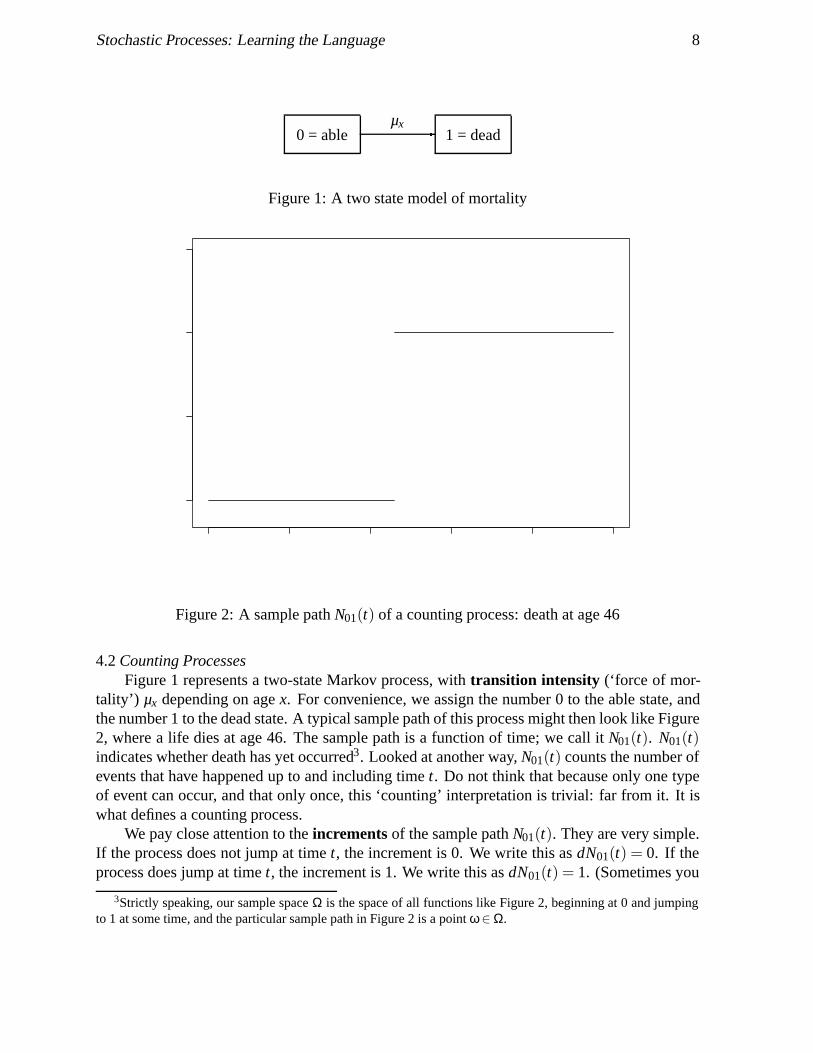
To keep matters clear, we will develop the simplest possible example, represented in anintuitive way by the two-state (or single decrement) model in Figure 1. Of course, this process— death as a single decrement — is very familiar, so at first it seems that all we do is expressfamiliar results in not-so-familiar language. Of itself this offers nothing new, but, we emphasise,the payoff comes when we must model more complicated life histories.(a) All the tools developed in the case of this simple process carry over to more complicated

processes, such as are often needed to model illness or long term care.(b) The useful tools turn out to be exactly those that are also needed in modern financial math-

ematics. In particular, stochastic integrals and conditional expectation are key ideas. So,instead of acquiring two different toolkits, one will do for both.

The main difference between financial mathematics and life insurance mathematics is thatthe former is based on processes with continuous paths, while the latter is based on processeswith jumps2. The fundamental objects in life insurance mathematics are stochastic processescalled ‘counting processes’.

As will be obvious from the references, this section is based on the work of ProfessorRagnar Norberg.

2It might be more accurate to say that, in financial mathematics, the easy examples are provided by continuous-path processes, and discontinuities make the mathematics much harder, while in life insurance mathematics it isthe other way round. However, Norberg (1995b) suggests an interesting alternative point of view.


0 = able 1 = deadµx

Figure 1: A two state model of mortality

Figure 2: A sample path N01(t) of a counting process: death at age 46

4.2 Counting ProcessesFigure 1 represents a two-state Markov process, with transition intensity (‘force of mor-

tality’) µx depending on age x. For convenience, we assign the number 0 to the able state, andthe number 1 to the dead state. A typical sample path of this process might then look like Figure2, where a life dies at age 46. The sample path is a function of time; we call it N01(t). N01(t)indicates whether death has yet occurred3. Looked at another way, N01(t) counts the number ofevents that have happened up to and including time t. Do not think that because only one typeof event can occur, and that only once, this ‘counting’ interpretation is trivial: far from it. It iswhat defines a counting process.

We pay close attention to the increments of the sample path N01(t). They are very simple.If the process does not jump at time t, the increment is 0. We write this as dN01(t) = 0. If theprocess does jump at time t, the increment is 1. We write this as dN01(t) = 1. (Sometimes you

3Strictly speaking, our sample space Ω is the space of all functions like Figure 2, beginning at 0 and jumpingto 1 at some time, and the particular sample path in Figure 2 is a point ω∈ Ω.


will see ∆N01(t) instead of dN01(t); here it does not matter.)Discrete increments like dN01(t) are, for counting processes, what the first derivative d/dx

is for processes with differentiable sample paths. Just as a differentiable sample path can bereconstructed from its derivative (by integration) so can a counting process be reconstructedfrom its increments (also by integration). That leads us to the stochastic integral.

4.3 The Stochastic IntegralBegin with a discrete-time counting process, say one which can jump only at integer times.

Then by definition, dN01(t) = 0 at all non-integer times, and dN01(t) = 1 at no more than oneinteger time. Can we reconstruct N01(t) from its increments dN01(t)? To be specific, can wefind N01(T )? (T need not be an integer). Let J(T ) be the set of all possible jump times up toand including T (that is, all integers ≤ T ). Then:

N01(T ) = ∑t∈J(T )

dN01(t). (1)

Suppose N01(t) is still discrete-time, but can jump at more points: for example at the end ofeach month. Again, define J(T ) as the set of all possible jump times up to and including T , andequation (1) remains valid. This works for any discrete set of possible jump times, no matterhow refined it is (years, months, days, minutes, nanoseconds . . .). What happens in the limit?(a) the counting process becomes the continuous-time version with which we started;(b) the set of possible jump times J(T ) becomes the interval (0,T ]; and(c) the sum for N01(T ) becomes an integral:

N01(T ) =Z

t∈J(T )

dN01(t) =TZ

0

dN01(t). (2)

The integral in equation (2) is a stochastic integral. Regarded as a function of T , it is astochastic process4. This idea is very useful; it lets us write down values of assurances andannuities.

4.4 Assurances and AnnuitiesConsider a whole life assurance paying £1 at the moment of death. What is its present

value at age x (call it X )? In Subjects A2 and 104, one way of writing this down is introduced:define Tx as the time until death of a life aged x (a random variable) and then the present valueof the assurance is X = vTx = e−δTx (in the usual notation).

We can also write this as a stochastic integral. The present value of £1 paid at time t is vt .If the life does not die at time t, the increment of the counting process N is dN01(t) = 0, and thepresent value of the payment is vtdN01(t) = 0. If the life does die at time t, the increment of Nis dN01(t) = 1, and the present value of the payment is vtdN01(t) = vt . Adding up (integrating)we get:

4The stochastic integrals in this section are stochastic just because sample paths of the stochastic process N01(t)are involved in their definitions. Given the sample path of N01(t), these integrals are constructed in the same wayas their deterministic counterparts. The stochastic integrals needed in financial mathematics, called Ito integrals,are a bit different.


X =∞Z

0

vtdN01(t). (3)

Annuities can also be written down as stochastic integrals, with a little more notation.Consider a life annuity of 1 per annum payable continuously, and let Y be its present value.Define a stochastic process I0(t) as follows: I0(t) = 1 if the life is alive at time t, and I0(t) = 0otherwise. This is an indicator process; it takes the value 1 or 0 depending on whether or nota given status is fulfilled. Then:

Y =∞Z

0

vtI0(t)dt. (4)

Given the sample path, this is a perfectly ordinary integral, but since the sample path israndom, so is Y . Defining X(T ) and Y (T ) as the present value of payments up to time T , wecan write down the stochastic processes:

X(T ) =TZ

0

vtdN01(t) and Y (T ) =TZ

0

vtI0(t)dt. (5)

4.5 The Elements of Life Insurance MathematicsGuided by these examples, we can now write down the elements of life insurance math-

ematics in terms of counting processes. This was first done surprisingly recently (Hoem &Aalen, 1978; Ramlau-Hansen 1988; Norberg 1990, 1991). We start with payment functions:(a) if N = 0 at time t (the life is alive), an annuity is payable continuously at rate a0(t) per

annum; and(b) if N jumps from 0 to 1 at time t (the life dies), a sum assured of A01(t) is paid.

Noting the obvious, premiums can be treated as a negative annuity, and these definitions can beextended to any multiple state model. Also without difficulty, discrete annuity or pure endow-ment payments can also be accommodated, but we leave them out for simplicity.

The quantities a0(t) and A01(t) are functions of time, but need not be stochastic processes.They define payments that will be made, depending on events, but they do not represent theevents themselves. In the case of a non-profit assurance, for example, they will be deterministicfunctions of age. The payments actually made can be expressed as a rate, dL(t):

dL(t) = A01(t)dN01(t)+a0(t)I0(t)dt. (6)

This gives the net rate of payment, ‘during’ the time interval t to t + dt, depending on events.We suppose that no payments are made after time T (T could be ∞). The cumulative paymentis then:

L =TZ

0

dL(t) =TZ

0

A01(t)dN01(t)+TZ

0

a0(t)I0(t)dt (7)


and the value of the cumulative payment at time 0, denoted V (0), is:

V (0) =TZ

0

vtdL(t) =TZ

0

vtA01(t)dN01(t)+TZ

0

vta0(t)I0(t)dt (8)

This quantity is the main target of study. Compare it with equation (5); it simply allows formore general payments. It is a stochastic process, as a function of T , since it now represents thepayments made depending on the particular life history (that is, the sample path of N01(t)).

We also make use of the accumulated/discounted value of the payments at any time s,denoted V (s):

V (s) =1vs

TZ

0

vtdL(t) =1vs

TZ

0

vtA01(t)dN01(t)+1vs

TZ

0

vta0(t)I0(t)dt. (9)

4.6 Stochastic Interest RatesAlthough we have written the discount function as vt , implicitly assuming a constant, de-

terministic interest rate, this is not necessary at this stage. We could just as well assume that thediscount function was a function of time, or even a stochastic process. For simplicity, we willnot pursue this, but see Norberg (1991) and Møller (1998).

4.7 Bases and Expected Present ValuesIn terms of probability models, all we have defined so far are the elements of the sample

space Ω (the sample paths N01(t)) and some related functions such as L and V (s). We havenot introduced any σ-algebras, filtrations or probability measures, nor have we carried out anyprobabilistic calculation, such as taking expectations. We now consider these:(a) Our filtration is the ‘natural’ filtration generated by the process N01(t), which is easily

described. At time t, the past values N01(s) (s ≤ t) are all known, and the future valuesN01(s) (s > t) are unknown (unless N01(t) = 1, in which case nothing more can happen).This information is summed up by the σ-algebra Ft .To picture this filtration, cover Figure 2 with your hand, and then slowly reveal the lifehistory. Before age 46, all possible future life histories are hidden by your hand; the infor-mation Ft is the combination of the revealed life history and all these hidden possibilities.

(b) Our ‘overall’ σ-algebra F is the union of all the Ft .(c) The probability measure corresponds to the mortality basis. As is well known, the ac-

tuary will choose a different mortality basis for different purposes, and we suppose thatnature chooses the ‘real’ mortality basis. In other words, the sample space and the filtra-tion do not determine the choice of probability measure; nor is the choice of probabilitymeasure always an attempt to find nature’s ‘real’ probabilities (that is the estimation prob-lem). This point is of even greater importance in financial mathematics, where it is oftenmisunderstood.

All concrete calculations depend on the choice of probability measure (mortality basis). Wewill illustrate this using expected present values. Suppose the actuary has chosen a probabilitymeasure P (equivalent to life table probabilities t px). Taking as an example the whole lifeassurance benefit, for a life aged x, say, EP[X ] is:


SSSSSSw

0 = able 1 = ill

2 = dead

µ01x

µ10x

µ02x µ12

x

Figure 3: An illness-death model

EP

∞Z

0

vtdN01(t)

=

∞Z

0

vtEP[dN01(t)] =∞Z

0

vtP[dN01(t) = 1] =∞Z

0

vtt pxµx+tdt (10)

which should be familiar5. If the actuary chooses a different measure P∗, say (equivalent todifferent life table probabilities t p∗x), we get a different expected value:

EP∗[X ] =∞Z

0

vtt p∗xµ∗x+tdt. (11)

Expected values of annuities are also easily written:

EP[Y ] =∞Z

0

vtt pxdt. (12)

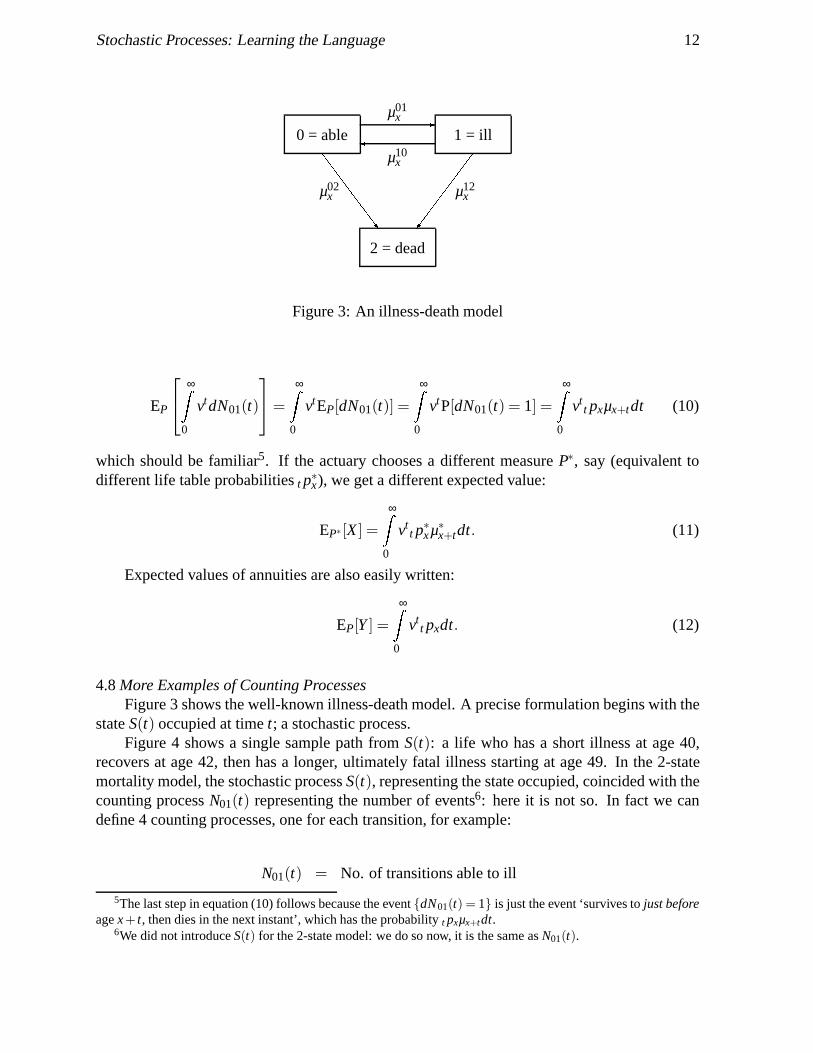
4.8 More Examples of Counting ProcessesFigure 3 shows the well-known illness-death model. A precise formulation begins with the

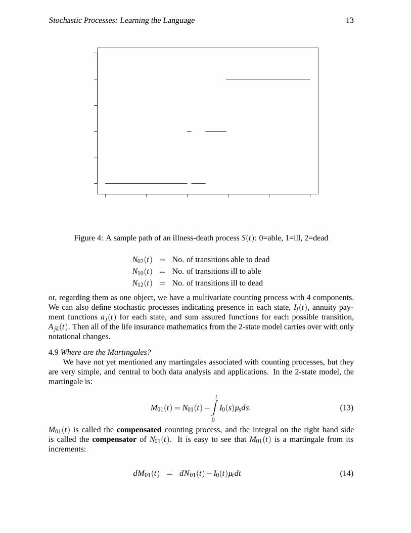
state S(t) occupied at time t; a stochastic process.Figure 4 shows a single sample path from S(t): a life who has a short illness at age 40,

recovers at age 42, then has a longer, ultimately fatal illness starting at age 49. In the 2-statemortality model, the stochastic process S(t), representing the state occupied, coincided with thecounting process N01(t) representing the number of events6: here it is not so. In fact we candefine 4 counting processes, one for each transition, for example:

N01(t) = No. of transitions able to ill

5The last step in equation (10) follows because the event dN01(t) = 1 is just the event ‘survives to just beforeage x+ t, then dies in the next instant’, which has the probability t pxµx+tdt.

6We did not introduce S(t) for the 2-state model: we do so now, it is the same as N01(t).


Figure 4: A sample path of an illness-death process S(t): 0=able, 1=ill, 2=dead

N02(t) = No. of transitions able to dead

N10(t) = No. of transitions ill to able

N12(t) = No. of transitions ill to dead

or, regarding them as one object, we have a multivariate counting process with 4 components.We can also define stochastic processes indicating presence in each state, Ij(t), annuity pay-ment functions a j(t) for each state, and sum assured functions for each possible transition,Ajk(t). Then all of the life insurance mathematics from the 2-state model carries over with onlynotational changes.

4.9 Where are the Martingales?We have not yet mentioned any martingales associated with counting processes, but they

are very simple, and central to both data analysis and applications. In the 2-state model, themartingale is:

M01(t) = N01(t)−tZ

0

I0(s)µsds. (13)

M01(t) is called the compensated counting process, and the integral on the right hand sideis called the compensator of N01(t). It is easy to see that M01(t) is a martingale from itsincrements:

dM01(t) = dN01(t)− I0(t)µtdt (14)


EP[dM01(t)] = EP[dN01(t)]−EP[I0(t)µtdt] = 0 (15)

We have been careful to specify the probability measure P in the expectation. If we changethe measure, for example to P∗, corresponding to probabilities t p∗x , we get a different martingale:

M∗01(t) = N01(t)−

tZ

0

I0(s)µ∗sds (16)

and EP∗[dM∗01(t)] = 0. Alternatively, given a force of mortality µ∗t , we can find a probability

measure P∗ such that M∗01(t) is a P∗-martingale; P∗ is simply given by the probabilities t p∗x =

exp(−R t

0 µ∗s ds). This is true of any (well-behaved) force of mortality, not just nature’s chosen‘true’ force of mortality7.

An idea of the usefulness of M01(t) can be gained from equation (13). If we consider anage interval short enough that a constant transition intensity µ is a reasonable approximation,this becomes:

M01(t) = N01(t)−µ

tZ

0

I0(s)ds. (17)

But the two random quantities on the right are just the number of deaths N01(t), and the totaltime spent at risk

R t0 I0(s)ds, better known as the central exposed to risk. All the properties

of the maximum likelihood estimate of µ, based on these two statistics (summed over manyindependent lives) are consequences of the fact that M01(t) is a martingale (see Macdonald(1996a, 1996b)).

For more complicated models, we get a set of martingales, one for each possible transition(from state j to state k) of the form:

Mjk(t) = Njk(t)−tZ

0

I j(s)µ jks ds (18)

which have all the same properties.

4.10 Prospective and Retrospective ReservesWe now return to equation (9): V (s) = v−s R T

0 vtdL(t). Recall that the premium is partof the payment function a0(t); setting the premium according to the equivalence principlesimply means setting EP[V (0)] = 0 and solving for a0(t), where P is the probability measurecorresponding to the premium basis.

For convenience, we will use the same basis (measure) for premiums and reserves, as iscommon in other European countries.

Reserves follow when we consider the evolution of the value function V over time, asinformation emerges. We start from the conditional expectation; for s < T :

7This is exactly analogous to the ‘equivalent martingale measure’ of financial mathematics, in which we aregiven the drift of a geometric Brownian motion (coincidentally, also often denoted µt ) and then find a probabilitymeasure under which the discounted process is a martingale.


EP[V (s)|Fs] = EP

1

vs

TZ

0

vtdL(t)∣∣∣∣ Fs

(19)

= EP

1

vs

sZ

0


+EP

1

vs

TZ

s


(20)

The second term on the right is the prospective reserve at time s. If the information Fs isthe complete life history up to time s, it is the same as the usual prospective reserve. However,this definition is more general; for example, under a joint-life second-death assurance, the firstdeath might not be reported, so that Fs represents incomplete information. Also, it does notdepend on the probabilistic nature of the process generating the life history; it is not necessaryto suppose that the process is Markov, for example. If the process is Markov (as we oftensuppose) then conditioning on Fs simply means conditioning on the state occupied at time s,which is very convenient in practice.

The first term on the right is minus the retrospective reserve. This definition of the retro-spective reserve is new (Norberg, 1991) and is not equivalent to ‘classical’ definitions. This isa striking achievement of the stochastic process approach: for convenience we also list some ofthe notions of retrospective reserve that have preceded it:(a) The ‘classical’ retrospective reserve (for example, Neill (1977)) depends on a deterministic

cohort of lives, who share out a fund among survivors at the end of the term. However,this just exposes the weaknesses of the deterministic model: given a whole number of livesat outset, lx say, the number of survivors some time later, lxt px is usually not an integer.Viewed prospectively this can be excused as being a convenient way of thinking aboutexpected values, but viewed retrospectively there is no such excuse.

(b) Hoem (1969) allowed both the number of survivors, and the fund shared among survivors,to be random, and showed that the classical retrospective reserve was obtained in the limit,as the number of lives increased to infinity.

(c) Perhaps surprisingly, the ‘classical’ notion of retrospective reserve does not lead to a uniquespecification of what the reserve should be in each state of a general Markov model, leadingto several alternative definitions (Hoem, 1988; Wolthius & Hoem, 1990; Wolthius, 1992)in which the retrospective and prospective reserves in the initial state were equated bydefinition.

(d) Finally, Norberg (1991) pointed out that the ‘classical’ retrospective reserve is “. . . rather aretrospective formula for the prospective reserve . . .”, and introduced the definition in equa-tion (20). This is properly defined for individual lives, and depends on known informationFs. If Fs is the complete life history, the conditional expectation disappears and:

Retrospective reserve =−1vs

sZ

0

vtdL(t) (21)

which is more akin to an asset share on an individual policy basis. If Fs represents coarserinformation, for example aggregate data in respect of a cohort of policies, the retrospectivereserve is akin to an asset share with pooling of mortality costs.


We have spent some time on retrospective reserves, because it is an example of the greaterclarity obtained from a careful mathematical formulation of the process being modelled, in thiscase the life history.

4.11 Differential EquationsThe chief computational tools associated with multiple-state models are ordinary differ-

ential equations (ODEs). We mention three useful systems of ODEs:(a) The Kolmogorov forward equations can be found in any textbook on Markov processes

(for example, Kulkarni (1995)) and have been in the actuarial syllabus for some time. Theyallow us to calculate transition probabilities in a Markov process, given the transition in-tensities, which is exactly what we need since transition intensities are the quantities mosteasily estimated from data. We give just one example, the simplest of all from the 2-statemodel:

∂∂t t px = −t pxµx+t . (22)

(b) Theile’s equation governs the development of the prospective reserve. For example, if tV xis the reserve under a whole life assurance for £1, Theile’s equation is:

ddt tV x = δtV x +Px − (1− tV x)µx+t (23)

which has a very intuitive interpretation. In fact, it is the continuous-time equivalent ofthe recursive formula for reserves well-known to British actuaries. It was extended to anyMarkov model by Hoem (1969).

(c) Norberg (1995b) extended Theile’s equations for prospective policy values (that is, firstmoments of present values) to second and higher moments. We do not show these equa-tions, as that would need too much new notation, but we note that they were obtained fromthe properties of counting process martingales.

Most systems of ODEs do not admit closed-form solutions, and have to be solved nu-merically, but many methods of solution are quite simple8, and well within the capability of amodern PC. So, while closed-form solutions are nice, they are not too important, and it is betterto seek ODEs that are relevant to the problem, rather than explicitly soluble. We would remindactuaries of a venerable example of a numerical solution to an intractable ODE, namely the lifetable.

4.12 Advantages of the Counting Process Approach(a) First and foremost, counting processes represent complete life histories. In practice, not

all this information might be available or useable, but it is best to start with a model thatrepresents the underlying process, and then to make whatever approximations might beneeded to meet the circumstances (for example, data grouped into years).

(b) The mathematics of counting processes and multiple-state models is easily introduced interms of the 2-state mortality model, but carries over to any more complicated model, thussolving problems that defeat life-table methods. This is increasingly important in practice,as new insurances are introduced.

8Numerical solution of ODEs is one of the most basic tasks in numerical analysis.


(c) Completely new results have been obtained, such as an operational definition of retrospec-tive reserves, and Norberg’s differential equations.

(d) The tools we use are exactly those that are essential in modern financial mathematics, inparticular stochastic integrals and conditional expectations. For a remarkable synthesis ofthese two fields, see Møller (1998). An alternative approach, in which rates of return aswell as lifetimes are modelled by Markov processes, has been developed (Norberg, 1995b)extending greatly the scope of the material discussed here.

(e) We have not discussed data analysis, but mortality studies are increasingly turning towardscounting process tools, for exactly the same reason as in (a). It will often be helpful foractuaries at least to understand the language.

5. FINANCE

5.1 IntroductionIn this section we are going to illustrate how stochastic processes can be used to price

financial derivatives.A financial derivative is a contract which derives its value from some underlying security.

For example, a European call option on a share gives the holder the right, but not the obligation,to buy the share at the exercise date T at the strike price of K. If the share price at time T , ST ,is less than K then the option will not be exercised and it will expire without any value. If ST isgreater than K then the holder will exercise the option and a profit of ST −K will be made. Theprofit at T is, therefore, maxST −K,0.

5.2 Models of Asset PricesMuch of financial mathematics must be based on explicit models of asset prices, and the

results we get depend on the models we decide to use. In this section we will look at two modelsfor share prices: a simple binomial model which will bring out the main points; and geometricBrownian motion. Throughout we make the following general assumptions9.(a) We will use St to represent the price of a non-dividend-paying stock at time t (t = 0,1,2, . . .).

For t > 0, St is random.(b) Besides the stock we can also invest in a bond or a cash account which has value Bt at time

t per unit invested at time 0. This account is assumed to be risk free and we will assume thatit earns interest at the constant risk-free continuously compounding rate of r per annum.Thus Bt = exp(rt). (In discrete time, risk free means that we know at time t −1 what thevalue of the risk-free investment will be at time t. In this more simple case, the value of therisk-free investment at any time t is known at time 0.)

(c) At any point in time we can hold arbitrarily large amounts (positive or negative) of stock orcash.

5.3 The No-Arbitrage PrincipleBefore we progress it is necessary to discuss arbitrage.

9These assumptions can be relaxed considerably with more work.


Suppose that we have a set of assets in which we can invest (with holdings which can bepositive or negative). Consider a particular portfolio which starts off with value zero at time 0(so we have some positive holdings and some negative). With this portfolio, it is known thatthere is some time T in the future when its value will be non-negative with certainty and strictlypositive with probability greater than zero. This is called an arbitrage opportunity. To exploit itwe could multiply up all amounts by one thousand or one million and make huge profits withoutany cost or risk.

In financial mathematics and derivative pricing we make the fundamental assumption thatarbitrage opportunities like this do not exist (or at least that if they do exist, they disappear tooquickly to be exploited).

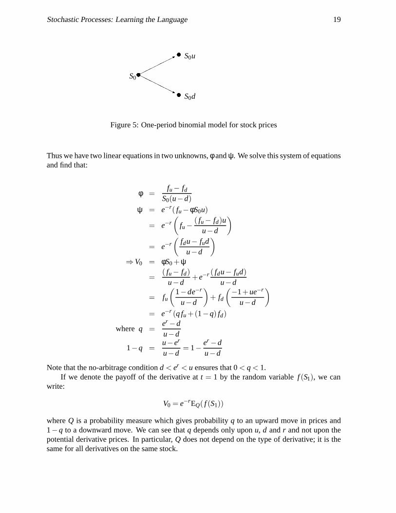
5.4 A One-Period Binomial ModelFirst we consider a model for stock prices over one discrete time period. We have two

possibilities for the price at time 1 (see Figure 5):

S1 =

S0u if the price goes upS0d if the price goes down

with d < u (strictly, it is not necessary that d < 1).In order to avoid arbitrage we must have d < er < u. Suppose this is not the case: for

example, if er < d. Then we could borrow £1 of cash and buy £1 of stock. At time 0 this wouldhave a net cost of £0. At time 1 our portfolio would be worth d −er or u−er both of which aregreater than 0: an example of arbitrage.

Suppose that we have a derivative which pays fu if the price of the underlying stock goesup and fd if the price of the underlying stock goes down. At what price should this derivativetrade at time 0?

In this model (and also in the multi-period model that we consider later) we will assume:(a) there are no trading costs;(b) there are no minimum or maximum units of trading;(c) stock and bonds can only be bought and sold at discrete times 1, 2, ...

As such the model appears to be quite unrealistic. However, it does provide us with good insightinto the theory behind more realistic models. Furthermore it provides us with an effectivecomputational tool for derivatives pricing.

At time 0 suppose we hold φunits of stock and ψ units of cash. The value of this portfolioat time 0 is V0. At time 1 the same portfolio has the value:

V1 =

φS0u+ψer if the stock price goes upφS0d +ψer if the stock price goes down

Let us choose φ and ψ so that V1 = fu if the stock price goes up and V1 = fd if the stockprice goes down. Then:

φS0u+ψer = fu

and φS0d +ψer = fd


HHHHHHj

u

u

u

S0

S0u

S0d

Figure 5: One-period binomial model for stock prices

Thus we have two linear equations in two unknowns, φand ψ. We solve this system of equationsand find that:

φ =fu − fd

S0(u−d)ψ = e−r( fu −φS0u)

= e−r(

fu −( fu − fd)u

u−d

)

= e−r(

fdu− fudu−d

)

⇒V0 = φS0 +ψ

=( fu − fd)

u−d+e−r ( fdu− fud)

u−d

= fu

(1−de−r

u−d

)+ fd

(−1+ue−r

u−d

)

= e−r (q fu +(1−q) fd)

where q =er −du−d

1−q =u−er

u−d= 1− er −d

u−d

Note that the no-arbitrage condition d < er < u ensures that 0 < q < 1.If we denote the payoff of the derivative at t = 1 by the random variable f (S1), we can

write:

V0 = e−rEQ( f (S1))

where Q is a probability measure which gives probability q to an upward move in prices and1−q to a downward move. We can see that q depends only upon u, d and r and not upon thepotential derivative prices. In particular, Q does not depend on the type of derivative; it is thesame for all derivatives on the same stock.


The portfolio (φ,ψ) is called a replicating portfolio because it replicates, precisely, thepayoff at time 1 on the derivative without any risk. It is also a simple example of a hedgingstrategy: that is, an investment strategy which reduces the amount of risk carried by the issuerof the contract. In this respect not all hedging strategies are replicating strategies.

Up until now we have not mentioned the real-world probabilities of up and down movesin prices. Let these be p and 1− p where 0 < p < 1, defining a probability measure P.

Other than by total coincidence, p will not be equal to q.Let us consider the expected stock price at time 1. Under P this is:

S0(pu+(1− p)d) = EP(S1)

and under Q it is:

EQ(S1) = S0(qu+(1−q)d) = S0

(u(er −d)

u−d+

d(u−er)u−d

)= S0er.

Under Q we see that the expected return on the risky stock is the same as that on a risk-freeinvestment in cash. In other words under the probability measure Q investors are neutral withregard to risk: they require no additional returns for taking on more risk. This is why Q issometimes referred to as a risk-neutral probability measure.

Under the real-world measure P the expected return on the stock will not normally be equalto the return on risk-free cash. Under normal circumstances investors demand higher expectedreturns in return for accepting the risk in the stock price. Thus we would normally find thatp > q. However, this makes no difference to our analysis.

5.5 Comparison of Actuarial and Financial Economic ApproachesThe actuarial approach to the pricing of this contract would give:

V a0 = e−δEP[ f (S1)] = e−δ(p fu +(1− p) fd)

where δ is the actuarial, risk-discount rate. Compare this with the price calculated using theprinciples of financial economics above:

V0 = e−rEQ( f (S1)) = e−r(q fu +(1−q) fd).

If forwards are trading at Va0 , where V a

0 >V0, then we can sell one derivative at the actuarialprice, and use an amount V0 to set up the replicating portfolio (φ,ψ) at time 0. The replicatingportfolio ensures that we have the right amount of money at t = 1 to pay off the holder of thederivative contract. The difference between Va

0 and V0 is then guaranteed profit with no risk.Similarly if V a

0 < V0 we can also make arbitrage profits.(In fact neither of these situations could persist for any length of time because demand for

such contracts trading at Va0 would push the price back towards V0 very quickly. This is a funda-

mental principle of financial economics: that is, prices should not admit arbitrage opportunities.If they did exist then the market would spot any opportunities very quickly and the resultingexcess supply or demand would remove the arbitrage opportunity before any substantial profitscould be made. In other words, arbitrage opportunities might exist for very short periods of time


in practice, while the market is free from arbitrage for the great majority of time and certainly atany points in time where large financial transactions are concerned. Of course, we would haveno problem in buying such a contract if we were to offer a price of Va

0 to the seller if this wasgreater than V0 but we would not be able to sell at that price. Similarly we could easily sell sucha contract if V a

0 <V0 but not buy at that price. In both cases we would be left in a position wherewe would have to maintain a risky portfolio in order to give ourselves a chance of a profit, sincehedging would result in a guaranteed loss.)

For V a0 to make reasonable sense, then, we must set δ in such a way that Va

0 equals V0. Inother words, the subjective choice of δ in actuarial work equates to the objective selection ofthe risk-neutral probability measure Q. Choosing δ to equate Va

0 and V0 is not what happensin practice and, although δ is set with regard to the level of risk under the derivative contract,the subjective element in this choice means that there is no guarantee that Va

0 will equal V0. Ingeneral, therefore, the actuarial approach, on its own, is not appropriate for use in derivativepricing. Where models are generalised and assumptions weakened to such an extent that it isnot possible to construct hedging strategies which replicate derivative payoffs then there is arole for a combination of the financial economic and actuarial approaches. However, this isbeyond the scope of this paper.

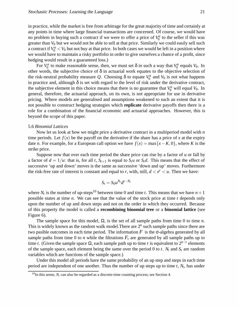
5.6 Binomial LatticesNow let us look at how we might price a derivative contract in a multiperiod model with n

time periods. Let f (x) be the payoff on the derivative if the share has a price of x at the expirydate n. For example, for a European call option we have f (x) = maxx−K,0, where K is thestrike price.

Suppose now that over each time period the share price can rise by a factor of u or fall bya factor of d = 1/u: that is, for all t, St+1 is equal to Stu or Std. This means that the effect ofsuccessive ‘up and down’ moves is the same as successive ‘down and up’ moves. Furthermorethe risk-free rate of interest is constant and equal to r, with, still, d < er < u. Then we have:

St = S0uNt dt−Nt

where Nt is the number of up-steps10 between time 0 and time t. This means that we have n+1possible states at time n. We can see that the value of the stock price at time t depends onlyupon the number of up and down steps and not on the order in which they occurred. Becauseof this property the model is called a recombining binomial tree or a binomial lattice (seeFigure 6).

The sample space for this model, Ω, is the set of all sample paths from time 0 to time n.This is widely known as the random walk model.There are 2n such sample paths since there aretwo pssible outcomes in each time period. The information F is the σ-algebra generated by allsample paths from time 0 to n while the filtrations Ft are generated by all sample paths up totime t. (Given the sample space Ω, each sample path up to time t is equivalent to 2n−t elementsof the sample space, each element being the same over the period 0 to t. Nt and St are randomvariables which are functions of the sample space.)

Under this model all periods have the same probability of an up step and steps in each timeperiod are independent of one another. Thus the number of up steps up to time t, Nt , has under

10In this sense, Nt can also be regarded as a discrete-time counting process; see Section 4.


uS0

HHHHHHj

u S0u

HHHHHHj

u S0d

HHHHHHj

u S0u2

HHHHHHj

u S0ud

HHHHHHj

u S0d2

HHHHHHj

u S0u3

HHHHHHj

u S0u2d

HHHHHHj

u S0ud2

HHHHHHj

u S0d3

HHHHHHj

u S0u4

u S0u3d

u S0u2d2

u S0ud3

u S0d4

Figure 6: Recombining binomial tree or binomial lattice

Q a binomial distribution with parameters t and q. Furthermore, for 0 < t < n, Nt is independentof Nn −Nt and Nn −Nt has a binomial distribution with parameters n− t and q.

Let us extend our notation a little bit. Let Vt( j) be the fair value of the derivative at time tgiven Nt = j for j = 0, . . . , t. Also let Vn( j) = f

(S0u jdn− j

). Finally we write Vt = Vt(Nt) to be

the random value at some future time t.In order for us to calculate the value at time 0, V0(0), we must work backwards one period

at a time from time n making use of the one-period binomial model as we go.First let us consider the time period n−1 to n. Suppose that Nn−1 = j. Then, by analogy

with the one-period model we have:

Vn−1( j) = e−r [qVn( j +1)+(1−q)Vn( j)]= e−rEQ [Vn | Fn−1]= e−rEQ [ f (Sn) | Nn−1 = j]= e−rEQ [ f (Sn) | Fn−1]

where q =er −du−d

.


Equivalently we can write this as Vn−1 = e−rEQ[ f (Sn) | Fn−1].As we work backwards we have:

Vt−1 = e−rEQ[Vt | Ft−1]= e−rEQ

[e−rEQ (Vt+1 | Ft) | Ft−1

]= e−2rEQ [Vt+1 | Ft−1] (using the Tower Law)...

......

= e−(n−t+1)rEQ [Vn | Ft−1]

= e−(n−t+1)rEQ [ f (Sn) | Ft−1] .

Finally we get to:

V0 = e−nrEQ [ f (Sn) | F0] = e−nrEQ [ f (Sn) | S0] .

The price at time t of the path-dependent derivative is thus:

Vt = e−r(n−t)EQ

[f(

StuNn−Nt d(n−t)−(Nn−Nt)

)| Nt

]

= e−r(n−t)n−t

∑k=0

f(

Stukdn−t−k

) (n− t)!k!(n− t −k)!

qk(1−q)n−t−k.

We have noted before that EQ(S1) = S0er giving rise to the use of the name risk-neutralmeasure for Q. Similarly in the n-period model we have (putting f (s) = s):

EQ[St |F0] = S0ert .

So the use of the expression risk-neutral measure for Q is still valid. Alternatively we canwrite:

EQ[e−rT ST | Ft

]= e−rtSt .

In other words, the discounted asset value process Dt = e−rtSt is a martingale under Q. Thisgives rise to another name for Q: equivalent martingale measure.

In fact we normally use this result the other way round, as we will see in the next section.That is, the first thing we do is to find the equivalent martingale measure Q, and then use itimmediately to price derivatives.

5.7 A Continuous-Time ModelLet us now work in continuous time. Let St be the price of the non-dividend-paying share

for 0 ≤ t ≤ T . Suppose that a derivative pays f (s) at time T if the share price at time T is equalto s.


The particular model we are going to look at for St is called geometric Brownian motion:that is, St = S0 exp[(µ− 1

2σ2)t +σZt ] where Zt is a standard Brownian motion under the real-world measure P. (For the properties of Brownian motion see Appendix A.) This means thatSt has a log-normal distribution with mean S0 exp(µt) and variance exp(2µt).

[exp(σ2t)−1

].

By application of Ito’s lemma (see Appendix B) we can write down the stochastic differentialequation (SDE) for St as follows:

dSt = µStdt +σStdZt .

By analogy with the binomial model there is another probability measure Q (the risk-neutralmeasure or equivalent martingale measure) under which:(a) e−rtSt is a martingale(b) St can be written as the geometric Brownian motion S0 exp

[(r− 1

2σ2)

t +σZt]

where Z(t)is a standard Brownian motion under Q

By continuing the analogy with the binomial model (for example, see Baxter & Rennie(1996)) we can also say that the value at time t of the derivative is:

Vt = e−r(T−t)EQ [ f (ST ) | Ft ] = e−r(T−t)EQ [ f (ST ) | St ] .

With a bit more work we can also see that, under this model, if we invest Vt in the rightway (that is, with a suitable hedging strategy), then we can replicate the payoff at T without theneed for extra cash.

Suppose that we consider a European call option, so that f (s) = maxs−K,0. Then wecan exploit a well known property of the log-normal distribution to get the celebrated Black-Scholes formula:

Vt = StΦ(d1)−Ke−r(T−t)Φ(d2)

where d1 =log St

K +(r + 1

2σ2)(T − t)

σ√

T − t

and d2 = d1 −σ√

T − t.

A more detailed development of pricing and hedging of derivatives in continuous time canbe found in Baxter & Rennie (1996).

6. APPLICATIONS IN RISK THEORY

6.1 IntroductionIn this section we show how stochastic processes can be used to gain insight into the pricing

of general insurance policies. In particular, we will make use of the notion of a martingale,Brownian motion and also the optional stopping theorem.

Suppose we have a general insurance risk, for example comprehensive insurance for afleet of cars or professional indemnity insurance for a software supplier, for which cover isrequired on an annual basis. We want to answer the question: “In an ideal world, how should


we calculate the annual premium for this cover?” Let us denote by Pn the premium to becharged for cover in year n, where the coming year is year 1.

The starting point is to consider the claims which will arise each year. Since the aggregateamount of claims is uncertain, we model these amounts as random variables. Let Sn be a randomvariable denoting the aggregate claims arising from the risk in year n. We might also take intoconsideration, particularly for a large risk, the amount of capital with which we are preparedto back this risk. We denote this initial capital, or ‘initial surplus’, U . In practice, we wouldalso take into consideration many other factors, for example, expenses and the premium ratescharged by our competitors. However, to keep things simple, we will ignore these other factors.

Throughout this section we will assume that the random variables Sn∞n=1 are independent

of each other, but we will not assume they are identically distributed. To be able to calculatePn we need to be able to calculate, or at least estimate, the distribution of Sn. If we haveinformation about the distributions of claim numbers and claim amounts in year n, we maybe able to use Panjer’s celebrated recursion formula to calculate the distribution of Sn. See,for example, Klugman et al (1997). In some circumstances, for example, when Sn is the sumof a large number of independent claim amounts, it may be reasonable to assume that Sn has,approximately, a normal distribution. In what follows we will occasionally make the followingassumption:

Sn ∼ N(µn,σ2n) (24)

for some parameters µn and σn.

6.2 The Standard Deviation PrincipleSuppose we decide that each year Pn should be set at a level such that the probability that

aggregate claims exceed the premium in that year should be suitably small, say 1− p. Formally,this criterion can be expressed as follows:

P[Sn < Pn] = p. (25)

Making the additional assumption that Sn is normally distributed, that is, assumption (24),it is easy to see that:

Pn = µn +γpσn (26)

where γp is such that:

Φ(γp) = p

and Φ(z) is the cumulative distribution function of the N(0,1) distribution.Formula (26) says that in year n, Pn should be calculated as the mean of the aggregate claims

for that year plus a loading proportional to the standard deviation of the aggregate claims. Noticethat the proportionality factor, γp, does not depend on n. In the actuarial literature, formula (26)is known as the standard deviation principle for the calculation of premiums, and γp is referredto as the loading factor. See Goovaerts, De Vylder, & Haezendonck (1984).


6.3 Utility Functions and the Variance PrincipleNow suppose that our attitude to money is summarised by a utility function, u(x). Intu-

itively, u(x) is a real-valued function which expresses ‘how much we like an amount of moneyx’. Mathematically, we require the following two conditions to hold:

ddx

u(x) > 0 andd2

dx2 u(x) < 0.

The first of these conditions says that “we always prefer more money”. The second conditionsays that “an extra pound is worth less, the wealthier we are”. See Bowers et al. (1997) formore details.

We can use this utility function to calculate Pn from the following formula:

u(W ) = E[u(W +Pn −Sn)] (27)

where W is our wealth at the start of the n-th year. The rationale behind this formula is asfollows: if we do not insure this risk, the utility of our wealth is u(W ); if we do insure the risk,our expected utility of wealth at the end of the year is E[u(W + Pn − Sn)]. Formula (27) saysthat for a premium of Pn we are indifferent between insuring the risk and not insuring it. In thissense the premium Pn is ‘fair’. See, for example, Bowers et al. (1997) for details.

Now assume that u(x) is an exponential utility function with parameter α > 0, so that:

u(x) = 1−e−αx. (28)

Using (28) in (27) and solving for Pn, we have:

Pn = α−1 log(MSn(α)) (29)

where the notation MZ(.) denotes the moment generating function of a random variable Z, sothat MZ(α) = E[eαZ]. Notice that in this special case Pn does not depend on W , our wealth atthe start of the n-th year.

Finally, let us assume that Sn has a normal distribution, as in (24). Then:

MSn(α) = expµnα +12

α2σ2n

and so (29) becomes:

Pn = µn +12

ασ2n. (30)

Thus, Pn is calculated according to the variance principle.


6.4 Multi-period Analysis — Discrete TimeFormulae (26) and (30) provide two alternative ways of calculating Pn in an ideal world.

They have some features in common:(a) in each case Pn is the sum of the expected value of Sn and a positive loading; and(b) in each case we arrived at a formula for Pn by considering the n-th year in isolation from

any other years.

A major difference in the development so far is that for (26) the loading factor γp has an intuitivemeaning, whereas in (30), or (29), the parameter α is not so easily understood or quantified. Tofill in this gap, we need to consider our surplus at the end of each year in the future.

Let Un denote the surplus at the end of the n-th year, so that:

Un = U +n

∑k=1

(Pk −Sk)

for n = 1,2,3, . . ., with U0 defined to be U . Now define:

ψ(U) = P[Un ≤ 0 for some n, n = 1,2,3, . . .]

to be the probability that at some time in the future we will need more capital to back this risk,that is, in more emotive language, the probability of ultimate ruin in discrete time for our surplusprocess. Let us assume that Pn is calculated using (29).

Consider the process Yn∞n=0, where Yn = exp−αUn for n = 0,1,2, ... . Then Yn∞

n=0 isa martingale with respect to Sn∞

n=1. To prove this, note that:

Un+1 = Un +Pn+1 −Sn+1

implies that:

E [Yn+1|S1, . . . ,Sn]= E [exp−α (Un +Pn+1 −Sn+1) |S1, . . . ,Sn]= E [exp−α(Pn+1−Sn+1)|S1, . . . ,Sn]exp−αUn.

Since Sn∞n=1 is a sequence of independent random variables it follows that:

E [exp−α(Pn+1−Sn+1)|S1, . . . ,Sn]= E[exp−α(Pn+1 −Sn+1)]= exp−αPn+1E [expαSn+1]= 1

where the final step follows from (29). Hence:

E [Yn+1|S1, ...,Sn] = exp−αUn = Yn,


and so the proof is complete.We can now use this fact to find a bound for ψ(U). To do so, let us introduce the positive

constant b > U , and define the stopping time T by:

T = min(n: Un ≤ 0 or Un ≥ b) :

Thus, the process stops when the first of two events occurs: (i) ruin; or, (ii) the surplus reachesat least level b. The optional stopping theorem tells us that:

E [exp−αUT] = exp−αU.

Let pb denote the probability that ruin occurs without the surplus ever having been at levelb or above. Then, conditioning on the two events described above:

E [exp−αUT] = E [exp−αUT|UT ≤ 0] pb

+E [exp−αUT|UT ≥ b] (1− pb) (31)

= exp−αU.

Now let b → ∞. Then pb → ψ(u), the first expectation on the right hand side of (31) is atleast 1 since it is the moment generating function of the deficit at ruin, evaluated at α, and thesecond expectation goes to 0 since it is bounded above by exp−αb. Thus:

exp−αU = ψ(U)E [exp−αUT|UT ≤ 0]

giving:

ψ(U) =exp−αU

E [exp−αUT|UT ≤ 0]≤ exp−αU. (32)

This gives us a simple bound on the probability of ultimate ruin. It also suggests an appro-priate value for the parameter α in formula (29). For example, if the initial surplus is 10, and werequire that the probability of ultimate ruin is to be no more than 1%, then we require α suchthat exp−10α = 0.01, giving α = 0.461.

Let us consider the special case when Sn∞n=1 is a sequence of independent and identically

distributed random variables, each distributed as compound Poisson with Poisson parameter λ.Then Pn is independent of n, say Pn = P, and:

P = α−1 logE [expαSn]= α−1 log [expλ (MX(α)−1)]

where MX(.) is the moment generating function of the distribution of a single claim amount,giving:

λ +Pα = λMX(α). (33)


This is the equation for the adjustment coefficient for this model (see, for example, Gerber(1979)). Thus, in this particular case, the parameter α is the adjustment coefficient, and equation(32) is simply Lundberg’s inequality.

6.5 Multi-period Analysis — Continuous TimeFormula (32) shows that when the annual premium is calculated according to formula (29),

the probability of ultimate ruin in discrete time for our surplus process is bounded above byexp−αU. If, in addition, the distribution of aggregate claims each year is normal (assumption(24)) then formula (29) implies that the premium loading is proportional to the variance of theaggregate claims.

We can gain a little more insight, particularly into formula (32), by moving from a discretetime model to a continuous time model. In this section we assume that the aggregate claims inthe time interval [0, t] are a random variable µt +σB(t), where the stochastic process B(t)t≥0

is standard Brownian motion (see Appendix A). This means that in any year, the aggregateclaims are distributed as N(µ,σ2), and are independent of the claims in any other year. Thisis the continuous time version of assumption (24), but note that we are now assuming that themean and variance of the annual aggregate claims do not change over time. Brownian motionhas stationary and independent increments so for any 0 ≤ s < t:

B(t)−B(s)∼ N((t − s)µ,(t− s)σ2) . (34)

We assume that premiums are received continuously at constant rate P per annum, where:

P = µ+12

ασ2 (35)

which is equivalent to formula (30). The surplus at time t is denoted U(t), where:

U(t) = U +Pt − (µt +σB(t)). (36)

Now let:

ψc(U) = P[U(t)≤ 0 for some t, t > 0]

so that ψc(U) is the probability of ultimate ruin in continuous time for our surplus process. Wewill apply the martingale argument of the previous subsection to find ψc(U). First note that:

E[exp−α((P−µ)t −σB(t))] = 1. (37)

This follows from formulae (34) and (35) and the formula for the moment generating functionof the normal distribution.

Next, let Y (t) = E[exp−αU(t)]. Then the process Y (t)t≥0 is a martingale with re-spect to11 B(t)t≥0. (Since U(t)t≥0 is a continuous time stochastic process, Y (t)t≥0 is amartingale in continuous time.) This follows since for t > s:

11Recall that a martingale is defined with respect to a filtration: here we mean that the relevant filtration is thatgenerated by the process B(t)t≥0.


E[Y (t)|B(u), 0 ≤ u ≤ s]= E[exp−αU(t)|B(u), 0 ≤ u ≤ s]= E[exp−α(U(t)−U(s))exp−αU(s)|B(u), 0 ≤ u ≤ s].

Hence:

E[Y (t)|B(u), 0 ≤ u ≤ s]= E[exp−α(U(t)−U(s))|B(u), 0 ≤ u ≤ s]E[exp−αU(s)|B(u), 0 ≤ u ≤ s]= E[exp−α(U(t)−U(s))]exp−αU(s).

Now:

U(t)−U(s) = (P−µ)(t − s)−σ(B(t)−B(s)).

We can then use the fact that the process B(t)t≥0 has stationary increments to say that B(t)−B(s) is equivalent in distribution to B(t − s), and hence U(t)−U(s) is equivalent in distributionto U(t − s)−U . (All that stationarity implies is that the distribution of the increment of aprocess over a given time interval depends only on the length of that time interval, and not onits location. In our context, we are simply interested in the increment of the process B(t)t≥0

in a time interval of length t − s.) Hence:

E[exp−α(U(t)−U(s))]= E[exp−α (U(t − s)−U)]= E [exp−α ((P−µ)(t − s)+σB(t − s))]= 1

where the final step follows from (37). Hence:

E[Y (t)|B(u), 0 ≤ u ≤ s] = exp−αU(s) = Y (s)

and so Y (t)t≥0 is a martingale with respect to B(t)t≥0.The optional stopping theorem also applies to martingales in continuous time, so we can

use the same argument as in the previous subsection. We define:

Tc = inft: U(t)≤ 0 or U(t)≥ b)

where b > U . From the optional stopping theorem we have:

E [exp−αU(Tc)] = exp−αU.

Once again defining pb to be the probability that ruin occurs without the surplus process everhaving been at level b or above, we have:


E [exp−αU(Tc)] = E [exp−αU(Tc)|U(Tc) ≤ 0] pb

+E [exp−αU(Tc)|U(Tc) ≥ b] (1− pb)= exp−αU.

If the surplus level attains b without ruin occurring, then U(Tc) = b since the sample paths ofBrownian motion are continuous, i.e. the process cannot jump from below b to above b withoutpassing through b. The situation is the same if ruin occurs. Hence:

E [exp−αU(Tc)|U(Tc) ≥ b] = exp−αb

and:

E [exp−αU(Tc)|U(Tc) ≤ 0] = 1.

Thus:

pb +exp−αb(1− pb) = exp−αU

and if we let b → ∞, then pb → ψc(U), and hence:

ψc(U) = exp−αU. (38)

Formula (38) is Lundberg’s inequality for our continuous time surplus process, but this isnow an equality. Going back to formula (32), this shows that the upper bound for the probabilityof ruin in discrete time, in the special case where the mean and variance of claims do not changeover time, is just the exact probability of ruin in continuous time.

REFERENCES

BAXTER, M., & RENNIE, A. (1996). Financial calculus. Cambridge University Press.

BOWERS, N.L., GERBER, H.U., HICKMAN, J.C., JONES, D.A. & NESBITT, C.J. (1997). Actuarialmathematics (2nd edition). Society of Actuaries, Schaumburg, IL.

GERBER, H.U. (1979). An introduction to mathematical risk Ttheory. S.S. Heubner Foundation Mono-graph Series No. 8. Distributed by R. Irwin, Homewood, IL.

GOOVAERTS, M.J., DE VYLDER, F. & HAEZENDONCK, J. (1984). Insurance premiums. North-Holland, Amsterdam.

GRIMMETT, G.R., STIRZAKER, D.R. (1992). Probability and random processes. Oxford UniversityPress.

HOEM, J.M. (1969). Markov chain models in life insurance. Blatter der Deutschen Gesellschaft furVersicherungsmathematik 9, 91–107.

HOEM, J.M. (1988). The versatility of the Markov chain as a tool in the mathematics of life insurance.Transactions of the 23rd International Congress of Actuaries, Helsinki S, 171–202.

HOEM, J.M. & AALEN, O.O. (1978). Actuarial values of payment streams. Scandinavian ActuarialJournal 1978, 38–47.


KLUGMAN, S.A., PANJER, H.H. & WILLMOT, G.E. (1997). Loss models — from data to decisions.John Wiley & Sons, New York.

KULKARNI, V.G. (1995). Modeling and analysis of stochastic systems. Chapman & Hall, London.

MACDONALD, A.S. (1996a). An actuarial survey of statistical models for decrement and transition dataI: Multiple state, Poisson and Binomial models. British Actuarial Journal 2, 129–155.

MACDONALD, A.S. (1996b). An actuarial survey of statistical models for decrement and transition dataIII: Counting process models. British Actuarial Journal 2, 703–726.

MØLLER, T. (1998). Risk-minimising hedging strategies for unit-linked life insurance contracts. ASTINBulletin 28, 17–47.

NEILL, A. (1977). Life contingencies. Heinemann, London.

NORBERG, R. (1990). Payment measures, interest and discounting. Scandinavian Actuarial Journal1990, 14–33.

NORBERG, R. (1991). Reserves in life and pension insurance. Scandinavian Actuarial Journal 1991,3–24.

NORBERG, R. (1992). Hattendorff’s theorem and Theile’s differential equation generalized. Scandina-vian Actuarial Journal 1992, 2–14.

NORBERG, R. (1993a). Addendum to Hattendorff’s theorem and Theile’s differential equation general-ized, SAJ 1992, 2–14. Scandinavian Actuarial Journal 1993, 50–53.

NORBERG, R. (1993b). Identities for life insurance benefits. Scandinavian Actuarial Journal 1993,100–106.

NORBERG, R. (1995a). Differential equations for moments of present values in life insurance. Insur-ance: Mathematics & Economics 17, 171–180.

NORBERG, R. (1995b). Stochastic calculus in actuarial science. University of Copenhagen WorkingPaper 135, 23 pp.

ØKSENDAL, B. (1998). Stochastic Differential Equations, 5th Edition. Springer-Verlag.Berlin

RAMLAU-HANSEN, H. (1988). Hattendorff’s theorem: A Markov chain and counting process approach.Scandinavian Actuarial Journal 1988, 143–156.

WILLIAMS, D. (1991). Probability with martingales. Cambridge University Press.

WOLTHUIS, H. (1992). Prospective and retrospective premium reserves. Blatter der Deutschen Gesellschaftfur Versicherungsmathematik 20, 317–327.

WOLTHUIS, H., & HOEM, J.M. (1990). The retrospective premium reserve. Insurance: Mathematics& Economics 9, 229–234.


APPENDIX A

BROWNIAN MOTION

Suppose that Zt is a standard Brownian motion under a measure P. Then we have thefollowing properties of Zt :(a) Zt has continuous sample paths which are nowhere differentiable(b) Z0 = 0(c) Zt is normally distributed with mean 0 and variance t(d) For 0 < s < t, Zt − Zs is normally distributed with mean 0 and variance t − s and it is

independent of Zs

(e) Zt can be written as the stochastic integralR t

0 dZs where dZs can be taken as the incrementin Zt over the small interval (s,s+ds], is normally distributed with mean 0 and variance dsand is independent of Zs

APPENDIX B

STOCHASTIC DIFFERENTIAL EQUATIONS

A diffusion process, Xt , is a stochastic process which, locally, looks like a scaled Brownianmotion with drift. Its dynamics are determined by a stochastic differential equation:

dXt = m(t,Xt)dt + s(t,Xt)dZt

and we can write down the solution to this as:

Xt = X0 +Z t

0m(u,Xu)du+

Z t

0s(u,Xu)dZu.

With traditional calculus we have no problem in dealing with the first integral. However inthe second integral the usual Riemann-Stieltjes approach fails because Zu is just too volatile afunction. (This is related to the fact that Zt is not differentiable.) In fact the second integral isdealt with using Ito integration. A good treatment of this can be found in Øksendal (1998).

Writing down the stochastic integral is not really very informative and it is useful to have,if possible, a closed expression for Xt . An important result which allows us to do this in manycases is Ito’s Lemma: suppose that Xt and Yt are diffusion processes with dXt = m(t,Xt)dt +s(t,Xt)dZt and Yt = f (t,Xt) for some function f (t,x). Then:

dYt =∂ f∂t

(t,Xt)dt +∂ f∂x

(t,Xt)dXt +12

∂2 f∂x2 (t,Xt)s(t,Xt)2dt

For example suppose that Xt = Zt and Yt = exp[at +bXt ] = f (t,Xt). Then:

∂ f∂t

= aexp[at +bx] = a f (t,x)

∂ f∂x

= b f (t,x)

∂2 f∂x2 = b2 f (t,x).


Thus, by Ito’s Lemma:

dYt = aYtdt +bYtdXt +12

b2Ytdt

= (a+12

b2)Ytdt +bYtdZt .

Documents

1 STOCHASTIC PROCESSES: LEARNING THE ...janroman.dhis.org/finance/Books Notes Thesises etc/Stoc...Mathematics, Finance and General Insurance. We hope that this paper will encourage