1 Structure of White Dwarfs and Neutron

Stars

1.1 Introduction

In 1967 Jocelyn Bell, a graduate student, along with her thesis advisor,Anthony Hewish, discovered the first pulsar, something from outer spacethat emits very regular pulses of radio energy. After recognizing that thesepulse trains were so unvarying that they would not support an origin fromLGM’s (Little Green Men), it soon became generally accepted that thepulsar was due to radio emission from a rapidly rotating neutron star [1]endowed with a very strong magnetic field. By now more than a thousandpulsars have been catalogued [2]. Pulsars are by themselves quite inter-esting [3], but perhaps more so is the structure of the underlying neutronstar. This lecture discusses a project for calculating structure which canbe solved by a student writing either a Fortran or a Methematica pro-gram for solving the Tolman-Oppenheimer-Volkov (TOV) equations [4] tocalculate masses and radii of neutron stars.

There is much more physics in the problem than just simply integrat-ing a pair of coupled non-linear differential equations. In addition to thephysics (and even some astronomy), the student must think about the sizesof things he or she is calculating, that is, believing and understanding theanswers one gets. Another side benefit is that the student learns aboutthe stability of numerical solutions and how to deal with singularities. Inthe process he or she also learns the inner mechanics of the calculationalpackage (e.g., Mathematica) being used.

The student should begin with a derivation of the (Newtonian) coupledequations, and, presumably, become acquainted with the general relativis-tic (GR) corrections. Before trying to solve these equations, one needsto work out the relation between the energy density and pressure of thematter that constitutes the stellar interior, i.e., an equation of state (EoS).The first EoS’s to try can be derived from the non-interacting Fermi gasmodel, which brings in quantum statistics (the Pauli exclusion principal)and special relativity. It is necessary to keep careful track of dimensions,and converting to dimensionless quantities is helpful in working these EoS’sout.

As a warm-up problem the student can, at this point, integrate theNewtonian equations and learn about white dwarf stars. Putting in theGR corrections, one can then proceed in the same way to work out thestructure of pure neutron stars (i.e., reproducing the results of Oppen-heimer and Volkov [4]). It is interesting at this point to compare and seehow important the GR corrections are, i.e., how different a neutron staris from that which would be given by classical Newtonian mechanics.

Realistic neutron stars, of course, also contain some protons and elec-trons. As a first approximation one can treat this multi-component sys-tem within the non-interacting Fermi gas model. In the process one learnsabout chemical potentials. To improve upon this treatment we must in-clude nuclear interactions in addition to the degeneracy pressure from thePauli exclusion principle that is used in the Fermi gas model. The nucleon-nucleon interaction is not familiar to a student in general, but there is asimple model for the nuclear matter EoS. It has parameters which are fitto quantities such as the binding energy per nucleon in symmetric nuclearmatter, the so-called nuclear symmetry energy (it is really an asymmetry)

0

and the (not so well known) nuclear compressibility. Working this out isalso an excellent exercise, which even touches on the speed of sound (innuclear matter). With these nuclear interactions in addition to the Fermigas energy in the EoS, one finds (pure) neutron star masses and radii whichare quite different from those using the Fermi gas EoS.

The above three paragraphs provide the outline of what follows in thislecture.

We should point out that there is a similar discussion of this matterby Balian and Blaizot [7]. Much of the material we discuss here is coveredin the textbook by Shapiro and Teukolsky [8]. However, the emphasishere is on students learning through computation. One of our intentionsis to establish here a framework for the student to interact with his or her

own computer program, and in the process learn about the physical scalesinvolved in the structure of compact degenerate stars.

2 The Tolman-Oppenheimer-Volkov Equation

2.1 Newtonian Formulation

A nice first exercise is to derive the following structure equations fromclassical Newtonian mechanics,

dp

dr= −Gρ(r)M(r)

r2= −Gε(r)M(r)

c2r2(1)

dMdr

= 4πr2ρ(r) =4πr2ε(r)

c2(2)

M(r) = 4π

∫ r

0

r′ 2dr′ρ(r′) = 4π

∫ r

0

r′ 2dr′ε(r′)/c2 . (3)

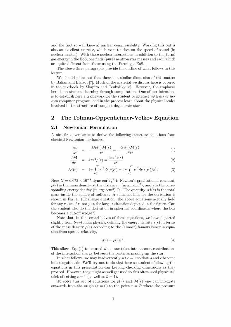
Here G = 6.673 × 10−8 dyne-cm2/g2 is Newton’s gravitational constant,ρ(r) is the mass density at the distance r (in gm/cm3), and ε is the corre-sponding energy density (in ergs/cm3) [9]. The quantity M(r) is the totalmass inside the sphere of radius r. A sufficient hint for the derivation isshown in Fig. 1. (Challenge question: the above equations actually holdfor any value of r, not just the large-r situation depicted in the figure. Canthe student also do the derivation in spherical coordinates where the boxbecomes a cut-off wedge?)

Note that, in the second halves of these equations, we have departedslightly from Newtonian physics, defining the energy density ε(r) in termsof the mass density ρ(r) according to the (almost) famous Einstein equa-tion from special relativity,

ε(r) = ρ(r)c2 . (4)

This allows Eq. (1) to be used when one takes into account contributionsof the interaction energy between the particles making up the star.

In what follows, we may inadvertently set c = 1 so that ρ and ε becomeindistinguishable. We’ll try not to do that here so students following theequations in this presentation can keeping checking dimensions as theyproceed. However, they might as well get used to this often-used physicists’trick of setting c = 1 (as well as h = 1).

To solve this set of equations for p(r) and M(r) one can integrateoutwards from the origin (r = 0) to the point r = R where the pressure

1

drA

p(r+dr) = F(r+dr)/A

p(r) = F(r)/A

Figure 1: Diagram for derivation of Eq. (1)

goes to zero. This point defines R as the radius of the star. One needs aninitial value of the pressure at r = 0, call it p0, to do this, and R and thetotal mass of the star, M(R) ≡ M , will depend on the value of p0.

Of course, to be able to perform the integration, one also needs to knowthe energy density ε(r) in terms of the pressure p(r). This relationship isthe equation of state (EoS) for the matter making up the star. Thus, alot of the student’s effort in this project will necessarily be directed todeveloping an appropriate EoS for the problem at hand.

2.2 General Relativistic Corrections

The Newtonian formulation presented above works well in regimes wherethe mass of the star is not so large that it significantly “warps” space-time. That is, integrating Eqs. (1) and (2) will work well in cases whengeneral relativistic (GR) effects are not important, such as for the compactstars known as white dwarfs. By creating a quantity using G that hasdimensions of length, the student can see when it becomes important toinclude GR effects. (This happens when GM/c2R becomes non-negligible.)As the student will see, this is the case for typical neutron stars.

It is probably not to be expected that an undergraduate physics majorderive the GR corrections to the above equations. For that, one can look atvarious textbook derivations of the Tolman-Oppenheimer-Volkov (TOV)equation [5] [8]. It should suffice to simply state the corrections to Eq. (1)in terms of three additional (dimensionless) factors,

dp

dr= −Gε(r)M(r)

c2r2

[

1 +p(r)

ε(r)

] [

1 +4πr3p(r)

M(r)c2

] [

1 − 2GM(r)

c2r

]−1

. (5)

The differential equation for M(r) remains unchanged. The first two fac-

2

tors in square brackets represent special relativity corrections of orderv2/c2. This can be seen in that pressure p goes, in the non-relativisticlimit, like k2

F /2m = mv2/2 (see Eq. (14) below) while ε and Mc2 go likemc2. That is, these factors reduce to 1 in the non-relativistic limit. (Thestudent should have, by now, realized that p and ε have the same dimen-sions.) The last factor is a GR correction and the size of GM/c2r, as weemphasized above, determines whether it is important (or not).

Note that the correction factors are all positive definite. It is as if New-tonian gravity becomes stronger at every r. That is, special and generalrelativity strengthens the relentless pull of gravity!

The coupled non-linear equations for p(r) and M(r) can also in thiscase be integrated from r = 0 for a starting value of p0 to the point wherep(R) = 0, to determine the star mass M = M(R) and radius R for thisvalue of p0. These equations invoke a balance between gravitational forcesand the internal pressure. The pressure is a function of the EoS, and forcertain conditions it may not be sufficient to withstand the gravitationalattraction. Thus the structure equations imply there is a maximum massthat a star can have.

2.3 White Dwarf Stars

2.3.1 A Few Facts

Let us violate (in words only) the second law of thermodynamics by warm-ing up on cold compact stars called white dwarfs. For these stellar objects,it suffices to solve the Newtonian structure equations, Eqs. (1)-(3) [10].

White dwarf stars [11] were first observed in 1844 by Friedrich Bessel(the same person who invented the special functions bearing that name).He noticed that the bright star Sirius wobbled back and forth and thendeduced that the visible star was being orbited by some unseen object, i.e.,it is a binary system. The object itself was resolved optically some 20 yearslater and thus earned the name of “white dwarf.” Since then numerousother white (and the smaller brown) dwarf stars have been observed (ordetected).

A white dwarf star is a low- or medium-mass star near the end of itslifetime, having burned up, through nuclear processes, most of its hydrogenand helium forming carbon, silicon or (perhaps) iron. They typically havea mass less than 1.4 times that of our Sun, M� = 1.989×1033 g [12]. Theyare also much smaller than our Sun, with radii of the order of 104 km (tobe compared with R� = 6.96× 105 km). These values can be worked outfrom the period of the wobble for the dwarf-normal star binary in the usualKeplerian way. As a result (and as is also the case for neutron stars), thenatural dimensions for discussing white dwarfs are for masses to be in unitsof solar mass, M�, and distances to be in km. Using these numbers thestudent should be able to make a quick estimate of the (average) densitiesof our Sun and of a white dwarf, to get a feel for the numbers that he willbe encountering.

Since GM/c2R ≈ 10−4 for such a typical white dwarf, we can concen-trate here on solving the non-relativistic structure equations of Sec. 2.1.(Question: why is it a good approximation to drop the special relativisticcorrections for these dwarfs?)

The reason a dwarf star is small is because, having burned up all thenuclear fuel it can, there is no longer enough thermal pressure to prevent

3

its gravity from crushing it down. As the density increases, the electronsin the atoms are pushed closer together, which then tend to fall into thelowest energy levels available to them. (The star begins to get colder.)Eventually the Pauli principle takes over, and the electron degeneracypressure (to be discussed next) provides the means for stabilizing the staragainst its gravitational attraction [12, 8]. This is the physics behindthe EoS which one needs to integrate the Newtonian structure equationsabove, Eqs. (1) and (2).

2.3.2 Fermi Gas Model for Electrons

For free electrons the number of states dn available at momentum k perunit volume is

dn =d3k

(2πh)3=

4πk2dk

(2πh)3. (6)

(This is a result from their modern physics course that students should re-view if they don’t remember it.) Integrating, one gets the electron numberdensity

n =8π

(2πh)3

∫ kF

0

k2dk =k3

F

3π2h3 . (7)

The additional factor of two comes in because there are two spin states foreach electron energy level. Here kF c, the Fermi energy, is the maximumenergy electrons can have in the star under consideration. It is a parameterwhich varies according to the star’s total mass and its history, but whichthe student is free to set in the calculations he or she is about to make.

Each electron is neutralized by a proton, which in turn is accompaniedin its atomic nucleus by a neutron (or perhaps a few more, as in the case ofa nucleus like 56Fe26). Thus, neglecting the electron mass me with respectto the nucleon mass mN , the mass density of the star is essentially givenby

ρ = nmNA/Z , (8)

where A/Z is the number of nucleons per electron. For 12C, A/Z = 2.00,while for 56Fe, A/Z = 2.15 . Note that, since n is a function of kF , so isρ. Conversely, given a value of ρ,

kF = h

(

3π2ρ

mN

Z

A

)1/3

. (9)

The energy density of this star is also dominated by the nucleon masses,i.e., ε ≈ ρc2.

The contribution to the energy density from the electrons (includingtheir rest masses) is

εelec(kF ) =8π

(2πh)3

∫ kF

0

(k2c2 + m2ec

4)1/2k2dk

= ε0

∫ kF /mec

0

(u2 + 1)1/2u2du

=ε08

[

(2x3 + x)(1 + x2)1/2 − sinh−1(x)]

, (10)

where

ε0 =m4

ec5

π2h3 (11)

4

carries the desired dimensions of energy per volume and x = kF /mec. Thetotal energy density is then

ε = nmNA/Z + εelec(kF ) . (12)

One should check that the first term here is much larger than the second.To get our desired EoS, we need an expression for the pressure. The fol-

lowing presents a problem (!) that the student should work through. Fromthe first law of thermodynamics, dU = dQ − pdV , then at temperature Tfixed at T = 0 (where dQ = 0 since dT = 0)

p = − ∂U

∂V

]

T=0

= n2 d(ε/n)

dn= n

dε

dn− ε = nµ − ε , (13)

where the energy density here is the total one given by Eq. (12). Thequantity µi = dε/dni defined in the last equality is known as the chemicalpotential of the electrons. This is a concept which will be especially usefulin Section 5 where we consider an equilibrium mix of neutrons, protonsand electrons.

Utilizing Eq. (10), Eq. (13) yields the pressure (another problem!)

p(kF ) =8π

3(2πh)3

∫ kF

0

(k2c2 + m2ec

4)−1/2k4dk

=ε03

∫ kF /mec

0

(u2 + 1)−1/2u4du

=ε024

[

(2x3 − 3x)(1 + x2)1/2 + 3 sinh−1(x)]

. (14)

(Hint: use the n2d(ε/n)/dn form and remember to integrate by parts.)Using Mathematica [13] the student can show that the constant ε0 =

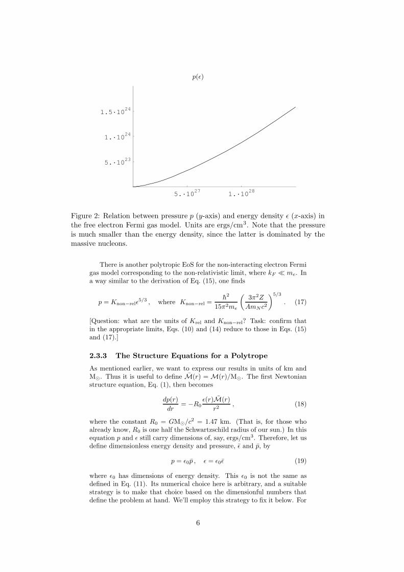
1.42×1024 in units that, at this point, are erg/cm3. (Yet another problem:verify that the units of ε0 are as claimed [14].) One also finds that Math-ematica can perform the integrals analytically. (We quoted the resultsalready in the equations above.) They are a bit messy, however, as theyboth involve an inverse hyperbolic sine function, and thus are not terriblyenlightening. It is useful, however, for the student to make a plot of ε ver-sus p (such as shown in Fig. 2) for values of the parameter 0 ≤ kF ≤ 2me.This curve has a shape much like ε4/3 (the student should compare withthis), and there is a good reason for that.

Consider the (relativistic) case when kF � me. Then Eq. (14) simpli-fies to

p(kF ) =ε03

∫ kF /mec

0

u3du =ε012

(kF /mec)4 =

hc

12π2

(

3π2Zρ

mNA

)4/3

≈ Krel ε4/3 , (15)

where

Krel =hc

12π2

(

3π2Z

AmNc2

)4/3

. (16)

A star having simple EoS like p = Kεγ is called a “polytrope”, and wetherefore see that the relativistic electron Fermi gas gives a polytropic EoSwith γ = 4/3. As will be seen in the next subsection, a polytropic EoSallows one to solve the structure equations (numerically) in a relativelystraight-forward way [15].

5

p(ε)

5.·1027 1.·1028

5.·1023

1.·1024

1.5·1024

Figure 2: Relation between pressure p (y-axis) and energy density ε (x-axis) inthe free electron Fermi gas model. Units are ergs/cm3. Note that the pressureis much smaller than the energy density, since the latter is dominated by themassive nucleons.

There is another polytropic EoS for the non-interacting electron Fermigas model corresponding to the non-relativistic limit, where kF � me. Ina way similar to the derivation of Eq. (15), one finds

p = Knon−relε5/3 , where Knon−rel =

h2

15π2me

(

3π2Z

AmNc2

)5/3

. (17)

[Question: what are the units of Krel and Knon−rel? Task: confirm thatin the appropriate limits, Eqs. (10) and (14) reduce to those in Eqs. (15)and (17).]

2.3.3 The Structure Equations for a Polytrope

As mentioned earlier, we want to express our results in units of km andM�. Thus it is useful to define M(r) = M(r)/M�. The first Newtonianstructure equation, Eq. (1), then becomes

dp(r)

dr= −R0

ε(r)M(r)

r2, (18)

where the constant R0 = GM�/c2 = 1.47 km. (That is, for those whoalready know, R0 is one half the Schwartzschild radius of our sun.) In thisequation p and ε still carry dimensions of, say, ergs/cm3. Therefore, let usdefine dimensionless energy density and pressure, ε and p, by

p = ε0p , ε = ε0ε (19)

where ε0 has dimensions of energy density. This ε0 is not the same asdefined in Eq. (11). Its numerical choice here is arbitrary, and a suitablestrategy is to make that choice based on the dimensionful numbers thatdefine the problem at hand. We’ll employ this strategy to fix it below. For

6

a polytrope, we can write

p = Kε γ , where K = Kε γ−10 is dimensionless. (20)

It is easier to solve Eq. (18) for p, so we should express ε in terms of it,

ε = (p/K)1/γ . (21)

Equation (18) can now be recast in the form

dp(r)

dr= −α p(r)1/γM(r)

r2, (22)

where the constant α is

α = R0/K1/γ = R0/(Kεγ−10 )1/γ . (23)

Equation (22) has dimensions of 1/km, with α in km (since R0 is). Thatis, it is to be integrated with respect to r, with r also in km.

We can choose any convenient value for α since ε0 is still free. For agiven value of α, ε0 is then fixed at

ε0 =

[

1

K

(

R0

α

)γ]1−γ

. (24)

We also need to cast the other coupled equation, Eq. (2), in terms ofdimensionless p and M,

dM(r)

dr= βr2p(r)1/γ , (25)

where [16]

β =4πε0

M�c2K1/γ=

4πε0

M�c2(Kεγ−10 )1/γ

. (26)

Equation (25) also carries dimensions of 1/km, the constant β havingdimesnions 1/km3. Note that, in integrating out from r = 0, the initialvalue of M(0) = 0.

2.3.4 Integrating the Polytrope Numerically

Our task is to integrate the coupled first-order differential equations (DE),Eqs. (22) and (25), out from the origin, r = 0, to the point R where thepressure falls to zero, p(R) = 0 [17]. To do this we need two initial values,p(0) (which must be positive) and M(0) ( which we already know mustbe 0). The star’s radius, R, and its mass M = M(R) in units of M� willvary, depending on the choice for p(0).

For purposes of numerical stability in solving Eqs. (22) and (25), wewant the constants α and β to be not much different from each other (andprobably not much different from 1). We will see below that this can bearranged for both of the two polytropic EoS’s discussed above for whitedwarfs.

Our coupled DE’s are quite non-linear. In fact, because of the p1/γ

factors, the solution will become complex when p(r) < 0, i.e., when r > R.Thus we will want to recognize when this happens. How can this beprogrammed?

7

Mathematica and similar symbolic/numerical packages have built-infirst-order DE solvers. Perhaps the solver is as simple as a fixed, equal-step Runge-Kutta routine (as in MathCad 7 Standard), but there are oftenmore sophisticated solvers in more recent versions. These packages alsoallow for program control constructs such as do-loops, whiles and the like.

Thus, consider a do-loop on a variable r running in appropriately smallsteps over a range that is sure to contain the expected value of R. Callthe DE solver inside this loop, integrating the coupled DE’s from r = 0 tor. When the solver routine exits, check to see if the last value of p, i.e.,p(r), has a real part which has gone negative. If so, then break out of theloop, calling R = r. If not, go on to the next larger value of r and call theDE solver again.

More discussion of how to program the integration of the DE’s is in-appropriate here, since we want to encourage the student to learn fromprogramming to appreciate how the symbolic/numerical package is used.

2.3.5 The Relativistic Case kF � me

This is the regime for white dwarfs with the largest mass. A larger massneeds a greater central pressure to support it. However, large centralpressures mean the squeezed electrons become relativistic.

Recall that the polytrope exponent γ = 4/3 for this case and theequation of state is given by P = Krelε

γ with Krel given by Eq. (16).After some trial and error, we chose in our program (the student maywant to try something else)

α = R0 = 1.473 km [kF � me] , (27)

which in turn fixes, from Eq. (24),

ε0 = 7.463× 1039ergs/cm3 = 4.17 M�c2/km3 [kF � me] . (28)

The first question the student should ask, in checking this number, iswhether such a large number is physically reasonable.

Continuing with the kF � me numerics, Eqs. (16) and (26) give

β = 52.46 /km3 [kF � me] , (29)

which is about 30 times larger than α, but probably manageable from thestandpoint of performing the numerical integration.

In our first attempt to integrate the coupled DE’s for this case (usinga do-loop as described above) we chose p(0) = 1.0. This gives us a whitedwarf of radius R ≈ 2 km, which is miniscule compared with the expectedradius of ≈ 104 km! Why? What went wrong?

The student who also makes this kind of mistake will eventually realizethat our choice of scale, ε0 = 4.17M�c2/km3, represents a huge energydensity. One can simply estimate the average energy density of a starwith a 104 km radius and a mass of one solar mass by the ratio of its restmass energy to its volume,

〈ε〉 ≈ M�c2

R3= 10−12 M�c2/km3 , (30)

which is much, much smaller than the ε0 here. In addition, the pressure pis about 2000 times smaller than the energy density ε (see Fig. 2). Thus,choosing a starting value of p(0) ∼ 10−15 would probably be more physical.

8

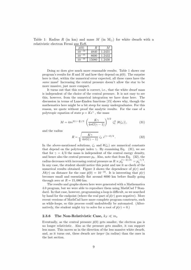
Table 1: Radius R (in km) and mass M (in M�) for white dwarfs with arelativistic electron Fermi gas EoS.

p(0) R M10−14 4840 1.243110−15 8600 1.243210−16 15080 1.2430

Doing so does give much more reasonable results. Table 1 shows ourprogram’s results for R and M and how they depend on p(0). The surprisehere is that, within the numerical error expected, all these cases have thesame mass! Increasing the central pressure doesn’t allow the star to bemore massive, just more compact.

It turns out that this result is correct, i.e., that the white dwarf massis independent of the choice of the central pressure. It is not easy to seethis, however, from the numerical integration we have done here. Thediscussion in terms of Lane-Emden functions [15] shows why, though themathematics here might be a bit steep for many undergraduates. For thisreason, we quote without proof the analytic results. For the case of apolytropic equation of state p = Kεγ , the mass

M = 4πε2(γ−4

3)/3

(

Kγ

4πG(γ − 1)

)3/2

ζ21 |θ(ζ1)| , (31)

and the radius

R =

√

Kγ

4πG(γ − 1)ζ1 ε(γ−2)/2 . (32)

In the above-mentioned solutions, ζ1 and θ(ζ1) are numerical constantsthat depend on the polytropic index γ. By examining Eq. (31), we seethat for γ = 4/3 the mass is independent of the central energy density,and hence also the central pressure p0. Also, note that from Eq. (32), the

radius decreases with increasing central pressure as R ∝ p(γ−2)/2γ0 = p

−1/40 .

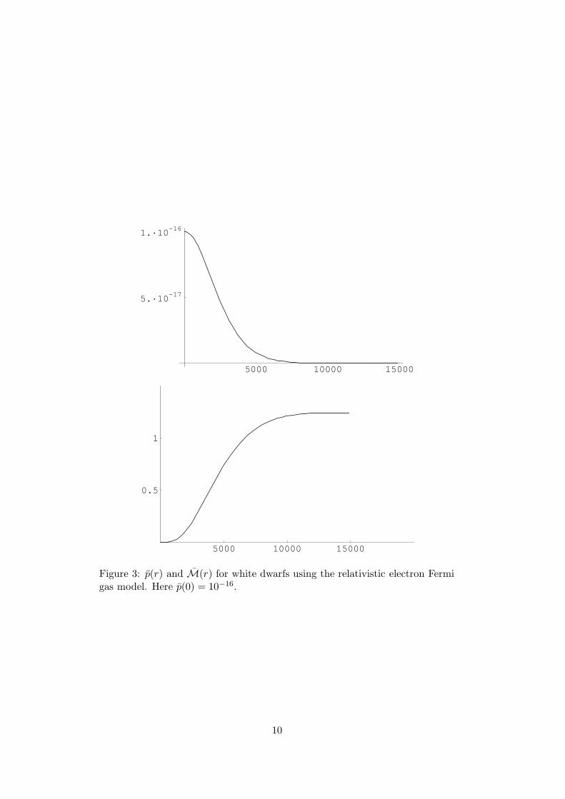
In any case, the student should notice this point and use it as check of thenumerical results obtained. Figure 3 shows the dependence of p(r) andM(r) on distance for the case p(0) = 10−16. It is interesting that p(r)becomes small and essentially flat around 8000 km before finally goingthrough zero at R = 15, 080 km.

The results and graphs shown here were generated with a Mathematica4.0 program, but we were able to reproduce them using MathCad 7 Stan-dard. In that case, however, programming a loop is difficult, so we searchedby hand for the endpoint (where the real part of p(r) goes negative). Morerecent versions of MathCad have more complete program constructs, suchas while-loops, so this process could undoubtedly be automated. (Alter-natively, the student might try to solve for a root of p(r) = 0.)

2.3.6 The Non-Relativistic Case, kF � me

Eventually, as the central pressure p(0) gets smaller, the electron gas isno longer relativistic. Also as the pressure gets smaller, it can supportless mass. This moves us in the direction of the less massive white dwarfs,and, as it turns out, these dwarfs are larger (in radius) than the ones inthe last section.

9

5000 10000 15000

5.·10-17

1.·10-16

5000 10000 15000

0.5

1

Figure 3: p(r) and M(r) for white dwarfs using the relativistic electron Fermigas model. Here p(0) = 10−16.

10

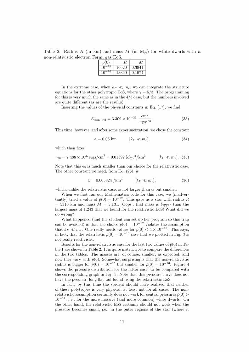
Table 2: Radius R (in km) and mass M (in M�) for white dwarfs with anon-relativistic electron Fermi gas EoS.

p(0) R M10−15 10620 0.394110−16 13360 0.1974

In the extreme case, when kF � me, we can integrate the structureequations for the other polytropic EoS, where γ = 5/3. The programmingfor this is very much the same as in the 4/3 case, but the numbers involvedare quite different (as are the results).

Inserting the values of the physical constants in Eq. (17), we find

Knon−rel = 3.309× 10−23 cm2

ergs2/3. (33)

This time, however, and after some experimentation, we chose the constant

α = 0.05 km [kF � me] , (34)

which then fixes

ε0 = 2.488× 1037ergs/cm3

= 0.01392 M�c2/km3 [kF � me] . (35)

Note that this ε0 is much smaller than our choice for the relativistic case.The other constant we need, from Eq. (26), is

β = 0.005924 /km3 [kF � me] , (36)

which, unlike the relativistic case, is not larger than α but smaller.When we first ran our Mathematica code for this case, we (inadver-

tantly) tried a value of p(0) = 10−12. This gave us a star with radius R= 5310 km and mass M = 3.131. Oops!, that mass is bigger than thelargest mass of 1.243 that we found for the relativistic EoS! What did wedo wrong?

What happened (and the student can set up her program so this trapcan be avoided) is that the choice p(0) = 10−12 violates the assumptionthat kF � me. One really needs values for p(0) < 4 × 10−15. This says,in fact, that the relativistic p(0) = 10−16 case that we plotted in Fig. 3 isnot really relativistic.

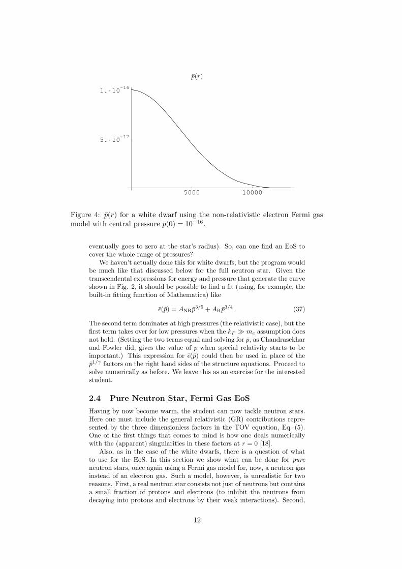
Results for the non-relativistic case for the last two values of p(0) in Ta-ble 1 are shown in Table 2. It is quite instructive to compare the differencesin the two tables. The masses are, of course, smaller, as expected, andnow they vary with p(0). Somewhat surprising is that the non-relativisticradius is bigger for p(0) = 10−15 but smaller for p(0) = 10−16. Figure 4shows the pressure distribution for the latter case, to be compared withthe corresponding graph in Fig. 3. Note that this pressure curve does nothave the peculiar, long flat tail found using the relativistic EoS.

In fact, by this time the student should have realized that neitherof these polytropes is very physical, at least not for all cases. The non-relativistic assumption certainly does not work for central pressures p(0) >10−14, i.e., for the more massive (and more common) white dwarfs. Onthe other hand, the relativistic EoS certainly should not work when thepressure becomes small, i.e., in the outer regions of the star (where it

11

p(r)

5000 10000

5.·10-17

1.·10-16

Figure 4: p(r) for a white dwarf using the non-relativistic electron Fermi gasmodel with central pressure p(0) = 10−16.

eventually goes to zero at the star’s radius). So, can one find an EoS tocover the whole range of pressures?

We haven’t actually done this for white dwarfs, but the program wouldbe much like that discussed below for the full neutron star. Given thetranscendental expressions for energy and pressure that generate the curveshown in Fig. 2, it should be possible to find a fit (using, for example, thebuilt-in fitting function of Mathematica) like

ε(p) = ANRp3/5 + ARp3/4 . (37)

The second term dominates at high pressures (the relativistic case), but thefirst term takes over for low pressures when the kF � me assumption doesnot hold. (Setting the two terms equal and solving for p, as Chandrasekharand Fowler did, gives the value of p when special relativity starts to beimportant.) This expression for ε(p) could then be used in place of thep1/γ factors on the right hand sides of the structure equations. Proceed tosolve numerically as before. We leave this as an exercise for the interestedstudent.

2.4 Pure Neutron Star, Fermi Gas EoS

Having by now become warm, the student can now tackle neutron stars.Here one must include the general relativistic (GR) contributions repre-sented by the three dimensionless factors in the TOV equation, Eq. (5).One of the first things that comes to mind is how one deals numericallywith the (apparent) singularities in these factors at r = 0 [18].

Also, as in the case of the white dwarfs, there is a question of whatto use for the EoS. In this section we show what can be done for pure

neutron stars, once again using a Fermi gas model for, now, a neutron gasinstead of an electron gas. Such a model, however, is unrealistic for tworeasons. First, a real neutron star consists not just of neutrons but containsa small fraction of protons and electrons (to inhibit the neutrons fromdecaying into protons and electrons by their weak interactions). Second,

12

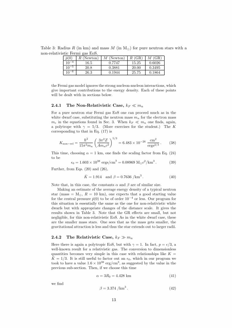
Table 3: Radius R (in km) and mass M (in M�) for pure neutron stars with anon-relativistic Fermi gas EoS.

p(0) R (Newton) M (Newton) R (GR) M (GR)10−4 16.5 0.7747 15.25 0.602610−5 20.8 0.3881 20.00 0.349510−6 26.3 0.1944 25.75 0.1864

the Fermi gas model ignores the strong nucleon-nucleon interactions, whichgive important contributions to the energy density. Each of these pointswill be dealt with in sections below.

2.4.1 The Non-Relativistic Case, kF � mn

For a pure neutron star Fermi gas EoS one can proceed much as in thewhite dwarf case, substituting the neutron mass mn for the electron massme in the equations found in Sec. 3. When kF � mn one finds, again,a polytrope with γ = 5/3. (More exercises for the student.) The Kcorresponding to that in Eq. (17) is

Knon−rel =h2

15π2mn

(

3π2Z

Amnc2

)5/3

= 6.483× 10−26 cm2

ergs2/3. (38)

This time, choosing α = 1 km, one finds the scaling factor from Eq. (24)to be

ε0 = 1.603× 1038 ergs/cm3

= 0.08969 M�c2/km3 . (39)

Further, from Eqs. (20) and (26),

K = 1.914 and β = 0.7636 /km3 . (40)

Note that, in this case, the constants α and β are of similar size.Making an estimate of the average energy density of a typical neutron

star (mass = M�, R = 10 km), one expects that a good starting valuefor the central pressure p(0) to be of order 10−4 or less. Our program forthis situation is essentially the same as the one for non-relativistic whitedwarfs but with appropriate changes of the distance scale. It gives theresults shown in Table 3. Note that the GR effects are small, but notnegligible, for this non-relativistic EoS. As in the white dwarf case, theseare the smaller mass stars. One sees that as the mass gets smaller, thegravitational attraction is less and thus the star extends out to larger radii.

2.4.2 The Relativistic Case, kF � mn

Here there is again a polytropic EoS, but with γ = 1. In fact, p = ε/3, awell-known result for a relativistic gas. The conversion to dimensionlessquantities becomes very simple in this case with relationships like K =K = 1/3. It is still useful to factor out an ε0, which in our program wetook to have a value 1.6 × 1038 erg/cm3, as suggested by the value in theprevious sub-section. Then, if we choose this time

α = 3R0 = 4.428 km (41)

we findβ = 3.374 /km3 . (42)

13

We expect central pressures p(0) in this case to be greater than 10−4.Other than these changes, we wrote a similar program to the one above,taking care to avoid exponents like 1/(γ − 1).

Running that code gives, at first glance, enormous radii, values of Rgreater than 50 km! We can imagine the student looking frantically fora program bug that isn’t there. In fact, what really happens is that, forthis EoS, the loop on r runs through its whole range, since the pressurep(r) never passes through zero. (A plot of p(r) looks quite similar, butfor distance scale, to that shown in Fig. 3, where γ = 4/5.) It only fallsmonotonically toward zero, getting ever smaller. By the time the studentrecognizes this, she will probably also have realized that the relativistic gasEoS is inappropriate for such small pressures. Something better should bedone (as in the next sub-section).

It turns out that the structure equations for γ = 1 are sufficientlysimple that an analytic solution for p(r) can be found, which corroboratesthe above remarks about not having a zero at a finite R. A suggestion forthe student is to try a power-law Ansatz.

2.4.3 The Fermi Gas EoS for Arbitrary Relativity

In order to avoid the trap of the relativistic gas, one should find an EoSfor the non-interacting neutron Fermi gas which works for all values of therelativity parameter x = kF /mnc. Taking a hint from the two polytropes,one can try to fit the energy density as a function of pressure, each givenas a transcendental function of kF , with the form

ε(p) = ANRp3/5 + ARp . (43)

For low pressures the non-relativistic first term dominates over the second.(The power in the relativistic term is changed from that in Eq. (37).) It isagain useful to factor out an ε0 from both ε and p. In this case, it is morenatural to define it as

ε0 =m4

nc5

(3π2h)3= 5.346× 1036 ergs

cm3= 0.003006

M�c2

km3 . (44)

Mathematica can easily create a table of exact ε and p values as afunction of kF . The dimensionless A-values can then be fit using its built-in fitting function. From our efforts we found, to an accuracy of betterthan 1% over most of the range of kF [19],

ANR = 2.4216 , AR = 2.8663 . (45)

We used the fitted functional form for ε of Eq. (43) in a Mathematicaprogram similar to that for the neutron star based on the non-relativisticEoS. With the ε0 of Eq. (44) and choosing α = R0 = 1.476 km, we obtainβ = 0.03778. Our results for a starting value of p(0) = 0.01, clearly in therelativistic regime, are

R = 15.0 , M = 1.037 , Newtonian equations (46)

R = 13.4 , M = 0.717 , full TOV equation . (47)

For this more massive star, the GR effects are significant (as should beexpected from the size of GM/c2R, about 10% in this case). Figure 5displays the differences.

14

2 4 6 8 10 12r

0.002

0.004

0.006

0.008

0.01

2 4 6 8 10 12r

0.2

0.4

0.6

0.8

1

Figure 5: p(r) and M(r) (r in km) for a pure neutron star with central pressurep(0) = 0.01, using a Fermi gas EoS fit valid for all values of kF . The thin curvesare results from the classical Newtonian structure equations, while the thickones include general relativistic corrections.

15

M(R)

5 10 15 20 25

0.2

0.4

0.6

0.8

1

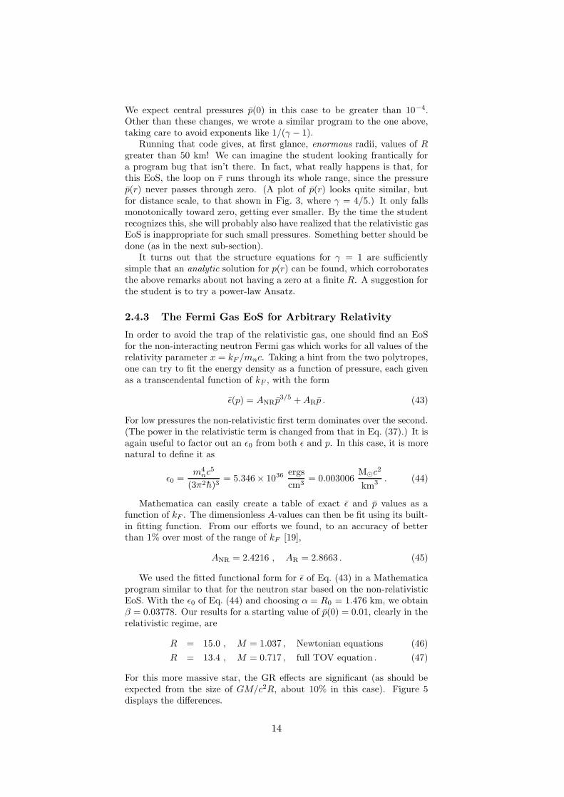
Figure 6: The mass M (in M�) and radius R (in km) for pure neutron stars,using a Fermi gas EoS. The stars of low mass and large radius are solutions ofthe TOV equations for small values of central pressure p(0). The stars to theright of the maximum at R = 11 are stable, while those to the left will suffergravitational collapse.

It is now instructive to make a long run of calculations for a range ofp(0) values. We display in Fig. 6 a (parametric) plot of M and R as theydepend on the central pressure. The low-mass/large-radius stars are tothe right in the graph and correspond to small starting values of p(0). Asthe central pressure increases, the total mass that the star can supportincreases. And, the bigger the star mass, the bigger the gravitationalattraction which draws in the periphery of the star, making stars withsmaller radii. That is, increasing p(0) corresponds to “climbing the hill,”moving upward and to the left in the diagram.

At about p(0) = 0.03 one gets to the top of the hill, achieving a max-imum mass of about 0.8 M� at a radius R ≈ 11 km. That maximum Mand its R agree with Oppenheimer and Volkov’s seminal 1939 result for aFermi gas EoS.

What about the solutions in Fig. 6 that are “over the hill,” i.e., to theleft of the maximum? It turns out that these stars are unstable againstgravitational collapse into a black hole. The question of stability, however,is a complicated issue [20], perhaps too difficult for a student at this level.The fact that things collapse to the left of the maximum, however, meansthat one probably shouldn’t worry too much about the peculiar curly-cue tail to the M -R curve in the figure. It appears to be an artifact forvery large values of p(0), also seen in other calculations, even though it isespecially prominent for this Fermi gas EoS.

2.4.4 Why Is There a Maximum Mass?

On general grounds one can argue that cold compact objects such as whitedwarfs and neutron stars must possess a limiting mass beyond which stablehydrostatic configurations are not possible. This limiting mass is oftencalled the maximum mass of the object and was briefly mentioned in the

16

discussion at the end of Sec. 2.2 and that relating to Fig. 6. In whatfollows, we outline the general argument.

The thermal component of the pressure in cold stars is by definitionnegligible. Thus, variations in both the energy density and pressure areonly caused by changes in the density. Given this simple observation, letus examine why we expect a maximum mass in the Newtonian case.

Here, an increase in the density results in a proportional increase in theenergy density. This results in a corresponding increase in the gravitationalattraction. To balance this, we require that the increment in pressure islarge enough. However, the rate of change of pressure with respect toenergy density is related to the speed of sound (see Sec. 6.3). In a purelyNewtonian world, this is in principle unbounded. However, the speed ofall propagating signals cannot exceed the speed of light. This then puts abound on the pressure increment associated with changes in density.

Once we accept this bound, we can safely conclude that all cold com-pact objects will eventually run into the situation in which any increase indensity will result in an additional gravitational attraction that cannot becompensated for by the corresponding increment in pressure. This leadsnaturally to the existence of a limiting mass for the star.

When we include general relativistic corrections, as discussed in Sec. 2.2earlier, they act to “amplify” gravity. Thus we can expect the maximummass to occur at a somewhat lower mass than in the Newtonian case.

2.5 Neutron Stars with Protons and Electrons, Fermi

Gas EoS

As mentioned at the beginning of the last section, neutron stars are notmade only of neutrons. There must also be a small fraction of protons andelectrons present. The reason for this is that a free neutron will undergoa weak decay,

n → p + e− + νe , (48)

with a lifetime of about 15 minutes. So, there must be something thatprevents this decay in the case of the star, and that is the presence of theprotons and electrons.

The decay products have low energies (mn − mp − me = 0.778 MeV),with most of that energy being carried away by the light electron and(nearly massless) neutrino [21]. If all the available low-energy levels forthe decay proton are already filled by the protons already present, thenthe Pauli exclusion principle takes over and prevents the decay from takingplace.

The same might be said about the presence of the electrons, but in anycase the electrons must be present within the star to cancel the positivecharge of the protons. A neutron star is electrically neutral. We sawearlier that the number density of a particle species is fixed in terms ofthat particle’s Fermi momentum [see Eq. (7)]. Thus equal numbers ofelectrons and protons implies that

kF,p = kF,e . (49)

In addition to charge neutrality, we also require weak interaction equi-librium, i.e., as many neutron decays [Eq. (48)] taking place as electroncapture reactions, p + e− → n + νe. This equilibrium can be expressed in

17

terms of the chemical potentials for the three particle species,

µn = µp + µe . (50)

We already defined the chemical equilibrium for a particle in Sec. 3.2 afterEq. (13),

µi(kF,i) =dε

dn= (k2

F,i + m2i )

1/2 , i = n, p, e . (51)

where, for the time being, we have set c = 1 to simplify the equationssomewhat. (The student is urged to prove the right-hand equality.) FromEqs. (49), (50), and (51) we can find a constraint determining kF,p for agiven kF,n,

(k2F,n + m2

n)1/2 − (k2F,p + m2

p)1/2 − (k2

F,p + m2e)

1/2 = 0 . (52)

While an ambitious algebraist can probably solve this equation for kF,p

as a function of kF,n, we were somewhat lazy and let Mathematica do it,finding

kF,p(kF,n) =[(k2

F,n + m2n − m2

e)2 − 2m2

p(k2F,n + m2

n + m2e) + m4

p]1/2

2(k2F,n + m2

n)1/2(53)

≈k2

F,n + m2n − m2

p

2(k2F,n + m2

n)1/2for

me

kF,n→ 0 . (54)

The total energy density is the sum of the individual energy densities,

εtot =∑

i=n,p,e

εi , (55)

where

εi(kF,i) =

∫ kF,i

0

(k2 + mi)1/2k2dk = ε0 εi(xi, yi) , (56)

and, as before [22],

ε0 = m4n/3π2h3 , (57)

εi(xi, yi) =

∫ xi

0

(u2 + y2i )1/2u2du , (58)

xi = kF,i/mi , yi = mi/mn . (59)

The corresponding total pressure is

ptot =∑

i=n,p,e

pi , (60)

pi(kF,i) =

∫ kF,i

0

(k2 + mi)−1/2k4dk = ε0 pi(xi, yi) , (61)

pi(xi, yi) =

∫ xi

0

(u2 + y2i )−1/2u4du . (62)

Using Mathematica the (dimensionless) integrals can be expressed interms of log and sinh−1 functions of xi and yi. One can then generate atable of εtot versus ptot values for an appropriate range of kF,n’s. This, inturn, can be fitted to the same form of two terms as before in Eq. (43).We found, this time, the coefficients to be

ANR = 2.572 , AR = 2.891 . (63)

18

These coefficients are not much changed from those in Eq. (45) for thepure neutron star. Therefore, we expect that the M versus R diagram forthis more realistic Fermi gas model would not be much different from thatin Fig. 6.

2.6 Introducing Nuclear Interactions

Nucleon-nucleon interactions can be included in the EoS (they are im-portant) by constructing a simple model for the nuclear potential thatreproduces the general features of (normal) nuclear matter. In doing sowe were much guided by the lectures of Prakash [6].

We will use MeV and fm (10−13 cm) as our energy and distance unitsfor much of this section, converting back to M� and km later. We willalso continue setting c = 1 for now. In this regard, the important numberto remember for making conversions is hc = 197.3 MeV-fm. We will alsoneglect the mass difference between protons and neutrons, labeling theirmasses as mN .

The Bethe-Weizacker mass formula [23] for the binding energy of nu-clides with Z protons and N neutrons (mass number A = N + Z) reads

BE = EVolA−ESurfA2/3 −ESym

(N − Z)2

A− 3

5

Z(Z − 1)e2

4πε0RA+EPair, (64)

where the volume contribution to the binding energy pro nucleon is thedominant one in the limit of infinite nuclear matter limA→∞ EVol = (E/A−mN )|n0

= 16 MeV. The suface energy is ESurf = 17 MeV, the symmetryenergy is ESym = 30 MeV and for the pairing energy there are three pos-sibilities EPair = {∆, 0,−∆} for {even-even, even-odd, odd-odd} nuclei,respectively. The pairing energy gap is ∆ = 25 A−1 MeV. The remainingterm in (64) is the Coulomb energy, which depends on the nuclear chargenumber Z and the nuclear radius RA = 1.24 A1/3 fm. For normal sym-metric nuclear matter (N = Z), an equilibrium number density n0 of 0.16nucleons/fm3 is obtained. For this value of n0 the Fermi momentum isk0

F = 263 MeV/c [see Eq. (7)]. This momentum is small enough comparedwith mN = 939 MeV/c2 to allow a non-relativistic treatment of normalnuclear matter. At this density, the average binding energy per nucleon,BE = E/A−mN , is −16 MeV. These are two physical quantities we def-initely want our nuclear potential to respect, but there are two more thatwe’ll need to fix the parameters of the model.

We chose one of these as the nuclear compressibility, K0, to be definedbelow. This is a quantity which is not all that well established but is inthe range of 200 to 400 MeV. The other is the so-called symmetry energy

term, which, when Z = 0, contributes about 30 MeV of energy above thesymmetric matter minimum at n0. (This quantity might really be betterdescribed as an asymmetry parameter, since it accounts for the energythat comes in when N 6= Z.)

2.6.1 Symmetric Nuclear Matter

We defer the case when N 6= Z, which is our main interest in this paper, tothe next sub-section. Here we concentrate on getting a good (enough) EoSfor nuclear matter when N = Z, or, equivalently, when the proton andneutron number densities are equal, nn = np. The total nucleon densityn = nn + np.

19

We need to relate the first three nuclear quantities, n0, BE, and K0

to the energy density for symmetric nuclear matter, ε(n). Here n = n(kF )is the nuclear density (at and away from n0). We will not worry in thissection about the electrons that are present, since, as was seen in the lastsection, its contribution is small. The energy density now will include thenuclear potential, V (n), which we will model below in terms of two simplefunctions with three parameters that are fitted to reproduce the abovethree nuclear quantities. [The fourth quantity, the symmetry energy, willbe used in the next sub-section to fix a term in the potential which isproportional to (N − Z)/A.]

First, the average energy per nucleon, E/A, for symmetric nuclearmatter is related to ε by

E(n)/A = ε(n)/n , (65)

which includes the rest mass energy, mN and has dimensions of MeV. Asa function of n, E(n)/A − mN has a minimum at n = n0 with a depthBE = −16 MeV. This minimum occurs when

d

dn

(

E(n)

A

)

=d

dn

(

ε(n)

n

)

= 0 at n = n0 . (66)

This is one constraint of the parameters of V (n). Another, of course, isthe binding energy,

ε(n)

n− mN = BE at n = n0 . (67)

The positive curvature at the bottom of this valley is related to the nuclear(in)compressibility by [24]

K(n) = 9dp(n)

dn= 9

[

n2 d2

dn2

( ε

n

)

+ 2nd

dn

( ε

n

)

]

, (68)

using Eq. (13), which defines the pressure in terms of the energy density.At n = n0 this quantity equals K0. (The factor of 9 is a historical artifactfrom the convention originally defining K0.)

(Question: why does one not have to calculate the pressure at n = n0?)The N = Z potential in ε(n) we will model as [6]

ε(n)

n= mN +

3

5

h2k2F

2mN+

A

2u +

B

σ + 1uσ , (69)

where u = n/n0 and σ are dimensionless and A and B have dimensions ofMeV. The first term represents the rest mass energy and the second theaverage kinetic energy per nucleon. [These two terms are leading in thenon-relativistic limit of the nucleonic version of Eq. (10).] For kF (n0) = k0

F

we will abbreviate the kinetic energy term as⟨

E0F

⟩

, which evaluates to22.1 MeV. The kinetic energy term in Eq. (69) can be better written as⟨

E0F

⟩

u2/3.From the above three constraints, Eqs. (66)-(68), and noting that u = 1

at n = n0, we get three equations for the parameters A, B, and σ:

⟨

E0F

⟩

+A

2+

B

σ + 1= BE , (70)

2

3

⟨

E0F

⟩

+A

2+

Bσ

σ + 1= 0 , (71)

10

9

⟨

E0F

⟩

+ A + Bσ =K0

9. (72)

20

E/A − mN

0.5 1 1.5 2u

-15

-10

-5

5

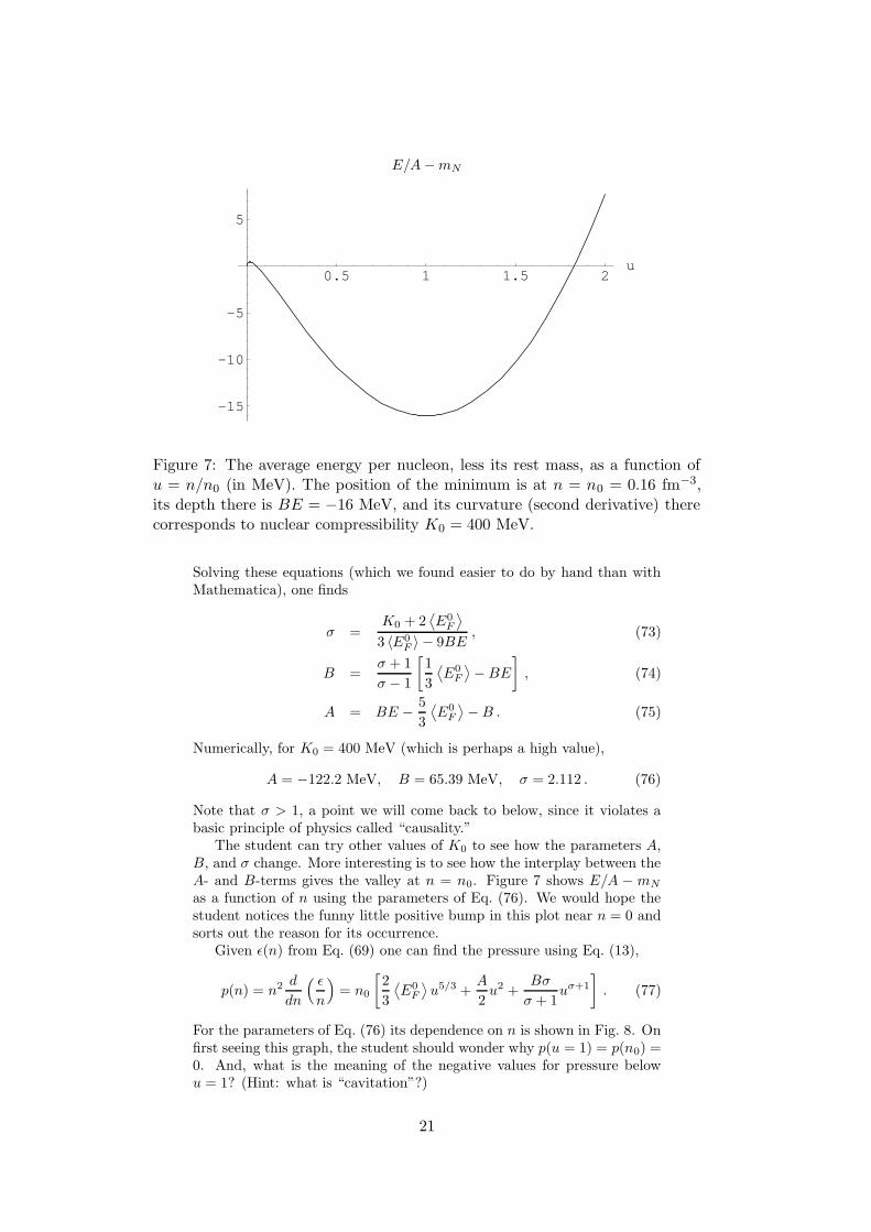
Figure 7: The average energy per nucleon, less its rest mass, as a function ofu = n/n0 (in MeV). The position of the minimum is at n = n0 = 0.16 fm−3,its depth there is BE = −16 MeV, and its curvature (second derivative) therecorresponds to nuclear compressibility K0 = 400 MeV.

Solving these equations (which we found easier to do by hand than withMathematica), one finds

σ =K0 + 2

⟨

E0F

⟩

3 〈E0F 〉 − 9BE

, (73)

B =σ + 1

σ − 1

[

1

3

⟨

E0F

⟩

− BE

]

, (74)

A = BE − 5

3

⟨

E0F

⟩

− B . (75)

Numerically, for K0 = 400 MeV (which is perhaps a high value),

A = −122.2 MeV, B = 65.39 MeV, σ = 2.112 . (76)

Note that σ > 1, a point we will come back to below, since it violates abasic principle of physics called “causality.”

The student can try other values of K0 to see how the parameters A,B, and σ change. More interesting is to see how the interplay between theA- and B-terms gives the valley at n = n0. Figure 7 shows E/A − mN

as a function of n using the parameters of Eq. (76). We would hope thestudent notices the funny little positive bump in this plot near n = 0 andsorts out the reason for its occurrence.

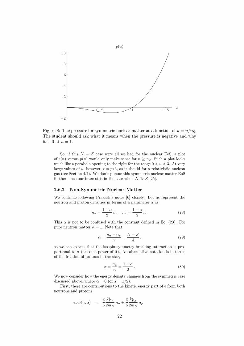
Given ε(n) from Eq. (69) one can find the pressure using Eq. (13),

p(n) = n2 d

dn

( ε

n

)

= n0

[

2

3

⟨

E0F

⟩

u5/3 +A

2u2 +

Bσ

σ + 1uσ+1

]

. (77)

For the parameters of Eq. (76) its dependence on n is shown in Fig. 8. Onfirst seeing this graph, the student should wonder why p(u = 1) = p(n0) =0. And, what is the meaning of the negative values for pressure belowu = 1? (Hint: what is “cavitation”?)

21

p(u)

0.5 1 1.5u

-2

2

4

6

8

10

Figure 8: The pressure for symmetric nuclear matter as a function of u = n/n0.The student should ask what it means when the pressure is negative and whyit is 0 at u = 1.

So, if this N = Z case were all we had for the nuclear EoS, a plotof ε(n) versus p(n) would only make sense for n ≥ n0. Such a plot looksmuch like a parabola opening to the right for the range 0 < u < 3. At verylarge values of u, however, ε ≈ p/3, as it should for a relativistic nucleongas (see Section 4.2). We don’t pursue this symmetric nuclear matter EoSfurther since our interest is in the case when N � Z [25].

2.6.2 Non-Symmetric Nuclear Matter

We continue following Prakash’s notes [6] closely. Let us represent theneutron and proton densities in terms of a parameter α as

nn =1 + α

2n , np =

1 − α

2n . (78)

This α is not to be confused with the constant defined in Eq. (23). Forpure neutron matter α = 1. Note that

α =nn − np

n=

N − Z

A, (79)

so we can expect that the isospin-symmetry-breaking interaction is pro-portional to α (or some power of it). An alternative notation is in termsof the fraction of protons in the star,

x =np

n=

1 − α

2. (80)

We now consider how the energy density changes from the symmetric casediscussed above, where α = 0 (or x = 1/2).

First, there are contributions to the kinetic energy part of ε from bothneutrons and protons,

εKE(n, α) =3

5

k2F,n

2mNnn +

3

5

k2F,p

2mNnp

22

= n 〈EF 〉1

2

[

(1 + α)5/3

+ (1 − α)5/3

]

, (81)

where

〈EF 〉 =3

5

h2

2mN

(

3π2n

2

)2/3

(82)

is the mean kinetic energy of symmetric nuclear matter at density n. Forn = n0 we note that 〈EF 〉 = 3

⟨

E0F

⟩

/5 [see Eq. (69)]. For non-symmetricmatter, α 6= 0, the excess kinetic energy is

∆εKE(n, α) = εKE(n, α) − εKE(n, 0)

= n 〈EF 〉{

1

2

[

(1 + α)5/3

+ (1 − α)5/3

]

− 1

}

= n 〈EF 〉{

22/3[

(1 − x)5/3 + x5/3]

− 1}

. (83)

For pure neutron matter, α = 1,

∆εKE(n, α) = n 〈EF 〉(

22/3 − 1)

. (84)

It is also useful to expand to leading order in α,

∆εKE(n, α) = n 〈EF 〉5

9α2

(

1 +α2

27+ · · ·

)

(85)

= n EFα2

3

(

1 +α2

27+ · · ·

)

. (86)

Keeping terms to order α2 is evidently good enough for most purposes.For pure neutron matter, the energy per particle (which, recall, is ε/n) atnormal density is ∆εKE(n0, 1)/n0 ≈ 13 MeV, more than a third of thetotal bulk symmetry energy of 30 MeV, our fourth nuclear parameter.

Thus the potential energy contribution to the bulk symmetry energymust be 20 MeV or so. Let us assume the quadratic approximation in αalso works well enough for this potential contribution and write the totalenergy per particle as

E(n, α) = E(n, 0) + α2S(n) , (87)

The isospin-symmetry breaking is proportional to α2, which reflects (roughly)the pair-wise nature of the nuclear interactions.

We will assume S(u), u = n/n0, has the form

S(u) = (22/3 − 1)3

5

⟨

E0F

⟩

(

u2/3 − F (u))

+ S0F (u) . (88)

Here S0 = 30 MeV is the bulk symmetry energy parameter. The functionF (u) must satisfy F (1) = 1 [so that S(u = 1) = S0] and F (0) = 0 [so thatS(u = 0) = 0; no matter means no energy]. Besides these two constraintsthere is, from what we presently know, a lot of freedom in what one choosesfor F (u). We will make the simplest possible choice here, namely,

F (u) = u , (89)

but we encourage the student to try other forms satisfying the conditionson F (u), such as

√u, to see what difference it makes.

23

E(n, α = 1) − mN

0.5 1 1.5 2u

20

40

60

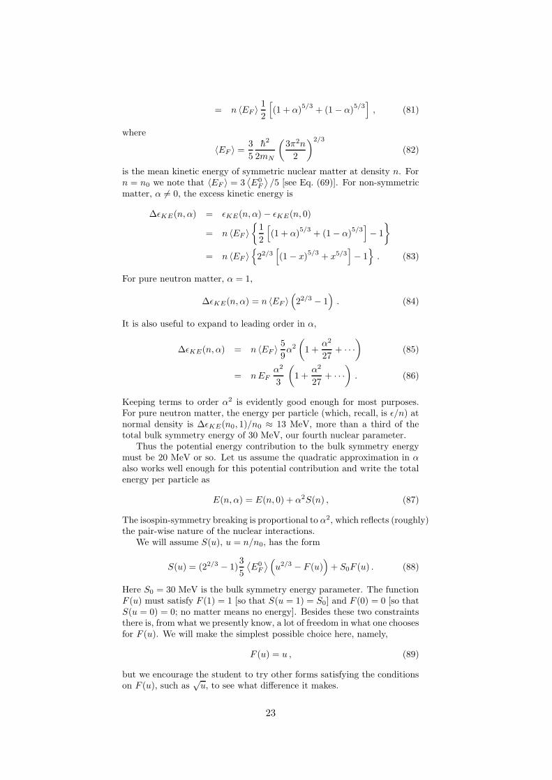
Figure 9: The average energy per neutron (less its rest mass), in MeV, for pureneutron matter, as a function of u = n/n0. The parameters for this curve arefor a nuclear compressibility K0 of 400 MeV.

Figure 9 shows the energy per particle for pure neutron matter, E(n, 1)−mN , as a function of u for the parameters of Eq. (76) and S0 = 30 MeV.In contrast with the α = 0 plot in Fig. 7, E(n, 1) ≥ 0 and is monotonicallyincreasing. The plot looks almost quadratic as a function of u. The domi-nant term at large u goes like uσ , and σ = 2.112 (for this case). However,one might have expected a linear increase instead. We will return to thispoint in Sec. 6.3.

Given the energy density, ε(n, α) = n0uE(n, α), the correspondingpressure is, from Eq. (13),

p(n, x) = ud

duε(n, α) − ε(n, α)

= p(n, 0) + n0α2

[

22/3 − 1

5

⟨

E0F

⟩

(

2u5/3 − 3u2)

+ S0u2

]

,(90)

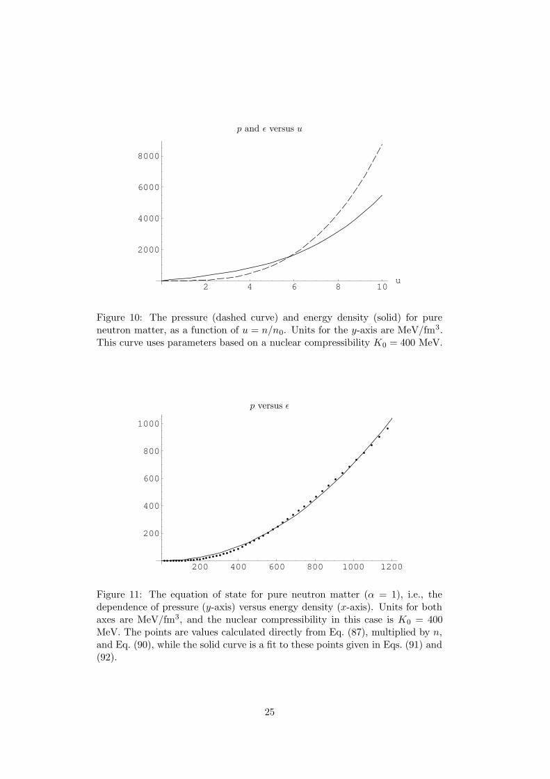
where p(n, 0) is defined by Eq. (77). Figure 10 shows the dependenceof the pure neutron p(n, 1) and ε(n, 1) on u = n/n0, ranging from 0 to10 times normal nuclear density. Both functions increase smoothly andmonotonically from u = 0. We hope the student would wonder why thepressure becomes greater than the energy density around u = 6. Whydoesn’t it go like a relativistic nucleon gas, p = ε/3? (Hint: check theassumptions.)

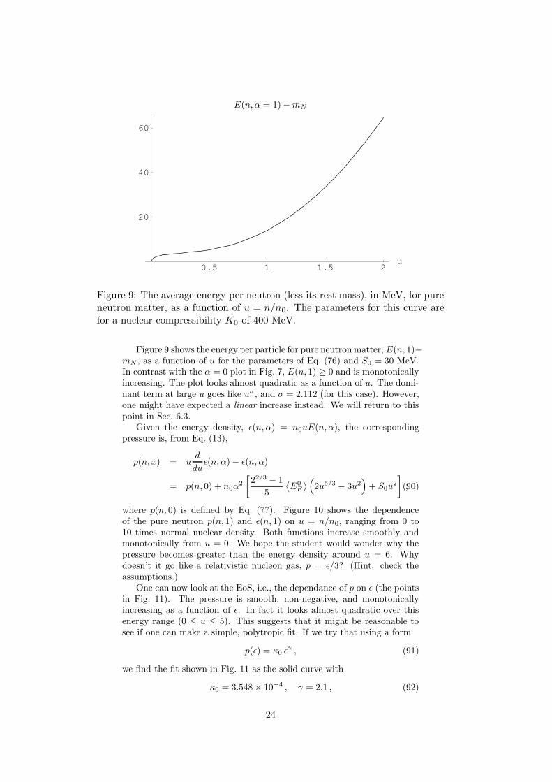
One can now look at the EoS, i.e., the dependance of p on ε (the pointsin Fig. 11). The pressure is smooth, non-negative, and monotonicallyincreasing as a function of ε. In fact it looks almost quadratic over thisenergy range (0 ≤ u ≤ 5). This suggests that it might be reasonable tosee if one can make a simple, polytropic fit. If we try that using a form

p(ε) = κ0 εγ , (91)

we find the fit shown in Fig. 11 as the solid curve with

κ0 = 3.548× 10−4 , γ = 2.1 , (92)

24

p and ε versus u

2 4 6 8 10u

2000

4000

6000

8000

Figure 10: The pressure (dashed curve) and energy density (solid) for pureneutron matter, as a function of u = n/n0. Units for the y-axis are MeV/fm3.This curve uses parameters based on a nuclear compressibility K0 = 400 MeV.

p versus ε

200 400 600 800 1000 1200

200

400

600

800

1000

Figure 11: The equation of state for pure neutron matter (α = 1), i.e., thedependence of pressure (y-axis) versus energy density (x-axis). Units for bothaxes are MeV/fm3, and the nuclear compressibility in this case is K0 = 400MeV. The points are values calculated directly from Eq. (87), multiplied by n,and Eq. (90), while the solid curve is a fit to these points given in Eqs. (91) and(92).

25

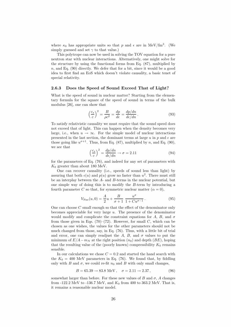
where κ0 has appropriate units so that p and ε are in MeV/fm3. (Wesimply guessed and set γ to that value.)

This polytrope can now be used in solving the TOV equation for a pureneutron star with nuclear interactions. Alternatively, one might solve forthe structure by using the functional forms from Eq. (87), multiplied byn, and Eq. (90) directly. We defer that for a bit, since it would be a goodidea to first find an EoS which doesn’t violate causality, a basic tenet ofspecial relativity.

2.6.3 Does the Speed of Sound Exceed That of Light?

What is the speed of sound in nuclear matter? Starting from the elemen-tary formula for the square of the speed of sound in terms of the bulkmodulus [26], one can show that

(cs

c

)2

=B

ρc2=

dp

dε=

dp/dn

dε/dn. (93)

To satisfy relativistic causality we must require that the sound speed doesnot exceed that of light. This can happen when the density becomes verylarge, i.e., when u → ∞. For the simple model of nuclear interactionspresented in the last section, the dominant terms at large u in p and ε arethose going like uσ+1. Thus, from Eq. (87), multiplied by n, and Eq. (90),we see that

(cs

c

)2

=dp/dn

dε/dn→ σ = 2.11 (94)

for the parameters of Eq. (76), and indeed for any set of parameters withK0 greater than about 180 MeV.

One can recover causality (i.e., speeds of sound less than light) byassuring that both ε(u) and p(u) grow no faster than u2. There must stillbe an interplay between the A- and B-terms in the nuclear potential, butone simple way of doing this is to modify the B-term by introducing afourth parameter C so that, for symmetric nuclear matter (α = 0),

VNuc(u, 0) =A

2u +

B

σ + 1

uσ

1 + Cuσ−1. (95)

One can choose C small enough so that the effect of the denominator onlybecomes appreciable for very large u. The presence of the denominatorwould modify and complicate the constraint equations for A, B, and σfrom those given in Eqs. (70)–(72). However, for small C, which can bechosen as one wishes, the values for the other parameters should not bemuch changed from those, say, in Eq. (76). Thus, with a little bit of trialand error, one can simply readjust the A, B, and σ values to put theminimum of E/A−mN at the right position (n0) and depth (BE), hopingthat the resulting value of the (poorly known) compressibility K0 remainssensible.

In our calculations we chose C = 0.2 and started the hand search withthe K0 = 400 MeV parameters in Eq. (76). We found that, by fiddlingonly with B and σ, we could re-fit n0 and B with only small changes,

B = 65.39 → 83.8 MeV , σ = 2.11 → 2.37 , (96)

somewhat larger than before. For these new values of B and σ, A changesfrom -122.2 MeV to -136.7 MeV, and K0 from 400 to 363.2 MeV. That is,it remains a reasonable nuclear model.

26

One can now proceed as in the last section to get ε(n, α), p(n, α), andthe EoS, p(ε, α). The results are not much different from those shown inthe figures of the previous sub-section. This time we decided to live witha quadratic fit for the EoS for pure neutron matter, finding

p(ε, 1) = κ0ε2 , κ0 = 4.012× 10−4 . (97)

This is not much different from before, Eq. (92). Somewhat more usefulfor solving the TOV equation is to express ε in terms of p,

ε(p) = (p/κ0))1/2

. (98)

2.6.4 Pure Neutron Star with Nuclear Interactions

Having laid all this groundwork, the student can now proceed to solve theTOV equations as before for a pure neutron star, using the fit for ε(p)found in the previous sub-section. It is, once again, useful to convert fromthe units of MeV/fm3 to ergs/cm3 to M�/km3 and dimensionless p andε. By now the student has undoubtedly grown quite accustomed to thatprocedure.

ε(p) = (κ0ε0)−1/2p1/2 = A0p

1/2 , A0 = 0.8642 , (99)

where this time we defined

ε0 =m4

nc5

3π2h3 . (100)

With this, the constant α that occurs on the right-hand side of the TOVequation, Eq. (22), is α = A0R0 = 1.276 km. The constant for the massequation, Eq. (25), is β = 0.03265, again in units of 1/km3.

Now proceeding as before, one can solve the coupled TOV equationsfor p(r) and M(r) for various initial central pressures, p(0). We don’texhibit here plots of the solutions, as they look very similar to those forthe Fermi gas EoS, Fig. 5.

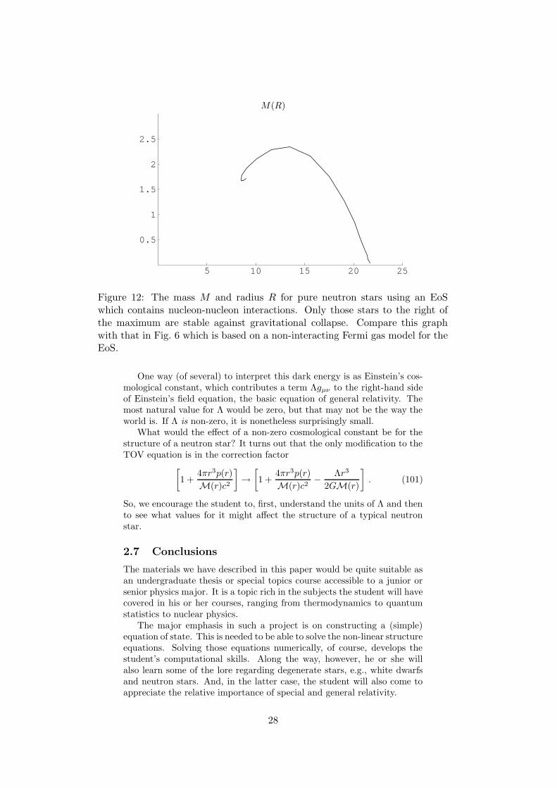
More interesting is to solve for a range of initial p(0)’s, generating, asbefore, a mass M versus radius R plot which now includes nucleon-nucleoninteractions (Fig. 12). The effect of the nuclear potential is enormous, oncomparing with the Fermi gas model predictions for M vs. R shown inFig. 6. The maximum star mass this time is about 2.3 M�, rather than 0.8M�. The radius for this maximum mass star is about 13.5 km, somewhatlarger than the Fermi gas model radius of 11 km. The large value ofmaximum M is a reflection of the large value of nuclear (in)compressibilityK0 = 363 MeV. The more incompressible something is, the more mass itcan support. Had we fit to a smaller value of K0 we would have gotten asmaller maximum mass.

2.6.5 What About a Cosmological Constant?

We do not know (either) if there is one, but there are definite indica-tions that a great part of the make-up of our universe is something called“Dark Energy” [27]. This conclusion comes about because we have re-cently learned that something, at the present time, is causing the universeto be accelerating, instead of slowing down (as would be expected afterthe Big Bang).

27

M(R)

5 10 15 20 25

0.5

1

1.5

2

2.5

Figure 12: The mass M and radius R for pure neutron stars using an EoSwhich contains nucleon-nucleon interactions. Only those stars to the right ofthe maximum are stable against gravitational collapse. Compare this graphwith that in Fig. 6 which is based on a non-interacting Fermi gas model for theEoS.

One way (of several) to interpret this dark energy is as Einstein’s cos-mological constant, which contributes a term Λgµν to the right-hand sideof Einstein’s field equation, the basic equation of general relativity. Themost natural value for Λ would be zero, but that may not be the way theworld is. If Λ is non-zero, it is nonetheless surprisingly small.

What would the effect of a non-zero cosmological constant be for thestructure of a neutron star? It turns out that the only modification to theTOV equation is in the correction factor

[

1 +4πr3p(r)

M(r)c2

]

→[

1 +4πr3p(r)

M(r)c2− Λr3

2GM(r)

]

. (101)

So, we encourage the student to, first, understand the units of Λ and thento see what values for it might affect the structure of a typical neutronstar.

2.7 Conclusions

The materials we have described in this paper would be quite suitable asan undergraduate thesis or special topics course accessible to a junior orsenior physics major. It is a topic rich in the subjects the student will havecovered in his or her courses, ranging from thermodynamics to quantumstatistics to nuclear physics.

The major emphasis in such a project is on constructing a (simple)equation of state. This is needed to be able to solve the non-linear structureequations. Solving those equations numerically, of course, develops thestudent’s computational skills. Along the way, however, he or she willalso learn some of the lore regarding degenerate stars, e.g., white dwarfsand neutron stars. And, in the latter case, the student will also come toappreciate the relative importance of special and general relativity.

28

References

[1] It is widely beleived that neutron stars were proposed by Lev Landauin 1932, very soon after the neutron was discovered (although we arenot aware of any documented proof of this). In 1934 Fritz Zwickyand Walter Baade speculated that they might be formed in Type IIsupernova explosions, which is now generally accepted as true.

[2] An on-line catalog of pulsars can be found athttp:/pulsar.princeton.edu.

[3] An intermediate-level on-line tutorial on the physics of pulsars can befound at http://www.jb.man.ac.uk/research/pulsar. This tutorial fol-lows the book by Andrew G. Lyne and Francis Graham-Smith, Pulsar

Astronomy, 2nd. ed., Cambridge University Press, 1998.

[4] R. C. Tolman, Phys. Rev. 55, 364 (1939); J. R. Oppenheimer and G.M. Volkov, Phys. Rev. 55, 374 (1939).

[5] Steven Weinberg, Gravitation and Cosmology, John Wiley & Sons,Inc., New York, 1972, Chapter 11.

[6] M. Prakash, lectures delivered at the Winter School on “The Equationof State of Nuclear Matter,” Puri, India, January 1994, esp. Chapter 3,Equation of State. These notes are published in “The Nuclear Equationof State”, ed. by A. Ausari and L. Satpathy, World Scientific PublishingCo., Singapore, 1996.

[7] R. Balian and J.-P. Blaizot, “Stars and Statistical Physics: A TeachingExperience,” Am. J. Phys. 67, (12) 1189 (1999).

[8] S. L. Shapiro and S. A. Teukolsky, Black Holes, White Dwarfs and

Neutron Stars: The Physics of Compact Objects, Wiley-Interscience,1983.

[9] We apologize to readers who are enthusiasts of SI units, but the firstauthor was raised on CGS units. Actually, we strongly feel that by thetime a physics student is at this level, he or she ought to be comfortablein switching from one system of units to another.

[10] A discussion of how to solve these equations (using conventional pro-gramming languages) is given in S. Koonin, Computational Physics,Benjamin-Cummings Publishing, 1986.

[11] For more details on white dwarfs, NASA provides a useful web pageat http://imagine.gsfc.nasa.gov/docs/science/know l1/dwarfs.html.

[12] This maximum mass of 1.4 M� is usually referred to as the Chan-drasekhar limit. See S. Chandrasekhar’s 1983 Nobel Prize lecture,http://www.nobel.se/physics/laureates/1983/. For more detail see histreatise, An Introduction to the Study of Stellar Structure, Dover Pub-lications, New York, 1939.

[13] Mathematica is a software product of Wolfram Research, Inc., (seeweb page at http://www.wolfram.com), and its use is described by S.Wolfram in The Mathematica Book, Fourth Ed., Cambridge Univer-sity Press, Cambridge, England, 1999. However, whenever we use thephrase “using Mathematica,” we really mean using whatever pack-age one has available or is familiar with, be it Maple, MathCad, orwhatever. We did almost all of the numerical/symbolic work that wedescribe in this paper in Mathematica, but some of its notebooks wereduplicated in MathCad, just to be sure it could be done there as well.

29

[14] Enough of these explicit flags! Most of the equations from here onpresent challenges for the student to work through.

[15] For the Newtonian case, a polytropic EoS also allows for a some-what more analytic solution in terms of Lane-Emden functions. SeeWeinberg, op. cit., Sec. 11.3, or C. Flynn, Lectures on Stellar Physics,especially lectures 4 and 5, at http://www.astro.utu.fi/ cflynn/Stars/.

[16] Despite the appearance of the 4πε0, the astute student will not belulled into thinking that this factor has anything to do with a Coulombpotential or the dielectric constant of the vacuum.

[17] Note that the right-hand side of Eq. (22) is negative (for positive p),so p(r) must fall monotonically from p(0).

[18] We leave this for the student to figure out, except for the followinghint: Use an if statement if necessary.

[19] This fit is least accurate (≈ 2%) at very low values of kF . However,this is where the pure neutron approximation itself is least accurate.The surface of a neutron star is likely made of elements like iron. Afictional account of what life might be like on such a surface can befound in Robert Forward’s Dragon’s Egg, first published in 1981 by DelRey Publishing, republished in 2000.

[20] See Weinberg, op. cit., Sec. 11.2.

[21] Because it is almost non-interacting with nuclear matter, a neutrinotends to escape from the neutron star. This is the major cooling mech-anism as the neutron star is being formed in a supernova explosion.George Gamow named this the URCA process, after a Brazilian casinowhere people lost a lot of money.

[22] Does the student know how to put all the factors of c back into ε0 soas to re-write this for CGS units?

[23] See, e.g., J. M. Blatt and V. F. Weisskopf, Theoretical Nuclear

Physics, John Wiley & Sons, 1952, Chap. 6, Sec. 2, or A. Bohr and B.R.Mottelson, Struktur der Atomkerne, Akademie-Verlag, Berlin 1975.

[24] The reason for the “(in)” is because a materials physicist might ratherdefine compressibility as χ = −(1/V )(∂V/∂p) = −(1/n)(dp/dn)−1.

[25] Folks interested in RHIC physics might want to, however. (RHICstands for “Relativistic Heavy Ion Collider,” an accelerator at theBrookhaven National Laboratory which is studying reactions like Aunuclei striking each other at center of mass energies around 200GeV/nucleon.)

[26] See, e.g., Hugh Young, University Physics, 8th ed., Addison-Wesley,Reading MA, 1992, Sec. 19-5, Speed of a Longitudinal Wave.

[27] See, e.g., P. J. E. Peebles and Bharat Ratra, Rev. Mod. Phys. 75,599 (2003)

[28] W. Y. Pauchy Hwang, private communication.

30