1

Synthesis of a Cyberphysical Hybrid MicrofluidicPlatform for Single-Cell Analysis

Mohamed Ibrahim, Student Member, IEEE, Krishnendu Chakrabarty, Fellow, IEEE,and Ulf Schlichtmann, Member, IEEE

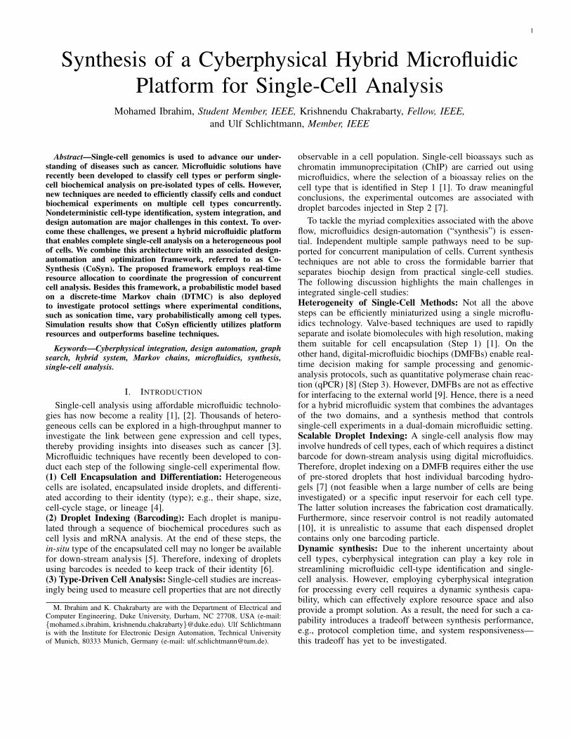
Abstract—Single-cell genomics is used to advance our under-standing of diseases such as cancer. Microfluidic solutions haverecently been developed to classify cell types or perform single-cell biochemical analysis on pre-isolated types of cells. However,new techniques are needed to efficiently classify cells and conductbiochemical experiments on multiple cell types concurrently.Nondeterministic cell-type identification, system integration, anddesign automation are major challenges in this context. To over-come these challenges, we present a hybrid microfluidic platformthat enables complete single-cell analysis on a heterogeneous poolof cells. We combine this architecture with an associated design-automation and optimization framework, referred to as Co-Synthesis (CoSyn). The proposed framework employs real-timeresource allocation to coordinate the progression of concurrentcell analysis. Besides this framework, a probabilistic model basedon a discrete-time Markov chain (DTMC) is also deployedto investigate protocol settings where experimental conditions,such as sonication time, vary probabilistically among cell types.Simulation results show that CoSyn efficiently utilizes platformresources and outperforms baseline techniques.

Keywords—Cyberphysical integration, design automation, graphsearch, hybrid system, Markov chains, microfluidics, synthesis,single-cell analysis.

I. INTRODUCTION

Single-cell analysis using affordable microfluidic technolo-gies has now become a reality [1], [2]. Thousands of hetero-geneous cells can be explored in a high-throughput manner toinvestigate the link between gene expression and cell types,thereby providing insights into diseases such as cancer [3].Microfluidic techniques have recently been developed to con-duct each step of the following single-cell experimental flow.(1) Cell Encapsulation and Differentiation: Heterogeneouscells are isolated, encapsulated inside droplets, and differenti-ated according to their identity (type); e.g., their shape, size,cell-cycle stage, or lineage [4].(2) Droplet Indexing (Barcoding): Each droplet is manipu-lated through a sequence of biochemical procedures such ascell lysis and mRNA analysis. At the end of these steps, thein-situ type of the encapsulated cell may no longer be availablefor down-stream analysis [5]. Therefore, indexing of dropletsusing barcodes is needed to keep track of their identity [6].(3) Type-Driven Cell Analysis: Single-cell studies are increas-ingly being used to measure cell properties that are not directly

M. Ibrahim and K. Chakrabarty are with the Department of Electrical andComputer Engineering, Duke University, Durham, NC 27708, USA (e-mail:{mohamed.s.ibrahim, krishnendu.chakrabarty}@duke.edu). Ulf Schlichtmannis with the Institute for Electronic Design Automation, Technical Universityof Munich, 80333 Munich, Germany (e-mail: ulf.schlichtmann@tum.de).

observable in a cell population. Single-cell bioassays such aschromatin immunoprecipitation (ChIP) are carried out usingmicrofluidics, where the selection of a bioassay relies on thecell type that is identified in Step 1 [1]. To draw meaningfulconclusions, the experimental outcomes are associated withdroplet barcodes injected in Step 2 [7].

To tackle the myriad complexities associated with the aboveflow, microfluidics design-automation (“synthesis”) is essen-tial. Independent multiple sample pathways need to be sup-ported for concurrent manipulation of cells. Current synthesistechniques are not able to cross the formidable barrier thatseparates biochip design from practical single-cell studies.The following discussion highlights the main challenges inintegrated single-cell studies:Heterogeneity of Single-Cell Methods: Not all the abovesteps can be efficiently miniaturized using a single microflu-idics technology. Valve-based techniques are used to rapidlyseparate and isolate biomolecules with high resolution, makingthem suitable for cell encapsulation (Step 1) [1]. On theother hand, digital-microfluidic biochips (DMFBs) enable real-time decision making for sample processing and genomic-analysis protocols, such as quantitative polymerase chain reac-tion (qPCR) [8] (Step 3). However, DMFBs are not as effectivefor interfacing to the external world [9]. Hence, there is a needfor a hybrid microfluidic system that combines the advantagesof the two domains, and a synthesis method that controlssingle-cell experiments in a dual-domain microfluidic setting.Scalable Droplet Indexing: A single-cell analysis flow mayinvolve hundreds of cell types, each of which requires a distinctbarcode for down-stream analysis using digital microfluidics.Therefore, droplet indexing on a DMFB requires either the useof pre-stored droplets that host individual barcoding hydro-gels [7] (not feasible when a large number of cells are beinginvestigated) or a specific input reservoir for each cell type.The latter solution increases the fabrication cost dramatically.Furthermore, since reservoir control is not readily automated[10], it is unrealistic to assume that each dispensed dropletcontains only one barcoding particle.Dynamic synthesis: Due to the inherent uncertainty aboutcell types, cyberphysical integration can play a key role instreamlining microfluidic cell-type identification and single-cell analysis. However, employing cyberphysical integrationfor processing every cell requires a dynamic synthesis capa-bility, which can effectively explore resource space and alsoprovide a prompt solution. As a result, the need for such a ca-pability introduces a tradeoff between synthesis performance,e.g., protocol completion time, and system responsiveness—this tradeoff has yet to be investigated.

2

Stochasticity of Protocol Conditions: Despite the effortsmade towards standardization of single-cell protocols, manyprotocol steps, such as the duration of sonication in ChIP, aredeemed to be cell-type-specific. For example, CD4+ white-blood cells require significantly longer sonication time com-pared to other red blood cells [11]. Failing to characterize thevariation in sonication time and other parameters among celltypes may lead to degradation in down-stream immunoprecip-itation and thus the overall ChIP performance [12]. Hence, itis important to take into consideration such stochasticity whendefining the protocol guidelines.

In this paper, we address the above challenges by introduc-ing the first hybrid microfluidic platform for integrated single-cell analysis. We present a synthesis method, referred to asCo-Synthesis (CoSyn), to control the dual-domain platform.We also develop a probabilistic model that employs a discrete-time Markov chain (DTMC) to capture protocol settings whereexperimental parameters vary among cell types. The maincontributions of this paper are as follows:• We present an architecture of a hybrid microfluidic

platform that integrates digital-microfluidic and flow-based domains (using valves) for large-scale single-cellanalysis.

• We describe CoSyn, which enables coordinated controlof the microfluidic components, and allows dual-domainsynthesis for concurrent sample pathways.

• We propose two schemes for valve-based routing (graph-theoretic and incremental methods), which enable dy-namic routing of concurrent samples within a reconfig-urable valve-based system.

• We construct a DTMC model, which utilizes probabilis-tic information related to protocol steps and experimentbudget to investigate the efficiency of probabilistic pro-tocol decisions.

• We evaluate system performance and reconfigurabilitywhile exploring various configurations of the valve-based system.

The rest of the paper is organized as follows. Section IIpresents an overview of related prior work and probabilisticformal methods that are relevant to this work. An overviewof the hybrid microfluidic platform and its use for single-cell analysis are presented in Section III. Next, we formalizethe single-cell analysis flow in Section IV and describe theproposed synthesis framework (CoSyn) in Section V. Subse-quently, details of the valve-based synthesizer are introducedSection VI, and probabilistic protocol modeling is presentedin Section VII. Our experimental evaluation is presented inSection VIII and conclusions are drawn in Section IX.

II. PRELIMINARIES

In this section, we review synthesis methods for microfluidicbiochips and relevant modeling techniques related to stochasticprocesses.A. Synthesis of Microfluidic Platforms

A DMFB manipulates picoliter droplets, and consists ofa two-dimensional array of electrodes and a set of on-chipresources [13]. Valve-based biochips, on the other hand, rely

on special-purpose components (e.g., microvalves and micro-pumps) to manipulate liquid flow [14].

Considerable research efforts have been devoted to the syn-thesis of biochemical applications for a specific microfluidictechnology, e.g., either digital-microfluidic systems or valve-based systems. Early synthesis methods for both technologiesfocused on scheduling, droplet routing, chip-level routing,and sharing of control pins (or pressure sources) [15]–[26].However, these methods are inadequate for single-cell analysissince they can only be applied to single biochemical assays.Moreover, real-time coordination between different single-cell microfluidic techniques is not possible using these earlymethods.

Cyberphysical synthesis techniques have enabled onlineerror recovery [27]–[31], volume precision [32], terminationof biochemical applications such as qPCR [33], and protocolsfor multiple samples [34], [35]. However, a key limitation ofthe above methods is that they fail to support heterogeneoussingle-cell analysis, and considerable manual effort is requiredto coordinate biochemical procedures.

Therefore, to close the gap between microfluidics and single-cell genomics, there is a need for a synthesis framework thatcan coordinate single-cell analysis techniques.B. Discrete-Time Markov Chains and Stochastic Systems

DTMCs constitute a formal method to model stochasticsystems, such as in biology [36], that exhibit a discretestate space [37]. DTMCs are similar to finite-state machines,but enriched with probabilistic transitions to model randomphenomena. A transition from state si to state sj is associatedwith a one-step transition probability that must depend onlyon the two states and not on the previous transitions—thisproperty is referred to as Markov property.

Formally, a DTMC D is specified as a tuple D =〈S, sinit,U ,J 〉, where: (i) S is a finite set of states (statespace) and sinit ∈ S is the initial state; (ii) U : S ×S → [0, 1]is a transition probability matrix such that

∑s′∈S U(s, s′) =

1 ∀s ∈ S; (iii) J : S → 2AP is a labeling function that assignseach state to a set of atomic propositions from a denumerableproposition set AP [37]. These labels can be utilized by aprobabilistic model-checking tool to express DTMC modelproperties with the help of temporal logic.

Properties of a DTMC model can be described using Proba-bilistic Computation Tree Logic (PCTL) [38]. PCTL formulaeare interpreted over the DTMC states. For instance, considera predicate φ that is always satisfied in state s (i.e., s |= φ),we can use the following PCTL formulae to describe path ornumerical queries:

1) Q1 := P≥0.95[♦φ], which inquires if the modeledsystem can eventually reach a state that satisfies φ witha probability that is greater than or equal to 0.95. Theoperator ♦ means “eventually”.

2) Q2 := Pmax=?[♦<10φ], which seeks the maximumprobability that the system will eventually reach a states satisfying φ in less than 10 steps.

The query Q1 is considered to be a reachability query,whereas Q2 is a numerical query. These queries and others canbe used to investigate the evolution of a stochastic system that

3

Optical detector HeaterMagnet

Fluorescence detectors

“Cell differentiation”

Interfacing electrode and

capacitive sensor (ec )

Capillary interface

Syringe pump source

+

Quantitative single-cell analysis

(e.g., DNA, RNA, epigenetics)

Isolated cellsCell

encapsulationBarcoding

droplet controlCell

Differentiation

Ring bus

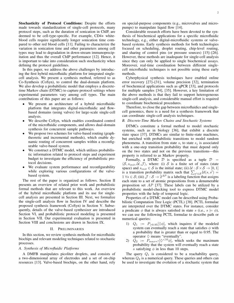
Fig. 1: The hybrid platform for single-cell analysis.

is modeled using DTMC. More details about DTMC modelchecking and PCTL syntax can be found in [38].

III. HYBRID PLATFORM AND SINGLE-CELL ANALYSIS

Single-cell analysis relies on the concurrent manipulationof sample droplets, where each sample cell is run throughthe protocol flow discussed in Section I. An efficient on-chip implementation of the single-cell analysis protocol isaccomplished using a hybrid platform. Fig. 1 shows theplatform components matched with different protocol stages.The two domains are connected through a capillary interface;this technique has been successfully adopted in practice [10].

A. Cell Encapsulation and Flow ControlAs shown in Fig. 1, on-chip operation starts with the

encapsulation of single cells in droplets, which is efficientlyaccomplished using flow-based microfluidics [10]. The dropletgenerator uses a syringe pump such that the flow rate ofpressure-driven droplets can be automatically controlled viafeedback. A capacitive sensor is placed at the interfacing elec-trode (ec in Fig. 1) on the digital side to sense a droplet [39].When the digital array is unable to accommodate additionaldroplets, it stops the flow by switching off the pump.

Note that an actuator is used in the flow-based component,whereas a sensor is placed on the digital side. To synchronizethe two domains, the flow-control procedure (capacitive sens-ing and pump control) is invoked at the same frequency asdroplet actuation in the digital domain (1 Hz to 10 Hz).

B. Cell DifferentiationAutomated cell-type identification can be achieved by ana-

lyzing signaling events in single cells in situ. Similar to theminiaturization of gene-expression analysis [40], a green fluo-rescent protein (GFP) reporter is used for cell differentiation.In each cell, the fluorescence intensity from the GFP (detectedin real-time using an on-chip fluorescence detector or imagingapparatus) is used to account for differences in expressionlevel among cells; this is equivalent to classifying cells intofunctional clusters that represent cell types.

Although a valve-based biochip can also be used for celldifferentiation, we consider a DMFB for this purpose due to its

3-electrode space

Two barcoding-droplet reservoirs

Four barcoding-droplet syringe pumps

Capilla

ry Valve-based microfluidic fabric—Crossbar

DMFB for mixing barcodes with samples

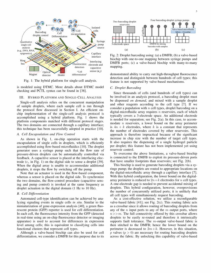
(a) (b) (c) Fig. 2: Droplet barcoding using: (a) a DMFB; (b) a valve-basedbiochip with one-to-one mapping between syringe pumps andDMFB ports; (c) a valve-based biochip with many-to-manymapping.

demonstrated ability to carry out high-throughput fluorescencedetection and distinguish between hundreds of cell types; thisfeature is not supported by valve-based mechanisms.

C. Droplet Barcoding

Since thousands of cells (and hundreds of cell types) canbe involved in an analysis protocol, a barcoding droplet mustbe dispensed on demand, and mixed with a sample dropletand other reagents according to the cell type [7]. If weconsider a population with n cell types, droplet barcoding on adigital-microfluidic array requires n reservoirs, each of whichtypically covers a 3-electrode space. An additional electrodeis needed for separation; see Fig. 2(a). In this case, to accom-modate n reservoirs, a lower bound on the array perimeteris 4n + k electrodes, where k is a constant that representsthe number of electrodes covered by other reservoirs. Thisapproach is therefore impractical because of the significantincrease in chip size with the number of target cell types.It also requires the dispensing of a single hydrogel particleper droplet; this feature has not been implemented yet usingreservoir control.

To overcome the above limitations, a valve-based biochipis connected to the DMFB to exploit its pressure-driven portsthat have smaller footprints than reservoirs; see Fig. 2(b).

This biochip is used to generate barcoding droplets via a sy-ringe pump; the droplets are routed to appropriate locations onthe digital-microfluidic array through a capillary interface [7].With this hybrid configuration, the lower bound on the digital-array perimeter is reduced to 2n+k electrodes for n cell types.A one-electrode gap is needed to prevent accidental mixing ofdroplets. This hybrid configuration, however, overprovisionsthe number of concurrently utilized ports; it is unlikely thatall cell types will simultaneously request barcoding.

As a cost-effective solution, we utilize a reconfigurablevalve-based fabric [41]; see Fig. 2(c). This routing fabric actsas a crossbar since it allows routing of barcoding droplets fromany of the n input ports to any of the m output ports, wheren>>m. The full connectivity offered by this crossbar allowsdroplets to be easily re-routed and therefore it intrinsicallysupports fault tolerance. The m-output valve-based fabric isthen stitched to the DMFB; hence the lower bound on theperimeter is decreased to 2m+k. However, in this situation,p valves (p > 0) are necessary for routing barcoding dropletsacross the fabric. By unlocking this capability of valve-based

4

(a) (b)

(c) (d)

Routing conflict 1st potential route2nd potential routeA routing channel

Valve

P1

P2

P1

P2

P3P4

P1, P2, P3, P4: Possible routes within a transposer

P3

P4

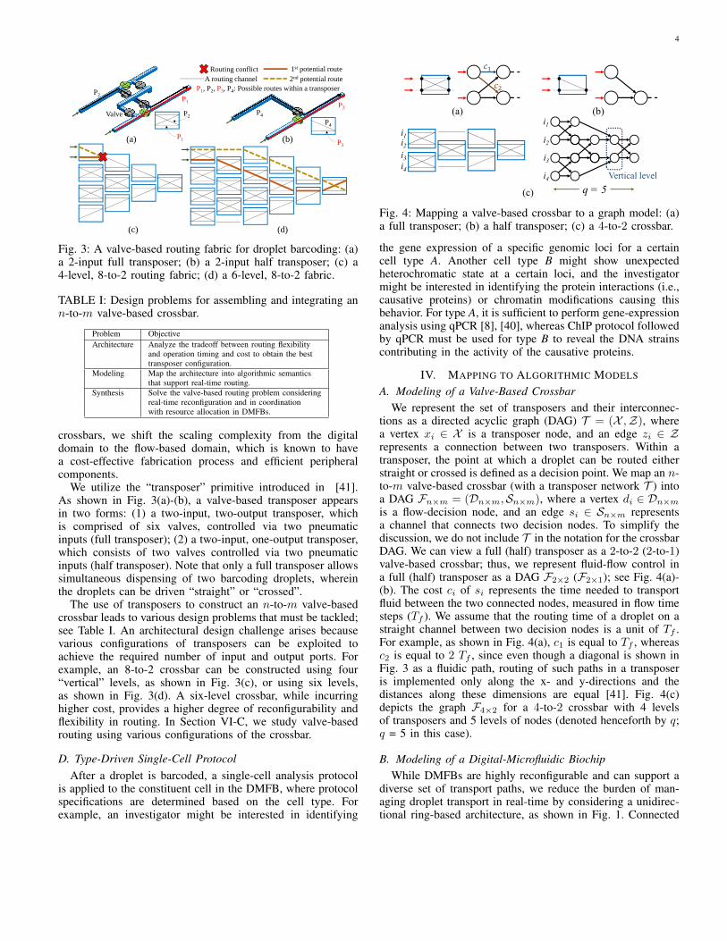
Fig. 3: A valve-based routing fabric for droplet barcoding: (a)a 2-input full transposer; (b) a 2-input half transposer; (c) a4-level, 8-to-2 routing fabric; (d) a 6-level, 8-to-2 fabric.

TABLE I: Design problems for assembling and integrating ann-to-m valve-based crossbar.

Problem ObjectiveArchitecture Analyze the tradeoff between routing flexibility

and operation timing and cost to obtain the besttransposer configuration.

Modeling Map the architecture into algorithmic semanticsthat support real-time routing.

Synthesis Solve the valve-based routing problem consideringreal-time reconfiguration and in coordinationwith resource allocation in DMFBs.

crossbars, we shift the scaling complexity from the digitaldomain to the flow-based domain, which is known to havea cost-effective fabrication process and efficient peripheralcomponents.

We utilize the “transposer” primitive introduced in [41].As shown in Fig. 3(a)-(b), a valve-based transposer appearsin two forms: (1) a two-input, two-output transposer, whichis comprised of six valves, controlled via two pneumaticinputs (full transposer); (2) a two-input, one-output transposer,which consists of two valves controlled via two pneumaticinputs (half transposer). Note that only a full transposer allowssimultaneous dispensing of two barcoding droplets, whereinthe droplets can be driven “straight” or “crossed”.

The use of transposers to construct an n-to-m valve-basedcrossbar leads to various design problems that must be tackled;see Table I. An architectural design challenge arises becausevarious configurations of transposers can be exploited toachieve the required number of input and output ports. Forexample, an 8-to-2 crossbar can be constructed using four“vertical” levels, as shown in Fig. 3(c), or using six levels,as shown in Fig. 3(d). A six-level crossbar, while incurringhigher cost, provides a higher degree of reconfigurability andflexibility in routing. In Section VI-C, we study valve-basedrouting using various configurations of the crossbar.

D. Type-Driven Single-Cell ProtocolAfter a droplet is barcoded, a single-cell analysis protocol

is applied to the constituent cell in the DMFB, where protocolspecifications are determined based on the cell type. Forexample, an investigator might be interested in identifying

(a) (b)

(c)

i1i2i3i4

ଵ

i1i2i3i4

ଶ

q = 5Vertical level

Fig. 4: Mapping a valve-based crossbar to a graph model: (a)a full transposer; (b) a half transposer; (c) a 4-to-2 crossbar.

the gene expression of a specific genomic loci for a certaincell type A. Another cell type B might show unexpectedheterochromatic state at a certain loci, and the investigatormight be interested in identifying the protein interactions (i.e.,causative proteins) or chromatin modifications causing thisbehavior. For type A, it is sufficient to perform gene-expressionanalysis using qPCR [8], [40], whereas ChIP protocol followedby qPCR must be used for type B to reveal the DNA strainscontributing in the activity of the causative proteins.

IV. MAPPING TO ALGORITHMIC MODELS

A. Modeling of a Valve-Based CrossbarWe represent the set of transposers and their interconnec-

tions as a directed acyclic graph (DAG) T = (X ,Z), wherea vertex xi ∈ X is a transposer node, and an edge zi ∈ Zrepresents a connection between two transposers. Within atransposer, the point at which a droplet can be routed eitherstraight or crossed is defined as a decision point. We map an n-to-m valve-based crossbar (with a transposer network T ) intoa DAG Fn×m = (Dn×m,Sn×m), where a vertex di ∈ Dn×mis a flow-decision node, and an edge si ∈ Sn×m representsa channel that connects two decision nodes. To simplify thediscussion, we do not include T in the notation for the crossbarDAG. We can view a full (half) transposer as a 2-to-2 (2-to-1)valve-based crossbar; thus, we represent fluid-flow control ina full (half) transposer as a DAG F2×2 (F2×1); see Fig. 4(a)-(b). The cost ci of si represents the time needed to transportfluid between the two connected nodes, measured in flow timesteps (Tf ). We assume that the routing time of a droplet on astraight channel between two decision nodes is a unit of Tf .For example, as shown in Fig. 4(a), c1 is equal to Tf , whereasc2 is equal to 2 Tf , since even though a diagonal is shown inFig. 3 as a fluidic path, routing of such paths in a transposeris implemented only along the x- and y-directions and thedistances along these dimensions are equal [41]. Fig. 4(c)depicts the graph F4×2 for a 4-to-2 crossbar with 4 levelsof transposers and 5 levels of nodes (denoted henceforth by q;q = 5 in this case).

B. Modeling of a Digital-Microfluidic BiochipWhile DMFBs are highly reconfigurable and can support a

diverse set of transport paths, we reduce the burden of man-aging droplet transport in real-time by considering a unidirec-tional ring-based architecture, as shown in Fig. 1. Connected

5

Barcode Propagation

Cell Identification

Active cell state: Barcoding Type-Driven Single-

Cell AnalysisCommit or

Discard

Identification & Labeling

Sample Dispense

Lysis bufferWater

Cell LysisBeads & primers

Elution buffer

mRNA Preparation

qPCR

Positive or Negative Control

+ve -ve

Report

Post-Fixation & Cell Lysis

DPBS & Glycine

CFG supernode CFG edge Dispense Mixing or dilution

Discard Detect Bead snapping Heat Sonicate

Chromatin Shearing

Beads & protein

antibody

Elution buffer

Immuno-precipitation and DNA washing (IPF)

qPCR

Positive or Negative Control

+ve -ve

Report

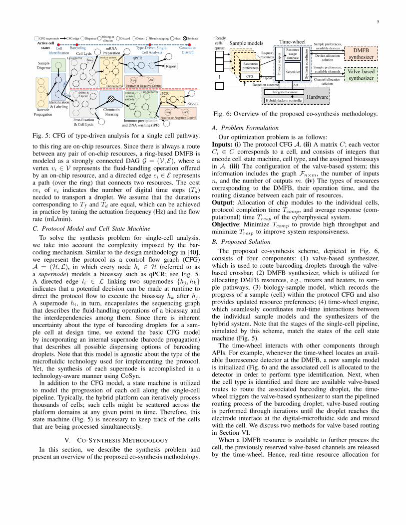
Fig. 5: CFG of type-driven analysis for a single cell pathway.

to this ring are on-chip resources. Since there is always a routebetween any pair of on-chip resources, a ring-based DMFB ismodeled as a strongly connected DAG G = (V, E), where avertex vi ∈ V represents the fluid-handling operation offeredby an on-chip resource, and a directed edge ei ∈ E representsa path (over the ring) that connects two resources. The costcei of ei indicates the number of digital time steps (Td)needed to transport a droplet. We assume that the durationscorresponding to Tf and Td are equal, which can be achievedin practice by tuning the actuation frequency (Hz) and the flowrate (mL/min).C. Protocol Model and Cell State Machine

To solve the synthesis problem for single-cell analysis,we take into account the complexity imposed by the bar-coding mechanism. Similar to the design methodology in [40],we represent the protocol as a control flow graph (CFG)A = (H,L), in which every node hi ∈ H (referred to asa supernode) models a bioassay such as qPCR; see Fig. 5.A directed edge li ∈ L linking two supernodes {hj , hk}indicates that a potential decision can be made at runtime todirect the protocol flow to execute the bioassay hk after hj .A supernode hi, in turn, encapsulates the sequencing graphthat describes the fluid-handling operations of a bioassay andthe interdependencies among them. Since there is inherentuncertainty about the type of barcoding droplets for a sam-ple cell at design time, we extend the basic CFG modelby incorporating an internal supernode (barcode propagation)that describes all possible dispensing options of barcodingdroplets. Note that this model is agnostic about the type of themicrofluidic technology used for implementing the protocol.Yet, the synthesis of each supernode is accomplished in atechnology-aware manner using CoSyn.

In addition to the CFG model, a state machine is utilizedto model the progression of each cell along the single-cellpipeline. Typically, the hybrid platform can iteratively processthousands of cells; such cells might be scattered across theplatform domains at any given point in time. Therefore, thisstate machine (Fig. 5) is necessary to keep track of the cellsthat are being processed simultaneously.

V. CO-SYNTHESIS METHODOLOGY

In this section, we describe the synthesis problem andpresent an overview of the proposed co-synthesis methodology.

Time-wheelDMFB

synthesizer

Valve-based synthesizer

Sample preferences, available channels

Channel-allocation solution

HardwareHybrid platform controller

Detection outcome

Resource usage

database

“Ready cells” queue

Sample models

Resources preferences

CFG Synt

hesi

s coo

rdin

ator

Update

Scheduler

Integrated sensors

Act

Prot

ocol

ada

pterRequest

resources

Sample preferences, available devices

Device-allocation solution

Fig. 6: Overview of the proposed co-synthesis methodology.

A. Problem FormulationOur optimization problem is as follows:

Inputs: (i) The protocol CFG A. (ii) A matrix C; each vectorCi ∈ C corresponds to a cell, and consists of integers thatencode cell state machine, cell type, and the assigned bioassaysin A. (iii) The configuration of the valve-based system; thisinformation includes the graph Fn×m, the number of inputsn, and the number of outputs m. (iv) The types of resourcescorresponding to the DMFB, their operation time, and therouting distance between each pair of resources.Output: Allocation of chip modules to the individual cells,protocol completion time Tcomp, and average response (com-putational) time Tresp of the cyberphysical system.Objective: Minimize Tcomp to provide high throughput andminimize Tresp to improve system responsiveness.

B. Proposed SolutionThe proposed co-synthesis scheme, depicted in Fig. 6,

consists of four components: (1) valve-based synthesizer,which is used to route barcoding droplets through the valve-based crossbar; (2) DMFB synthesizer, which is utilized forallocating DMFB resources, e.g., mixers and heaters, to sam-ple pathways; (3) biology-sample model, which records theprogress of a sample (cell) within the protocol CFG and alsoprovides updated resource preferences; (4) time-wheel engine,which seamlessly coordinates real-time interactions betweenthe individual sample models and the synthesizers of thehybrid system. Note that the stages of the single-cell pipeline,simulated by this scheme, match the states of the cell statemachine (Fig. 5).

The time-wheel interacts with other components throughAPIs. For example, whenever the time-wheel locates an avail-able fluorescence detector at the DMFB, a new sample modelis initialized (Fig. 6) and the associated cell is allocated to thedetector in order to perform type identification. Next, whenthe cell type is identified and there are available valve-basedroutes to route the associated barcoding droplet, the time-wheel triggers the valve-based synthesizer to start the pipelinedrouting process of the barcoding droplet; valve-based routingis performed through iterations until the droplet reaches theelectrode interface at the digital-microfluidic side and mixedwith the cell. We discuss two methods for valve-based routingin Section VI.

When a DMFB resource is available to further process thecell, the previously reserved valve-based channels are releasedby the time-wheel. Hence, real-time resource allocation for

6

Algorithm 1 DMFB Resource AllocationInput: Ci, G, current simulation time “t”Output: Assigned Resource “r”

1: R← GetCurrentlyUnoccupiedResources(G, t);2: if (R is empty) then return NULL;3: y ← GetOperationType(Ci);4: s← CalculateMinimumCostAllAvailableResources(y, R);5: if (s =∞) then return NULL; // No suitable resource6: r ← GetSelectedResource(s); return r;

the DMFB is also initiated by the time-wheel, which in turn,commits a cell pathway whenever its particular single-cellbioassays have executed. Based on an intermediate decisionpoint whose outcome is communicated to the sample model,the cell might also be discarded during analysis.C. DMFB Synthesizer

We use a greedy method to solve the resource-allocationproblem in the DMFB; the pseduocode is shown in Algo-rithm 1. We denote a DMFB resource by r ∈ Rd, where Rdencapsulates all DMFB resources. Thus, the cost of allocatingresource r to execute a fluidic operation of type y ∈ Y(the set Y incorporates all operation types) is ρ(r, r, y) =γ(r, y) + E(r, r), where γ(r, y) is the operation time on r andE(r, r) is the routing distance from r (the currently occupiedresource) to r. The worst-case computational complexity ofthis algorithm is O(|V|).

VI. VALVE-BASED SYNTHESIZER

Our goal is to design a fully connected fabric such that adroplet can be forwarded from any of the n inputs to anyof the m output ports. We present a sufficient criterion forachieving a fully connected fabric. The proof can be found inAppendix A.

Theorem 1. An n-to-m, q-level valve-based crossbar is a fullyconnected fabric if n and m are even integers, and q ≥ m+n

2 .

Using this theorem, we can automatically generate thegraph model Fn×m, thereby guaranteeing that any barcodinginput can reach all m outputs. The algorithm is described inAppendix B.

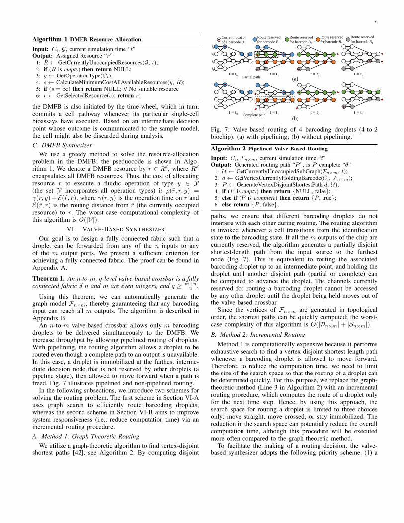
An n-to-m valve-based crossbar allows only m barcodingdroplets to be delivered simultaneously to the DMFB. Weincrease throughput by allowing pipelined routing of droplets.With pipelining, the routing algorithm allows a droplet to berouted even though a complete path to an output is unavailable.In this case, a droplet is immobilized at the furthest interme-diate decision node that is not reserved by other droplets (apipeline stage), then allowed to move forward when a path isfreed. Fig. 7 illustrates pipelined and non-pipelined routing.

In the following subsections, we introduce two schemes forsolving the routing problem. The first scheme in Section VI-Auses graph search to efficiently route barcoding droplets,whereas the second scheme in Section VI-B aims to improvesystem responsiveness (i.e., reduce computation time) via anincremental routing procedure.A. Method 1: Graph-Theoretic Routing

We utilize a graph-theoretic algorithm to find vertex-disjointshortest paths [42]; see Algorithm 2. By computing disjoint

i1

i2

i3

i4

Route reserved for barcode B1

Current location of a barcode Bi

Route reserved for barcode B2

Route reserved for barcode B3

Route reserved for barcode B4

(a)t = t0 t = t1 t = t2 t = t3

(b)t = t0 t = t1 t = t2 t = t3

Partial path

Complete path

Fig. 7: Valve-based routing of 4 barcoding droplets (4-to-2biochip): (a) with pipelining; (b) without pipelining.

Algorithm 2 Pipelined Valve-Based RoutingInput: Ci, Fn×m, current simulation time “t”Output: Generated routing path “P ”, is P complete “θ”

1: U ← GetCurrentlyUnoccupiedSubGraph(Fn×m, t);2: d← GetVertexCurrentlyHoldingBarcode(Ci, Fn×m);3: P ← GenerateVertexDisjointShortestPath(d, U);4: if (P is empty) then return {NULL, false};5: else if (P is complete) then return {P , true};6: else return {P , false};

paths, we ensure that different barcoding droplets do notinterfere with each other during routing. The routing algorithmis invoked whenever a cell transitions from the identificationstate to the barcoding state. If all the m outputs of the chip arecurrently reserved, the algorithm generates a partially disjointshortest-length path from the input source to the furthestnode (Fig. 7). This is equivalent to routing the associatedbarcoding droplet up to an intermediate point, and holding thedroplet until another disjoint path (partial or complete) canbe computed to advance the droplet. The channels currentlyreserved for routing a barcoding droplet cannot be accessedby any other droplet until the droplet being held moves out ofthe valve-based crossbar.

Since the vertices of Fn×m are generated in topologicalorder, the shortest paths can be quickly computed; the worst-case complexity of this algorithm is O(|Dn×m|+ |Sn×m|).

B. Method 2: Incremental RoutingMethod 1 is computationally expensive because it performs

exhaustive search to find a vertex-disjoint shortest-length pathwhenever a barcoding droplet is allowed to move forward.Therefore, to reduce the computation time, we need to limitthe size of the search space so that the routing of a droplet canbe determined quickly. For this purpose, we replace the graph-theoretic method (Line 3 in Algorithm 2) with an incrementalrouting procedure, which computes the route of a droplet onlyfor the next time step. Hence, by using this approach, thesearch space for routing a droplet is limited to three choicesonly: move straight, move crossed, or stay immobilized. Thereduction in the search space can potentially reduce the overallcomputation time, although this procedure will be executedmore often compared to the graph-theoretic method.

To facilitate the making of a routing decision, the valve-based synthesizer adopts the following priority scheme: (1) a

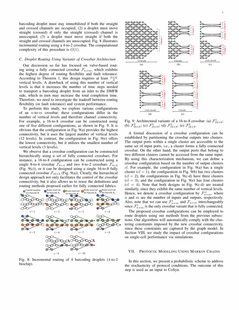
7

barcoding droplet must stay immobilized if both the straightand crossed channels are occupied; (2) a droplet must movestraight (crossed) if only the straight (crossed) channel isunoccupied; (3) a droplet must move straight if both thestraight and crossed channels are unoccupied. Fig. 8 illustratesincremental routing using a 4-to-2 crossbar. The computationalcomplexity of this procedure is O(1).

C. Droplet Routing Using Variants of Crossbar Architecture

Our discussion so far has focused on valve-based rout-ing using a fully connected crossbar Fn×m, which exhibitsthe highest degree of routing flexibility and fault tolerance.According to Theorem 1, this design requires at least n+m

2vertical levels. A drawback of using this number of verticallevels is that it increases the number of time steps neededto transport a barcoding droplet from an inlet to the DMFBside, which in turn may increase the total completion time.Therefore, we need to investigate the tradeoff between routingflexibility (or fault tolerance) and system performance.

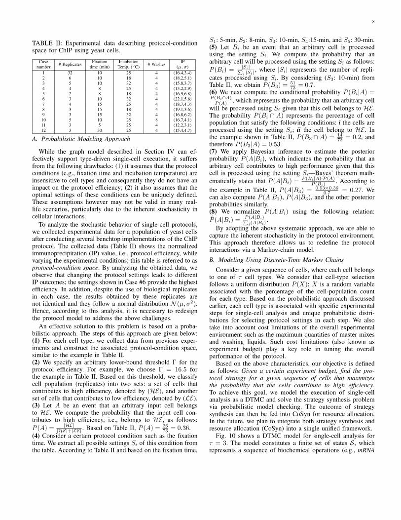
To perform this study, we explore various configurationsof an n-to-m crossbar; these configurations differ in thenumber of vertical levels and therefore channel connectivity.For example, a 16-to-8 crossbar can be constructed usingone of five different configurations, as shown in Fig. 9. It isobvious that the configuration in Fig. 9(a) provides the highestconnectivity, but it uses the largest number of vertical levels(12 levels). In contrast, the configuration in Fig. 9(e) offersthe lowest connectivity, but it utilizes the smallest number ofvertical levels (3 levels).

We observe that a crossbar configuration can be constructedhierarchically using a set of fully connected crossbars. Forinstance, a 16-to-8 configuration can be constructed using asingle 8-to-4 crossbar F8×4 and two 4-to-2 crossbars F4×2(Fig. 9(c)), or it can be designed using a single 16-to-8 fullyconnected crossbar F16×8 (Fig. 9(a)). Clearly, the hierarchicaldesign approach not only facilitates the control of the crossbarconnectivity, but it also allows us to reuse the definitions androuting methods proposed earlier for fully connected fabrics.

i1

i2

i3

i4

Route reserved for barcode B1

Current location of a barcode Bi

Route reserved for barcode B2

Route reserved for barcode B3

Route reserved for barcode B4

t = 1 t = 2 t = 3 t = 4

t = 5 t = 6 t = 7 t = 8

t = 9 t = 10

Fig. 8: Incremental routing of 4 barcoding droplets (4-to-2biochip).

12 levels(a)

6 levels(b)

Clu

ster

1

{3,6} levels

(c)

Clu

ster

2C

lust

er 1

{3,6} levels

(d)

Clu

ster

2C

lust

er 3

3 levels

(e)

Clu

ster

3C

lust

er 4

Clu

ster

1C

lust

er 2

Clu

ster

1C

lust

er 2

Clu

ster

3

Clu

ster

1

Fig. 9: Architectural variants of a 16-to-8 crossbar: (a) F116×8;

(b) F216×8; (c) F3

16×8; (d) F316×8; (e) F4

16×8.

A formal discussion of a crossbar configuration can beestablished by partitioning the crossbar outputs into clusters.The output ports within a single cluster are accessible to thesame set of input ports, i.e., a cluster forms a fully connectedcrossbar. On the other hand, the output ports that belong totwo different clusters cannot be accessed from the same input.By using this characterization mechanism, we can define acrossbar configuration based on the number of output clusterscl. For example, the configuration in Fig. 9(a) has a singlecluster (cl = 1), the configuration in Fig. 9(b) has two clusters(cl = 2), the configurations in Fig. 9(c-d) have three clusters(cl = 3), and the configuration in Fig. 9(e) has four clusters(cl = 4). Note that both designs in Fig. 9(c-d) are treatedsimilarly, since they exhibit the same number of vertical levels.Hence, we denote a crossbar configuration by Fcln×m, wheren and m are the number of inputs and outputs, respectively.Also, note that we can use F1

n×m and Fn×m interchangeablysince F1

n×m is the only crossbar variant that is fully connected.The proposed crossbar configurations can be employed to

route droplets using our methods from the previous subsec-tions. Our algorithms will automatically comply with the clus-tering constraints imposed by the new crossbar connectivity,since these constraints are captured by the graph model. InSection VIII, we study the impact of crossbar configurationson single-cell performance via simulations.

VII. PROTOCOL MODELING USING MARKOV CHAINS

In this section, we present a probabilistic scheme to addressthe stochasticity of protocol conditions. The outcome of thisstep is used as an input to CoSyn.

8

TABLE II: Experimental data describing protocol-conditionspace for ChIP using yeast cells.

Case # Replicates Fixation Incubation # Washes IPnumber time (min) Temp. (◦C) (µ, σ)

1 32 10 25 4 (16.4,3.4)2 6 10 18 4 (18.2,5.1)3 5 10 32 4 (15.8,3.7)4 4 8 25 4 (13.2,2.9)5 2 8 18 4 (16.9,6.8)6 3 10 32 4 (22.1,5.6)7 4 15 25 4 (18.7,4.3)8 3 15 18 4 (19.1,3.6)9 3 15 32 4 (16.8,6.2)10 5 10 25 8 (16.7,4.1)11 3 5 25 4 (12.2,3.1)12 3 30 25 4 (15.4,4.7)

A. Probabilistic Modeling Approach

While the graph model described in Section IV can ef-fectively support type-driven single-cell execution, it suffersfrom the following drawbacks: (1) it assumes that the protocolconditions (e.g., fixation time and incubation temperature) areinsensitive to cell types and consequently they do not have animpact on the protocol efficiency; (2) it also assumes that theoptimal settings of these conditions can be uniquely defined.These assumptions however may not be valid in many real-life scenarios, particularly due to the inherent stochasticity incellular interactions.

To analyze the stochastic behavior of single-cell protocols,we collected experimental data for a population of yeast cellsafter conducting several benchtop implementations of the ChIPprotocol. The collected data (Table II) shows the normalizedimmunoprecipitation (IP) value, i.e., protocol efficiency, whilevarying the experimental conditions; this table is referred to asprotocol-condition space. By analyzing the obtained data, weobserve that changing the protocol settings leads to differentIP outcomes; the settings shown in Case #6 provide the highestefficiency. In addition, despite the use of biological replicatesin each case, the results obtained by these replicates arenot identical and they follow a normal distribution N (µ, σ2).Hence, according to this analysis, it is necessary to redesignthe protocol model to address the above challenges.

An effective solution to this problem is based on a proba-bilistic approach. The steps of this approach are given below:(1) For each cell type, we collect data from previous exper-iments and construct the associated protocol-condition space,similar to the example in Table II.(2) We specify an arbitrary lower-bound threshold Γ for theprotocol efficiency. For example, we choose Γ = 16.5 forthe example in Table II. Based on this threshold, we classifycell population (replicates) into two sets: a set of cells thatcontributes to high efficiency, denoted by (HE), and anotherset of cells that contributes to low efficiency, denoted by (LE).(3) Let A be an event that an arbitrary input cell belongsto HE . We compute the probability that the input cell con-tributes to high efficiency, i.e., belongs to HE , as follows:P (A) = |HE|

|HE|+|LE| . Based on Table II, P (A) = 2673 = 0.36.

(4) Consider a certain protocol condition such as the fixationtime. We extract all possible settings Si of this condition fromthe table. According to Table II and based on the fixation time,

S1: 5-min, S2: 8-min, S3: 10-min, S4:15-min, and S5: 30-min.(5) Let Bi be an event that an arbitrary cell is processedusing the setting Si. We compute the probability that anarbitrary cell will be processed using the setting Si as follows:P (Bi) = |Si|∑

i |Si| , where |Si| represents the number of repli-cates processed using Si. By considering (S3: 10-min) fromTable II, we obtain P (B3) = 51

73 = 0.7.(6) We next compute the conditional probability P (Bi|A) =P (Bi∩A)P (A) , which represents the probability that an arbitrary cell

will be processed using Si given that this cell belongs to HE .The probability P (Bi ∩ A) represents the percentage of cellpopulation that satisfy the following conditions: i the cells areprocessed using the setting Si; ii the cell belong to HE . Inthe example shown in Table II, P (B3 ∩ A) = 14

73 = 0.2, andtherefore P (B3|A) = 0.53.(7) We apply Bayesian inference to estimate the posteriorprobability P (A|Bi), which indicates the probability that anarbitrary cell contributes to high performance given that thiscell is processed using the setting Si—Bayes’ theorem math-ematically states that P (A|Bi) = P (Bi|A)·P (A)

P (Bi). According to

the example in Table II, P (A|B3) = 0.53×0.360.7 = 0.27. We

can also compute P (A|B1), P (A|B3), and the other posteriorprobabilities similarly.(8) We normalize P (A|Bi) using the following relation:P (A|Bi) = P (A|Bi)∑

i(A|Bi).

By adopting the above systematic approach, we are able tocapture the inherent stochasticity in the protocol environment.This approach therefore allows us to redefine the protocolinteractions via a Markov-chain model.

B. Modeling Using Discrete-Time Markov Chains

Consider a given sequence of cells, where each cell belongsto one of τ cell types. We consider that cell-type selectionfollows a uniform distribution P (X); X is a random variableassociated with the percentage of the cell-population countfor each type. Based on the probabilistic approach discussedearlier, each cell type is associated with specific experimentalsteps for single-cell analysis and unique probabilistic distri-butions for selecting protocol settings in each step. We alsotake into account cost limitations of the overall experimentalenvironment such as the maximum quantities of master mixesand washing liquids. Such cost limitations (also known asexperiment budget) play a key role in tuning the overallperformance of the protocol.

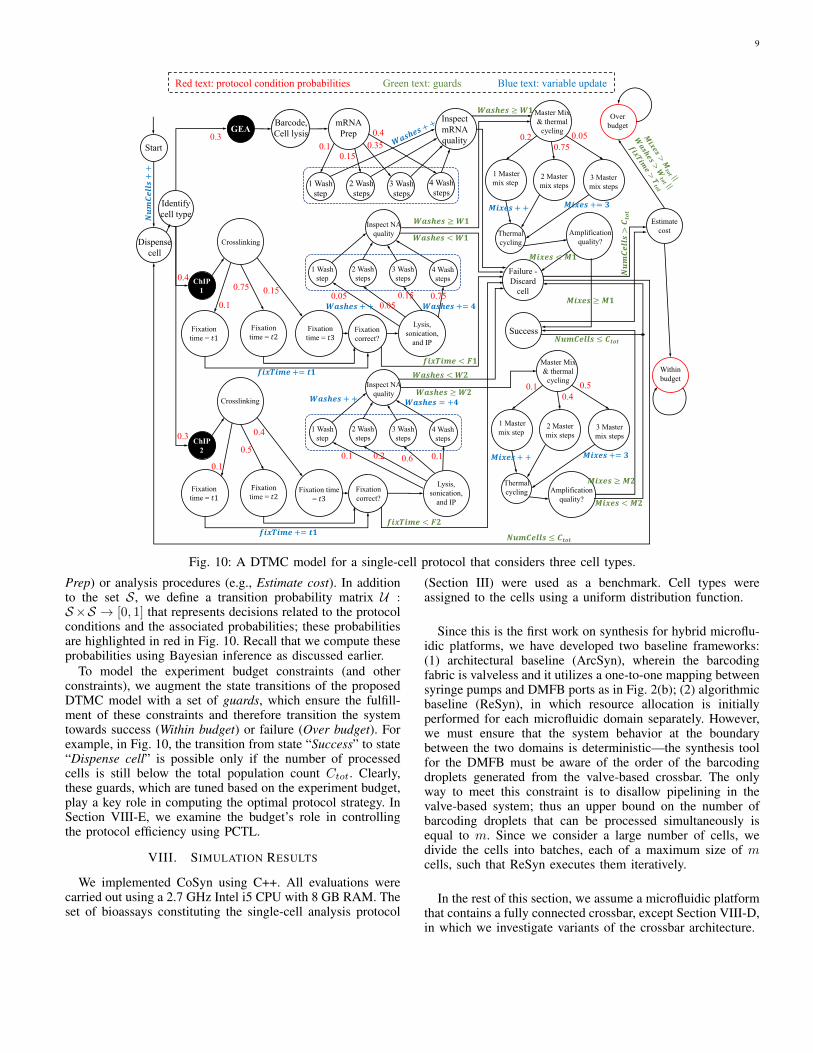
Based on the above characteristics, our objective is definedas follows: Given a certain experiment budget, find the pro-tocol strategy for a given sequence of cells that maximizesthe probability that the cells contribute to high efficiency.To achieve this goal, we model the execution of single-cellanalysis as a DTMC and solve the strategy synthesis problemvia probabilistic model checking. The outcome of strategysynthesis can then be fed into CoSyn for resource allocation.In the future, we plan to integrate both strategy synthesis andresource allocation (CoSyn) into a single unified framework.

Fig. 10 shows a DTMC model for single-cell analysis forτ = 3. The model constitutes a finite set of states S, whichrepresents a sequence of biochemical operations (e.g., mRNA

9

Start

Dispense cell

Identify cell type

GEABarcode, Cell lysis

1 Wash step

2 Wash steps

3 Wash steps

4 Wash steps

mRNA Prep

Inspect mRNA quality

1 Master mix step

2 Master mix steps

3 Master mix steps

Thermal cycling

Failure -Discard

cellChIP

1

Crosslinking

Fixation time = !1

1 Wash step

2 Wash steps

3 Wash steps

4 Wash steps

Fixation time = !2

Fixation time = !3

Lysis, sonication,

and IP

Inspect NA quality

Success

Amplification quality?

Master Mix & thermal

cycling

%&'() < %+

0.40.35

0.150.1

0.750.150.050.050.1

Fixation correct?

ChIP 2

Crosslinking

Fixation time = !1

1 Wash step

2 Wash steps

3 Wash steps

4 Wash steps

Fixation time = !2

Fixation time = !3

Lysis, sonication,

and IP

Inspect NA quality

0.10.60.1 0.2

0.4

Fixation correct?

0.1

0.75 0.15

0.5

0.20.75

0.05

Over budget

,-./(00)

++

%&'() += 3%&'() + +

45)6() + + 45)6() += 7

45)6() + + 45)6() = +7

8&'9&.( += :+

Estimate cost

Within budget

8&'9&.( += :+

1 Master mix step

2 Master mix steps

3 Master mix steps

Thermal cycling Amplification

quality?

Master Mix & thermal

cycling0.1

0.40.5

%&'() += 3%&'() + +

0.3

0.4

0.3

%&'() < %;

%&'() ≥ %;

%&'() ≥ %+

45)6() ≥ 4+

45)6() ≥ 4+

45)6() ≥ 4;

45)6() < 4+

45)6() < 4;

,-./(00)

>/ :>:

,-./(00) ≤ /:>:

,-./(00) ≤ /:>:

Red text: protocol condition probabilities Green text: guards Blue text: variable update

8&'9&.( < @;

8&'9&.( < @+

Fig. 10: A DTMC model for a single-cell protocol that considers three cell types.

Prep) or analysis procedures (e.g., Estimate cost). In additionto the set S, we define a transition probability matrix U :S×S → [0, 1] that represents decisions related to the protocolconditions and the associated probabilities; these probabilitiesare highlighted in red in Fig. 10. Recall that we compute theseprobabilities using Bayesian inference as discussed earlier.

To model the experiment budget constraints (and otherconstraints), we augment the state transitions of the proposedDTMC model with a set of guards, which ensure the fulfill-ment of these constraints and therefore transition the systemtowards success (Within budget) or failure (Over budget). Forexample, in Fig. 10, the transition from state “Success” to state“Dispense cell” is possible only if the number of processedcells is still below the total population count Ctot. Clearly,these guards, which are tuned based on the experiment budget,play a key role in computing the optimal protocol strategy. InSection VIII-E, we examine the budget’s role in controllingthe protocol efficiency using PCTL.

VIII. SIMULATION RESULTS

We implemented CoSyn using C++. All evaluations werecarried out using a 2.7 GHz Intel i5 CPU with 8 GB RAM. Theset of bioassays constituting the single-cell analysis protocol

(Section III) were used as a benchmark. Cell types wereassigned to the cells using a uniform distribution function.

Since this is the first work on synthesis for hybrid microflu-idic platforms, we have developed two baseline frameworks:(1) architectural baseline (ArcSyn), wherein the barcodingfabric is valveless and it utilizes a one-to-one mapping betweensyringe pumps and DMFB ports as in Fig. 2(b); (2) algorithmicbaseline (ReSyn), in which resource allocation is initiallyperformed for each microfluidic domain separately. However,we must ensure that the system behavior at the boundarybetween the two domains is deterministic—the synthesis toolfor the DMFB must be aware of the order of the barcodingdroplets generated from the valve-based crossbar. The onlyway to meet this constraint is to disallow pipelining in thevalve-based system; thus an upper bound on the number ofbarcoding droplets that can be processed simultaneously isequal to m. Since we consider a large number of cells, wedivide the cells into batches, each of a maximum size of mcells, such that ReSyn executes them iteratively.

In the rest of this section, we assume a microfluidic platformthat contains a fully connected crossbar, except Section VIII-D,in which we investigate variants of the crossbar architecture.

10

CoSyn completion time ArcSyn completion time(Lower bound)ReSyn completion time

(a) (b)

0

2

4

6

8

10

12

14

4 8 12 16 20

Com

plet

ion

time

(min

utes

)

Number of barcoding outputs

0

5

10

15

20

25

4 8 12 16 20 24 28 32 36 40

Com

plet

ion

time

(min

utes

)Number of barcoding outputs

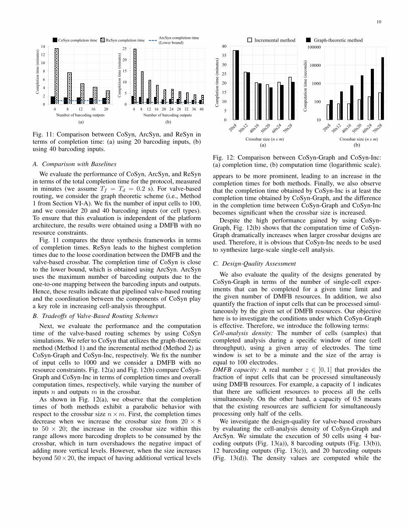
Fig. 11: Comparison between CoSyn, ArcSyn, and ReSyn interms of completion time: (a) using 20 barcoding inputs, (b)using 40 barcoding inputs.

A. Comparison with Baselines

We evaluate the performance of CoSyn, ArcSyn, and ReSynin terms of the total completion time for the protocol, measuredin minutes (we assume Tf = Td = 0.2 s). For valve-basedrouting, we consider the graph theoretic scheme (i.e., Method1 from Section VI-A). We fix the number of input cells to 100,and we consider 20 and 40 barcoding inputs (or cell types).To ensure that this evaluation is independent of the platformarchitecture, the results were obtained using a DMFB with noresource constraints.

Fig. 11 compares the three synthesis frameworks in termsof completion times. ReSyn leads to the highest completiontimes due to the loose coordination between the DMFB and thevalve-based crossbar. The completion time of CoSyn is closeto the lower bound, which is obtained using ArcSyn. ArcSynuses the maximum number of barcoding outputs due to theone-to-one mapping between the barcoding inputs and outputs.Hence, these results indicate that pipelined valve-based routingand the coordination between the components of CoSyn playa key role in increasing cell-analysis throughput.B. Tradeoffs of Valve-Based Routing Schemes

Next, we evaluate the performance and the computationtime of the valve-based routing schemes by using CoSynsimulations. We refer to CoSyn that utilizes the graph-theoreticmethod (Method 1) and the incremental method (Method 2) asCoSyn-Graph and CoSyn-Inc, respectively. We fix the numberof input cells to 1000 and we consider a DMFB with noresource constraints. Fig. 12(a) and Fig. 12(b) compare CoSyn-Graph and CoSyn-Inc in terms of completion times and overallcomputation times, respectively, while varying the number ofinputs n and outputs m in the crossbar.

As shown in Fig. 12(a), we observe that the completiontimes of both methods exhibit a parabolic behavior withrespect to the crossbar size n×m. First, the completion timesdecrease when we increase the crossbar size from 20 × 8to 50 × 20; the increase in the crossbar size within thisrange allows more barcoding droplets to be consumed by thecrossbar, which in turn overshadows the negative impact ofadding more vertical levels. However, when the size increasesbeyond 50×20, the impact of having additional vertical levels

(a) (b)

Incremental method Graph-theoretic method

0

5

10

15

20

25

30

35

40

Com

plet

ion

time

(min

utes

)

Crossbar size (n x m)

10

100

1000

10000

100000

Com

puta

tion

time

(sec

onds

)

Crossbar size (n x m)

Fig. 12: Comparison between CoSyn-Graph and CoSyn-Inc:(a) completion time, (b) computation time (logarithmic scale).

appears to be more prominent, leading to an increase in thecompletion times for both methods. Finally, we also observethat the completion time obtained by CoSyn-Inc is at least thecompletion time obtained by CoSyn-Graph, and the differencein the completion time between CoSyn-Graph and CoSyn-Incbecomes significant when the crossbar size is increased.

Despite the high performance gained by using CoSyn-Graph, Fig. 12(b) shows that the computation time of CoSyn-Graph dramatically increases when larger crossbar designs areused. Therefore, it is obvious that CoSyn-Inc needs to be usedto synthesize large-scale single-cell analysis.

C. Design-Quality Assessment

We also evaluate the quality of the designs generated byCoSyn-Graph in terms of the number of single-cell exper-iments that can be completed for a given time limit andthe given number of DMFB resources. In addition, we alsoquantify the fraction of input cells that can be processed simul-taneously by the given set of DMFB resources. Our objectivehere is to investigate the conditions under which CoSyn-Graphis effective. Therefore, we introduce the following terms:Cell-analysis density: The number of cells (samples) thatcompleted analysis during a specific window of time (cellthroughput), using a given array of electrodes. The timewindow is set to be a minute and the size of the array isequal to 100 electrodes.DMFB capacity: A real number z ∈ [0, 1] that provides thefraction of input cells that can be processed simultaneouslyusing DMFB resources. For example, a capacity of 1 indicatesthat there are sufficient resources to process all the cellssimultaneously. On the other hand, a capacity of 0.5 meansthat the existing resources are sufficient for simultaneouslyprocessing only half of the cells.

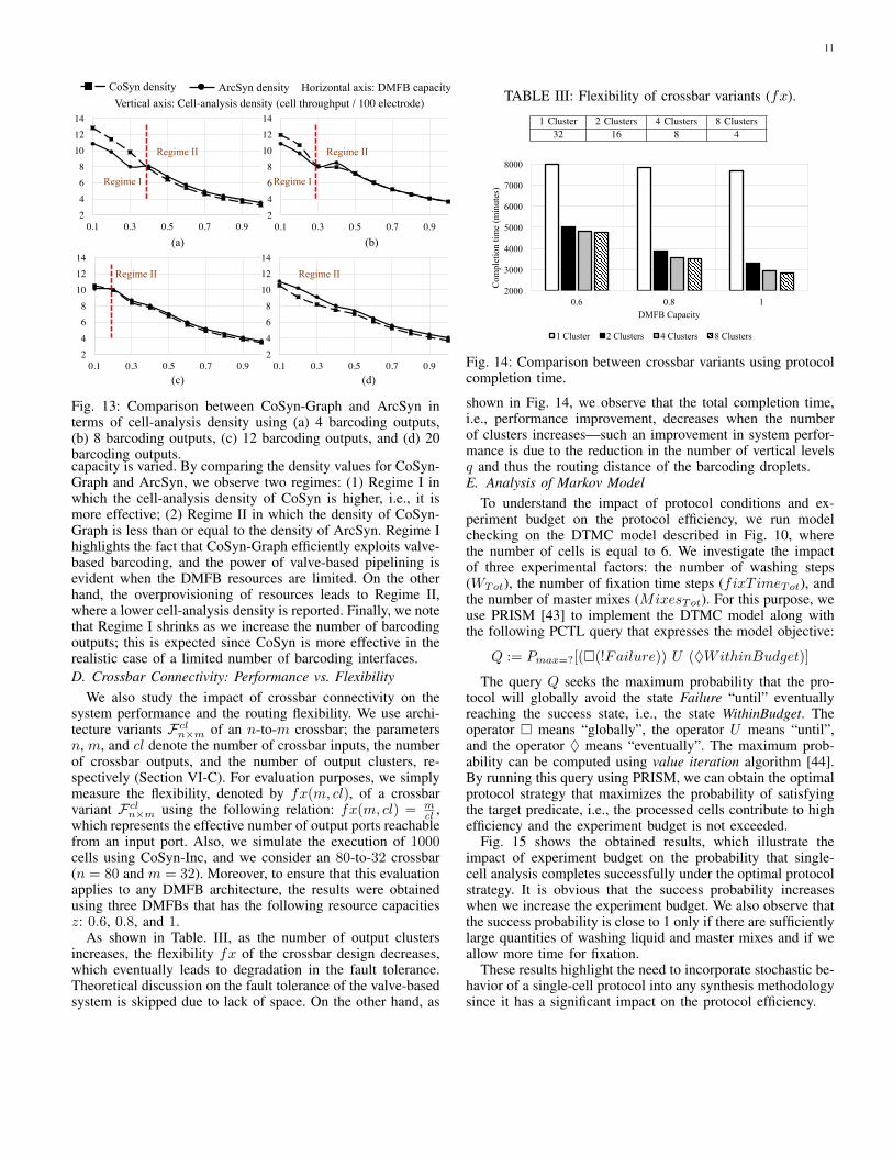
We investigate the design-quality for valve-based crossbarsby evaluating the cell-analysis density of CoSyn-Graph andArcSyn. We simulate the execution of 50 cells using 4 bar-coding outputs (Fig. 13(a)), 8 barcoding outputs (Fig. 13(b)),12 barcoding outputs (Fig. 13(c)), and 20 barcoding outputs(Fig. 13(d)). The density values are computed while the

11

2468

101214

0.1 0.3 0.5 0.7 0.9

CoSyn density ArcSyn density

Regime I

Regime II

(a) (b)

2468

101214

0.1 0.3 0.5 0.7 0.9

2468

101214

0.1 0.3 0.5 0.7 0.9

Horizontal axis: DMFB capacity

2468

101214

0.1 0.3 0.5 0.7 0.9

Regime II

Regime I

Regime II Regime II

(c) (d)

Vertical axis: Cell-analysis density (cell throughput / 100 electrode)

Fig. 13: Comparison between CoSyn-Graph and ArcSyn interms of cell-analysis density using (a) 4 barcoding outputs,(b) 8 barcoding outputs, (c) 12 barcoding outputs, and (d) 20barcoding outputs.capacity is varied. By comparing the density values for CoSyn-Graph and ArcSyn, we observe two regimes: (1) Regime I inwhich the cell-analysis density of CoSyn is higher, i.e., it ismore effective; (2) Regime II in which the density of CoSyn-Graph is less than or equal to the density of ArcSyn. Regime Ihighlights the fact that CoSyn-Graph efficiently exploits valve-based barcoding, and the power of valve-based pipelining isevident when the DMFB resources are limited. On the otherhand, the overprovisioning of resources leads to Regime II,where a lower cell-analysis density is reported. Finally, we notethat Regime I shrinks as we increase the number of barcodingoutputs; this is expected since CoSyn is more effective in therealistic case of a limited number of barcoding interfaces.D. Crossbar Connectivity: Performance vs. Flexibility

We also study the impact of crossbar connectivity on thesystem performance and the routing flexibility. We use archi-tecture variants Fcln×m of an n-to-m crossbar; the parametersn, m, and cl denote the number of crossbar inputs, the numberof crossbar outputs, and the number of output clusters, re-spectively (Section VI-C). For evaluation purposes, we simplymeasure the flexibility, denoted by fx(m, cl), of a crossbarvariant Fcln×m using the following relation: fx(m, cl) = m

cl ,which represents the effective number of output ports reachablefrom an input port. Also, we simulate the execution of 1000cells using CoSyn-Inc, and we consider an 80-to-32 crossbar(n = 80 and m = 32). Moreover, to ensure that this evaluationapplies to any DMFB architecture, the results were obtainedusing three DMFBs that has the following resource capacitiesz: 0.6, 0.8, and 1.

As shown in Table. III, as the number of output clustersincreases, the flexibility fx of the crossbar design decreases,which eventually leads to degradation in the fault tolerance.Theoretical discussion on the fault tolerance of the valve-basedsystem is skipped due to lack of space. On the other hand, as

TABLE III: Flexibility of crossbar variants (fx).

1 Cluster 2 Clusters 4 Clusters 8 Clusters32 16 8 4

2000

3000

4000

5000

6000

7000

8000

0.6 0.8 1

Com

plet

ion

time

(min

utes

)

DMFB Capacity

1 Cluster 2 Clusters 4 Clusters 8 Clusters

Fig. 14: Comparison between crossbar variants using protocolcompletion time.

shown in Fig. 14, we observe that the total completion time,i.e., performance improvement, decreases when the numberof clusters increases—such an improvement in system perfor-mance is due to the reduction in the number of vertical levelsq and thus the routing distance of the barcoding droplets.E. Analysis of Markov Model

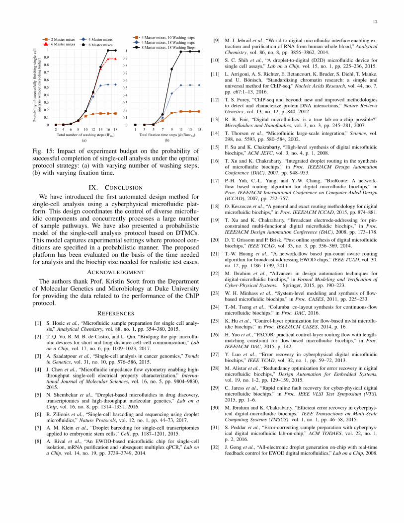
To understand the impact of protocol conditions and ex-periment budget on the protocol efficiency, we run modelchecking on the DTMC model described in Fig. 10, wherethe number of cells is equal to 6. We investigate the impactof three experimental factors: the number of washing steps(WTot), the number of fixation time steps (fixT imeTot), andthe number of master mixes (MixesTot). For this purpose, weuse PRISM [43] to implement the DTMC model along withthe following PCTL query that expresses the model objective:

Q := Pmax=?[(�(!Failure)) U (♦WithinBudget)]

The query Q seeks the maximum probability that the pro-tocol will globally avoid the state Failure “until” eventuallyreaching the success state, i.e., the state WithinBudget. Theoperator � means “globally”, the operator U means “until”,and the operator ♦ means “eventually”. The maximum prob-ability can be computed using value iteration algorithm [44].By running this query using PRISM, we can obtain the optimalprotocol strategy that maximizes the probability of satisfyingthe target predicate, i.e., the processed cells contribute to highefficiency and the experiment budget is not exceeded.

Fig. 15 shows the obtained results, which illustrate theimpact of experiment budget on the probability that single-cell analysis completes successfully under the optimal protocolstrategy. It is obvious that the success probability increaseswhen we increase the experiment budget. We also observe thatthe success probability is close to 1 only if there are sufficientlylarge quantities of washing liquid and master mixes and if weallow more time for fixation.

These results highlight the need to incorporate stochastic be-havior of a single-cell protocol into any synthesis methodologysince it has a significant impact on the protocol efficiency.

12

0

0.1

0.2

0.3

0.4

0.5

0.6

0.7

0.8

0.9

1

2 4 6 8 10 12 14 16 18

Prob

abili

ty o

f suc

cess

fully

fini

shin

g si

ngle

-cel

l an

alys

is w

ithou

t exc

eedi

ng b

udge

t

Total number of washing steps (WTot)

2 Master mixes 4 Master mixes8 Master mixes6 Master mixes

(a)

0

0.1

0.2

0.3

0.4

0.5

0.6

0.7

0.8

0.9

1

1 3 5 7 9 11 13 15Total fixation time steps (fixTimeTot)

(b)

4 Master mixes, 10 Washing steps4 Master mixes, 18 Washing steps8 Master mixes, 18 Washing Steps

Fig. 15: Impact of experiment budget on the probability ofsuccessful completion of single-cell analysis under the optimalprotocol strategy: (a) with varying number of washing steps;(b) with varying fixation time.

IX. CONCLUSION

We have introduced the first automated design method forsingle-cell analysis using a cyberphysical microfluidic plat-form. This design coordinates the control of diverse microflu-idic components and concurrently processes a large numberof sample pathways. We have also presented a probabilisticmodel of the single-cell analysis protocol based on DTMCs.This model captures experimental settings where protocol con-ditions are specified in a probabilistic manner. The proposedplatform has been evaluated on the basis of the time neededfor analysis and the biochip size needed for realistic test cases.

ACKNOWLEDGMENT

The authors thank Prof. Kristin Scott from the Departmentof Molecular Genetics and Microbiology at Duke Universityfor providing the data related to the performance of the ChIPprotocol.

REFERENCES

[1] S. Hosic et al., “Microfluidic sample preparation for single cell analy-sis,” Analytical Chemistry, vol. 88, no. 1, pp. 354–380, 2015.

[2] T. Q. Vu, R. M. B. de Castro, and L. Qin, “Bridging the gap: microflu-idic devices for short and long distance cell–cell communication,” Labon a Chip, vol. 17, no. 6, pp. 1009–1023, 2017.

[3] A. Saadatpour et al., “Single-cell analysis in cancer genomics,” Trendsin Genetics, vol. 31, no. 10, pp. 576–586, 2015.

[4] J. Chen et al., “Microfluidic impedance flow cytometry enabling high-throughput single-cell electrical property characterization,” Interna-tional Journal of Molecular Sciences, vol. 16, no. 5, pp. 9804–9830,2015.

[5] N. Shembekar et al., “Droplet-based microfluidics in drug discovery,transcriptomics and high-throughput molecular genetics,” Lab on aChip, vol. 16, no. 8, pp. 1314–1331, 2016.

[6] R. Zilionis et al., “Single-cell barcoding and sequencing using dropletmicrofluidics,” Nature Protocols, vol. 12, no. 1, pp. 44–73, 2017.

[7] A. M. Klein et al., “Droplet barcoding for single-cell transcriptomicsapplied to embryonic stem cells,” Cell, pp. 1187–1201, 2015.

[8] A. Rival et al., “An EWOD-based microfluidic chip for single-cellisolation, mRNA purification and subsequent multiplex qPCR,” Lab ona Chip, vol. 14, no. 19, pp. 3739–3749, 2014.

[9] M. J. Jebrail et al., “World-to-digital-microfluidic interface enabling ex-traction and purification of RNA from human whole blood,” AnalyticalChemistry, vol. 86, no. 8, pp. 3856–3862, 2014.

[10] S. C. Shih et al., “A droplet-to-digital (D2D) microfluidic device forsingle cell assays,” Lab on a Chip, vol. 15, no. 1, pp. 225–236, 2015.

[11] L. Arrigoni, A. S. Richter, E. Betancourt, K. Bruder, S. Diehl, T. Manke,and U. Bonisch, “Standardizing chromatin research: a simple anduniversal method for ChIP-seq,” Nucleic Acids Research, vol. 44, no. 7,pp. e67:1–13, 2016.

[12] T. S. Furey, “ChIP-seq and beyond: new and improved methodologiesto detect and characterize protein-DNA interactions,” Nature ReviewsGenetics, vol. 13, no. 12, p. 840, 2012.

[13] R. B. Fair, “Digital microfluidics: is a true lab-on-a-chip possible?”Microfluidics and Nanofluidics, vol. 3, no. 3, pp. 245–281, 2007.

[14] T. Thorsen et al., “Microfluidic large-scale integration,” Science, vol.298, no. 5593, pp. 580–584, 2002.

[15] F. Su and K. Chakrabarty, “High-level synthesis of digital microfluidicbiochips,” ACM JETC, vol. 3, no. 4, p. 1, 2008.

[16] T. Xu and K. Chakrabarty, “Integrated droplet routing in the synthesisof microfluidic biochips,” in Proc. IEEE/ACM Design AutomationConference (DAC), 2007, pp. 948–953.

[17] P.-H. Yuh, C.-L. Yang, and Y.-W. Chang, “BioRoute: A network-flow based routing algorithm for digital microfluidic biochips,” inProc. IEEE/ACM International Conference on Computer-Aided Design(ICCAD), 2007, pp. 752–757.

[18] O. Keszocze et al., “A general and exact routing methodology for digitalmicrofluidic biochips,” in Proc. IEEE/ACM ICCAD, 2015, pp. 874–881.

[19] T. Xu and K. Chakrabarty, “Broadcast electrode-addressing for pin-constrained multi-functional digital microfluidic biochips,” in Proc.IEEE/ACM Design Automation Conference (DAC), 2008, pp. 173–178.

[20] D. T. Grissom and P. Brisk, “Fast online synthesis of digital microfluidicbiochips,” IEEE TCAD, vol. 33, no. 3, pp. 356–369, 2014.

[21] T.-W. Huang et al., “A network-flow based pin-count aware routingalgorithm for broadcast-addressing EWOD chips,” IEEE TCAD, vol. 30,no. 12, pp. 1786–1799, 2011.

[22] M. Ibrahim et al., “Advances in design automation techniques fordigital-microfluidic biochips,” in Formal Modeling and Verification ofCyber-Physical Systems. Springer, 2015, pp. 190–223.

[23] W. H. Minhass et al., “System-level modeling and synthesis of flow-based microfluidic biochips,” in Proc. CASES, 2011, pp. 225–233.

[24] T.-M. Tseng et al., “Columba: co-layout synthesis for continuous-flowmicrofluidic biochips,” in Proc. DAC, 2016.

[25] K. Hu et al., “Control-layer optimization for flow-based mvlsi microflu-idic biochips,” in Proc. IEEE/ACM CASES, 2014, p. 16.

[26] H. Yao et al., “PACOR: practical control-layer routing flow with length-matching constraint for flow-based microfluidic biochips,” in Proc.IEEE/ACM DAC, 2015, p. 142.

[27] Y. Luo et al., “Error recovery in cyberphysical digital microfluidicbiochips,” IEEE TCAD, vol. 32, no. 1, pp. 59–72, 2013.

[28] M. Alistar et al., “Redundancy optimization for error recovery in digitalmicrofluidic biochips,” Design Automation for Embedded Systems,vol. 19, no. 1-2, pp. 129–159, 2015.

[29] C. Jaress et al., “Rapid online fault recovery for cyber-physical digitalmicrofluidic biochips,” in Proc. IEEE VLSI Test Symposium (VTS),2015, pp. 1–6.

[30] M. Ibrahim and K. Chakrabarty, “Efficient error recovery in cyberphys-ical digital-microfluidic biochips,” IEEE Transactions on Multi-ScaleComputing Systems (TMSCS), vol. 1, no. 1, pp. 46–58, 2015.

[31] S. Poddar et al., “Error-correcting sample preparation with cyberphys-ical digital microfluidic lab-on-chip,” ACM TODAES, vol. 22, no. 1,p. 2, 2016.

[32] J. Gong et al., “All-electronic droplet generation on-chip with real-timefeedback control for EWOD digital microfluidics,” Lab on a Chip, 2008.

13

i1i2

i3

i4

i5i6

i7

i8

in-1

in

o1o2

o3

o4

o5o6

om-1

om

i1

i2

i3

i4

i5

i6

in-1

in

o1

o2

om-1

om

q

s

(a) (b)

Box B(2,2)

Box B(s,s)

Horizontal level

Transposery

x

(0,0)

w1

w2

w2

Fig. 16: (a) A schematic view of an n-to-m routing crossbar; (b) the associated graph model F(n×m,T ).

[33] Y. Luo et al., “Design and optimization of a cyberphysical digital-microfluidic biochip for the polymerase chain reaction,” IEEE TCAD,vol. 34, no. 1, pp. 29–42, 2015.

[34] M. Ibrahim et al., “Synthesis of cyberphysical digital-microfluidicbiochips for real-time quantitative analysis,” IEEE Transactions onComputer-Aided Design of Integrated Circuits and Systems (TCAD),vol. 36, no. 5, pp. 733–746, 2017.

[35] M. Ibrahim et al., “A real-time digital-microfluidic platform for epige-netics,” in Proc. IEEE/ACM CASES, 2016, p. 10.

[36] S. Gomez, A. Arenas, J. Borge-Holthoefer, S. Meloni, and Y. Moreno,“Discrete-time markov chain approach to contact-based disease spread-ing in complex networks,” EPL (Europhysics Letters), vol. 89, no. 3, p.38009, 2010.

[37] C. Baier, J.-P. Katoen, and K. G. Larsen, Principles of model checking,2008.

[38] M. Kwiatkowska, “Quantitative verification: models techniques andtools,” in Proc. 6th joint meeting of the European Software EngineeringConference and the ACM SIGSOFT Symposium on the Foundations ofSoftware Engineering (ESEC/FSE), 2007, pp. 449–458.

[39] M. A. Murran and H. Najjaran, “Capacitance-based droplet positionestimator for digital microfluidic devices,” Lab on a Chip, 2012.

[40] M. Ibrahim et al., “Integrated and real-time quantitative analysis usingcyberphysical digital-microfluidic biochips,” in Proc. DATE, 2016.

[41] R. Silva et al., “A reconfigurable continuous-flow fluidic routing fabricusing a modular, scalable primitive,” Lab on a Chip, 2016.

[42] T. Cormen et al., Introduction to Algorithms. MIT Press Cambridge,2001.

[43] M. Kwiatkowska, G. Norman, and D. Parker, “PRISM 4.0: Verificationof probabilistic real-time systems,” in Computer Aided Verification.Springer, 2011, pp. 585–591.

[44] T. Chen, V. Forejt, M. Kwiatkowska, D. Parker, and A. Simaitis,“Automatic verification of competitive stochastic systems,” FormalMethods in System Design, vol. 43, no. 1, pp. 61–92, 2013.

APPENDIX APROOF OF THEOREM 1: A FULLY CONNECTED ROUTING

CROSSBAR

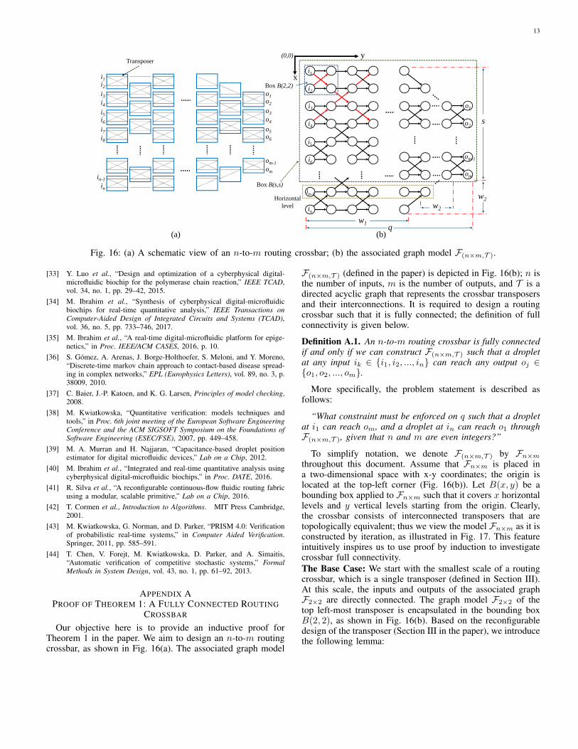
Our objective here is to provide an inductive proof forTheorem 1 in the paper. We aim to design an n-to-m routingcrossbar, as shown in Fig. 16(a). The associated graph model

F(n×m,T ) (defined in the paper) is depicted in Fig. 16(b); n isthe number of inputs, m is the number of outputs, and T is adirected acyclic graph that represents the crossbar transposersand their interconnections. It is required to design a routingcrossbar such that it is fully connected; the definition of fullconnectivity is given below.

Definition A.1. An n-to-m routing crossbar is fully connectedif and only if we can construct F(n×m,T ) such that a dropletat any input ik ∈ {i1, i2, ..., in} can reach any output oj ∈{o1, o2, ..., om}.

More specifically, the problem statement is described asfollows:

“What constraint must be enforced on q such that a dropletat i1 can reach om, and a droplet at in can reach o1 throughF(n×m,T ), given that n and m are even integers?”

To simplify notation, we denote F(n×m,T ) by Fn×mthroughout this document. Assume that Fn×m is placed ina two-dimensional space with x-y coordinates; the origin islocated at the top-left corner (Fig. 16(b)). Let B(x, y) be abounding box applied to Fn×m such that it covers x horizontallevels and y vertical levels starting from the origin. Clearly,the crossbar consists of interconnected transposers that aretopologically equivalent; thus we view the model Fn×m as it isconstructed by iteration, as illustrated in Fig. 17. This featureintuitively inspires us to use proof by induction to investigatecrossbar full connectivity.The Base Case: We start with the smallest scale of a routingcrossbar, which is a single transposer (defined in Section III).At this scale, the inputs and outputs of the associated graphF2×2 are directly connected. The graph model F2×2 of thetop left-most transposer is encapsulated in the bounding boxB(2, 2), as shown in Fig. 16(b). Based on the reconfigurabledesign of the transposer (Section III in the paper), we introducethe following lemma:

14

i1

i2

i3

i4

Iteration 1

Iteration 2

Iteration p

Iteration 1 Iteration 2 Iteration p(a)

(b)

Fig. 17: Iterative construction of an Fn×m.

i1

i2

ik+1

ik+2 ok+2

ok+1

ik

i1

(a)

T3 T2

T1ok

P3 P2

P1

Black box

o1

i1

i2

ok

ok-1

ik

i1

(b)

T2

T1

ok

o1

o1

Fig. 18: Expanding the graph model Fk×k to (a) F(k+2)×(k+2),(b) Fk×(k+2).

Lemma A.1. A full (half) transposer is a 2-to-2 (2-to-1) fullyconnected crossbar.

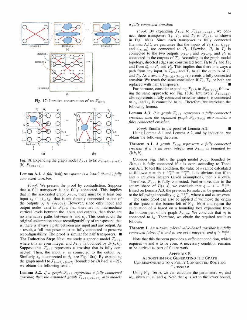
Proof: We present the proof by contradiction. Supposethat a full transposer is not fully connected. This impliesthat in the associated graph F2×2, there must be at least oneinput ik ∈ {i1, i2} that is not directly connected to one ofthe outputs oj ∈ {o1, o2}. However, since only input andoutput nodes exist in F2×2, i.e., there are no intermediatevertical levels between the inputs and outputs, then there areno alternative paths between ik and oj . This contradicts theoriginal assumption about reconfigurability of transposers; thatis, there is always a path between any input and any output. Asa result, a full transposer must be fully connected to preservereconfigurability. The proof is similar for half transposers.The Induction Step: Next, we study a generic model Fk×k,where k is an even integer, and Fk×k is bounded by B(k, k).Suppose that Fk×k represents a crossbar that is fully con-nected. Then, the input i1 is connected to the output ok.Similarly, ik is connected to o1; see Fig. 18(a). By expandingthe graph model to F(k+2)×(k+2) (bounded by B(k+2, k+2)),we obtain the following result.

Lemma A.2. If a graph Fk×k represents a fully connectedcrossbar, then the expanded graph F(k+2)×(k+2) also models

a fully connected crossbar.

Proof: By expanding Fk×k to F(k+2)×(k+2), we con-nect three transposers T1, T2, and T3 to Fk×k, as shownin Fig. 18(a). Since each transposer is fully connected(Lemma A.1), we guarantee that the inputs of T3 (i.e., i(k+1)

and i(k+2)) are connected to P3. Likewise, P2 in T2 isconnected to the two outputs o(k+1) and o(k+2), and P1 isconnected to the outputs of T1. According to the graph modeltopology, directed edges are constructed from P3 to P1 and P2,and from ok to P1 and P2. This implies that there is always apath from any input in Fk×k and T3 to all the outputs of T1and T2. As a result, F(k+2)×(k+2) represents a fully connectedcrossbar. We reach the same conclusion if T1, T2, or both arereplaced with half transposers.

Furthermore, consider expanding Fk×k to Fk×(k+2) follow-ing the same approach; see Fig. 18(b). Intuitively, Fk×(k+2)

also represents a fully connected crossbar, since i1 is connectedto ok, and ik is connected to o1. Therefore, we introduce thefollowing lemma.

Lemma A.3. If a graph Fk×k represents a fully connectedcrossbar, then the expanded graph Fk×(k+2) also models afully connected crossbar.

Proof: Similar to the proof of Lemma A.2.Using Lemma A.1 and Lemma A.2, and by induction, we

obtain the following theorem.

Theorem A.1. A graph Fk×k represents a fully connectedcrossbar if k is an even integer and Fk×k is bounded byB(k, k).

Consider Fig. 16(b), the graph model Fs×s bounded byB(s, s) is fully connected if s is even, according to Theo-rem A.1. To test this condition, the value of s can be calculatedas follows: s = m + n−m

2 = n+m2 . It is obvious that if m

and n are even integers (given assumption), then s is even.Therefore, Fs×s is fully connected. Furthermore, due to thesquare shape of B(s, s), we conclude that q = s = n+m

2 .Based on Lemma A.3, the previous formula can be generalizedto the following inequality: q ≥ n+m

2 , where n and m are even.The same proof can also be applied if we move the origin

of the space to the bottom left of Fig. 16(b) and repeat thecalculation of q based on a bounding box expanding fromthe bottom part of the graph Fn×m. We conclude that o1 isconnected to in. Therefore, we obtain the required result asfollows.

Theorem 1. An n-to-m, q-level valve-based crossbar is a fullyconnected fabric if n and m are even integers, and q ≥ m+n

2 .

Note that this theorem provides a sufficient condition, whichrequires m and n to be even. A necessary condition remainsto be derived as part of future work.

APPENDIX BALGORITHM FOR GENERATING THE GRAPH

CORRESPONDING TO A FULLY CONNECTED ROUTINGCROSSBAR

Using Fig. 16(b), we can calculate the parameters w1 andw2, given m, n, and q. Note that q is set to the lower bound,

15

w1 = 5

w2=2

i1

q = 8

i2

i3

i4

i5

i6

i7

i8

i9

i10

o1

o2

o3

o4

o5

o6

Line (3)

Lines (5-13)

Lines (15-24)

Lines (26-31)

Fig. 19: The application of Algorithm 3 on a graph F10×6.

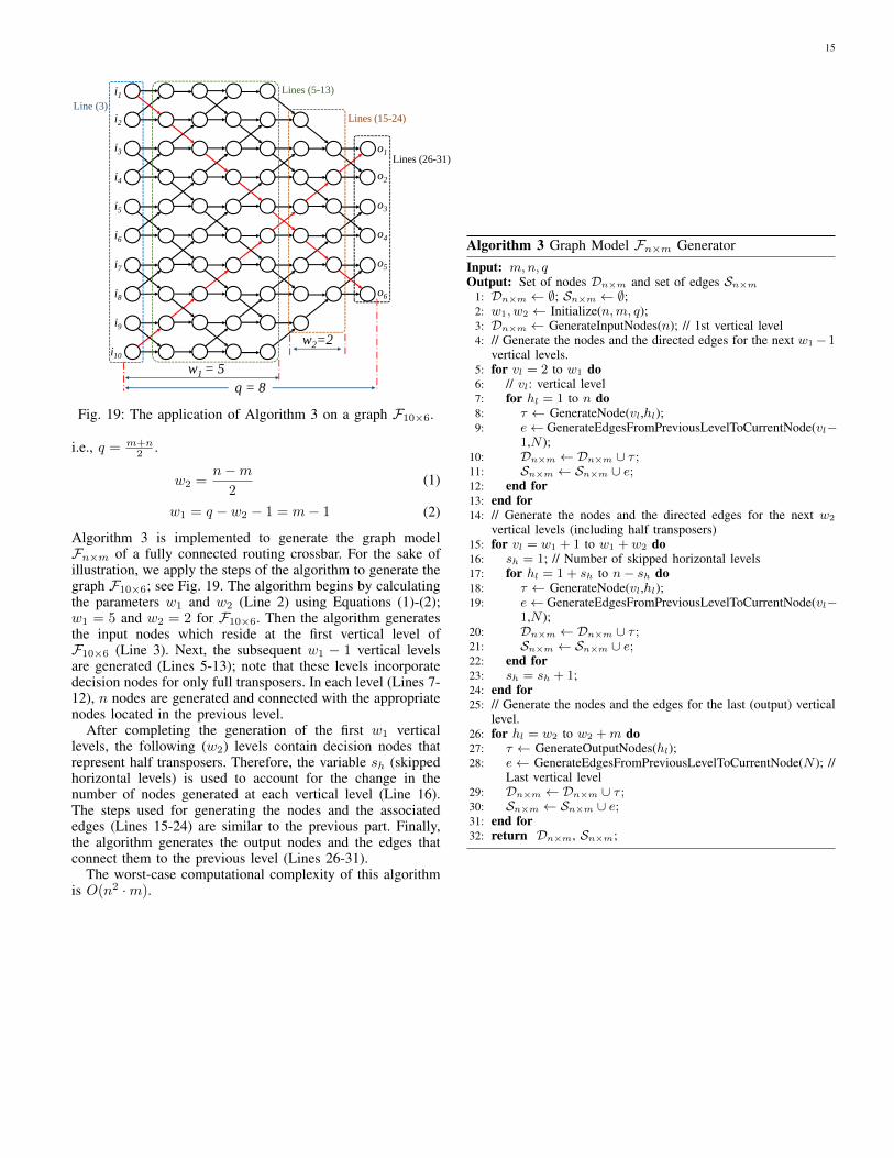
i.e., q = m+n2 .

w2 =n−m

2(1)

w1 = q − w2 − 1 = m− 1 (2)

Algorithm 3 is implemented to generate the graph modelFn×m of a fully connected routing crossbar. For the sake ofillustration, we apply the steps of the algorithm to generate thegraph F10×6; see Fig. 19. The algorithm begins by calculatingthe parameters w1 and w2 (Line 2) using Equations (1)-(2);w1 = 5 and w2 = 2 for F10×6. Then the algorithm generatesthe input nodes which reside at the first vertical level ofF10×6 (Line 3). Next, the subsequent w1 − 1 vertical levelsare generated (Lines 5-13); note that these levels incorporatedecision nodes for only full transposers. In each level (Lines 7-12), n nodes are generated and connected with the appropriatenodes located in the previous level.

After completing the generation of the first w1 verticallevels, the following (w2) levels contain decision nodes thatrepresent half transposers. Therefore, the variable sh (skippedhorizontal levels) is used to account for the change in thenumber of nodes generated at each vertical level (Line 16).The steps used for generating the nodes and the associatededges (Lines 15-24) are similar to the previous part. Finally,the algorithm generates the output nodes and the edges thatconnect them to the previous level (Lines 26-31).

The worst-case computational complexity of this algorithmis O(n2 ·m).

Algorithm 3 Graph Model Fn×m GeneratorInput: m,n, qOutput: Set of nodes Dn×m and set of edges Sn×m

1: Dn×m ← ∅; Sn×m ← ∅;2: w1, w2 ← Initialize(n,m, q);3: Dn×m ← GenerateInputNodes(n); // 1st vertical level4: // Generate the nodes and the directed edges for the next w1− 1

vertical levels.5: for vl = 2 to w1 do6: // vl: vertical level7: for hl = 1 to n do8: τ ← GenerateNode(vl,hl);9: e← GenerateEdgesFromPreviousLevelToCurrentNode(vl−

1,N );10: Dn×m ← Dn×m ∪ τ ;11: Sn×m ← Sn×m ∪ e;12: end for13: end for14: // Generate the nodes and the directed edges for the next w2

vertical levels (including half transposers)15: for vl = w1 + 1 to w1 + w2 do16: sh = 1; // Number of skipped horizontal levels17: for hl = 1 + sh to n− sh do18: τ ← GenerateNode(vl,hl);19: e← GenerateEdgesFromPreviousLevelToCurrentNode(vl−

1,N );20: Dn×m ← Dn×m ∪ τ ;21: Sn×m ← Sn×m ∪ e;22: end for23: sh = sh + 1;24: end for25: // Generate the nodes and the edges for the last (output) vertical

level.26: for hl = w2 to w2 +m do27: τ ← GenerateOutputNodes(hl);28: e← GenerateEdgesFromPreviousLevelToCurrentNode(N ); //

Last vertical level29: Dn×m ← Dn×m ∪ τ ;30: Sn×m ← Sn×m ∪ e;31: end for32: return Dn×m, Sn×m;