1 SystemsOptimization

' Laboratory

LC)0

Primal Barrier Methods For Linear Programming

byAeneas Marxen

TECHNICAL REPORT SOL 89-6

June 1989

DTIC

JUL 89

Department of Operations ResearchStanford UniversityStanford, CA 94305

89 7 44 081

SYSTEMS OPTIMIZATION LABORATORYDEPARTMENT OF OPERATIONS RESEARCH

STANFORD UNIVERSITYSTANFORD, CALIFORNIA 94305-4022

Primal Barrier Methods For Linear Programming

byAeneas Marxen

TECHNICAL REPORT SOL 89-6

June 1989

Research and reproduction of this report were partially supported by the U.S. Department of EnergyGrant DE-FG03-87ER25030, and Office of Naval Research Contract N00014-87-K-0142.

Any opinions, findings, and conclusions or recommendations expressed in this publication are thoseof the author and do NOT necessarily reflect the views of the above sponsors.

Reproduction in whole or in part is permitted for any purposes of the United States Government.This document has been approved for public release and sale; its distribution is unlimited.

DT1C

S JL I

FEgC j JJUJL 9 4 199

E

PRIMAL BARRIER METHODS FOR LINEAR PROGRAMMING

Aeneas Marxen, Ph.D.

Stanford University, 1989

The linear program rin cTx subject to Ax = b, x > 0, is solved by the ,roj('(I( .\tion

barrier method. The method consists of solving a sequence of subproblenis of the form

nin cTx-p in xj subject to Ax = b. Extensions for upper bounds, free and fixed vari~lbles

are given. A linear modification is made to the logarithmic barrier function, which results

in the solution being bounded in all cases. It also facilitates the provisiou of a good startinig

point. The solution of each subproblem involves repeatedly conl)utin~g a sarch dir,,ctin

and taking a step along this direction. Ways to find an initial feasib.,. soluti,,i..S( 1) "izS

and convergence criteria are discussed.

Like other interior-point method for linear programming, this method solves a systim of

the form AH-'4 .- y, where H is diagonal. This system can be very ill-comditioiied aid

special precautions must be taken for the Cholesky factorization. The matrix A is assumed

to be large and sparse. Data structures and algorithms for the sparse factorizatiotl are

explained. In particular, the consequences of relatively dense columns in A are investigated

and a Schur-complement method is introduced to maintain the speed of the method in these

cases.

An implementation of the method was developed as part of the rese;r'ch. Results of ex-

tensive testing with medium to large problems are presented and the testinig methodologies

used are discussed. Aoesson or

NTIS GRA&ID TL i -n

D u st rI.- t Ic:( .. Jtsti±- tc:L/

Avail,.Il ity Codes

-4 Avo, ' 1 ,,ad/orDist Sp,;cIal

S'l- .

Gewidniet meinen Eltern,

Gisela und Aeneas Marxen,

deren Liebe, Grofizigigkeit und Ermutigung

ich alles zu verdan ken babe.

Introduction

From the beginning, linear programming problems have played a central role iii ()per;,ii.,

Research. Discovered by George B. Dantzig in 1947, the sinplex Inethod iii its Iiiialiv

variations has evolved as the standard algorithm for linear programming. For a lilear

program (LP) that has a solution, there usually exists an optimal point at a velrtx of lie

feasible region. The iterates of the simplex method move along the bouidary of tile feasible

region to find such a vertex. The simplex method can be shown to require a non-polytomiial

number of iterations for a contrived class of problems, although in practice it tellds to lleed

a number of iterations that is little more than linear in the )roblem dimnieiiojis.

A number of alternatives to the simplex method that generate iterates in the intcrior

of the feasible region, were proposed early on. Among them was the barrier lilethod. (For

a complete discussion of barrier methods, see Fiacco [Fia79]. Classical barrier ald t)elalty

methods are described in Fiacco and McCormick [FM681. Fletcher [FleS] and Gill, NlIirrav

and Wright [GMW81] give overviews of barrier and penalty methods.) The logarithmic

barrier function considered in this thesis was first suggested by Frisch [Fri54,57]. It was

utilized to devise a sequence of nonlinear, unconstrained subproblems for solviiic- linear

programs by Parisot [Par6l]. Osborne [Osb72] and Wright [Wri76] added an active set

strategy to the method, an idea not followed in this research. Gill et al. [(MST\VS(i]

proposed using Newton's method to solve individual subproblems.

Although the number of subproblems has been observed to be small, the lnonlilleari-

ties involved make them hard problems to solve. Additionally there is a, certain niiniiminmn

number of subproblems, irrespective of problem size. Since at the outset the olly prob-

lems solved were small by today's standards, the barrier method was not coiisidere(l to

be competitive with the simplex method at that time. Interest revived receitly, however.

when improvements in design and performance of computers and improved algorithms for

factorizing sparse matrices made interior-point methods an alternative worthy of serious

consideration.

The spark for this renewed interest came when Karmarkar [Kar84] demnmistrated that

the combinatorial complexity of finding the optimal vertex can be overcomie by solviig a

4

series of nonlinear optimization problems whose optimal point is interior. Subsequently it

was shown that tile algorithm he used is closely related to one proposed by 1)ikin [I)ik671.

The theoretical question, whether a linear programming algorithm with only polynomial

complexity can be found, had been resolved earlier when Khachiyan [Kha79] analysed his

method based on an algorithm of shrinking ellipsoids [Shor77].

It is now generally recognized that essentially all interior-point methods for linear pro-

gramming inspired by Karmarkar's projective method are closely related to application of

Newton's method to a sequence of barrier functions (see [GMSTW861). Newton's mothod

is based on minimizing a local quadratic model of the barrier function derived from first

and second derivative information at the current iterate. Unfortunately, several difficulties

can arise because of the nature of barrier functions. The extreme nonlinearity of the barrier

term near the boundary means that a quadratic model may be accurate only in a very small

neighborhood of the current point. For a degenerate linear program, the system of e(lqa-

tions that has to be solved becomes increasingly ill-conditioned. Finally, the strictly interior

starting point that this method requires, may be inconvenient or impossible to obtain.

Recent publications (e.g. [ARV86], [MM87], [VMF86]) compare implementations of

interior-point methods to one of the simplex method and show impressive reductions in

computing time for a certain set of problems. However, there has been little interest in

comparing different interior-point methods, and hardly any evidence is given concerning

their reliability. While interior-point methods seem similar enough that their comparison

can be safely left for future research, the issue of reliability is an important one. The ques-

tion of whether interior-point methods are fit to serve as an all-purpose replacement of the

simplex method for general linear programs, remains unanswered.

The intention of the research presented in this dissertation is to explore the behavior

of the barrier method when solving real-world, medium-to-large problems and to develop

ways of overcoming the obstacles encountered. As a general guideline, we have attempted

to develop the fastest algorithm that would be able to deal with the numerical difficulties

arising from degeneracy, rank-deficiency and other characteristics that make real-world

problems hard to solve. More importantly, we have tried to identify those areas where a

trade-off between speed and reliability must be made. The test set consists of the first 53

problems of the netlib collection [Gay85], which was formed as a benchmark for comparing

linear programming algorithms. At the outset of this research, no complete set of results

for these problems had been published for the new class of interior-point methods.

To make comparisons with the simplex method as meaningful as possible, an inmplemen-

tation was developed that operates under the same conditions as the simplex code to which

5

it was compared. In particular, both implementations work with the same constraint ma-

trix, require about the same amount of memory and were produced using the same portable,

high-level computer language. No assessment is made of whether enhancements in any of

these three directions might benefit one method more than the other.

I have been privileged in that I was able to conduct this research in close collaboration

with the SOL Algorithms Group in the Operations Research Department at Stanford. The

discussions in tGe group and the extensive support I received from the associated researchers

and students were very helpful. I would like to thank Prof. George B. Dantzig for serving

on my doctoral committee, for two most interesting research seminars, and for giving me

a perspective on the evolution of the field. Margaret H. Wright became important for

this thesis almost unintentionally; she gave a lively and fascinating presentation on barrier

methods for LP as part of the OR Colloquium series, and she provided an office with a

computer workstation by being on leave throughout 1988. I am indebted to Prof. Michael

A. Saunders for sharing his experience and answering many questions, often late at night, as

well as for providing the MINOS subroutines. My thesis advisor, Prof. Walter Murray, will be

fondly remembered for his many invaluable suggestions, his humor and his generosity with

signatures for all my forms. And last, but not least, I would like to thank Prof. Philip E. Gill

for his time, patience and availability when helping me with my questions. References to

"P. E. Gill (1987, 1988). Private communication." were omitted from this manuscript, since

they might have rendered certain parts all but unreadable. If this dissertation turns out to

be readable and helpful, it is largely owing to his proofreading, whereas the idiosyncracies

and shortcomings are solely mine.

A. Mx.

6

Part I The Algorithm

Chapter 1

What is the problem ?

The linear program considered is of the following standard form:

SLP minimize cTx

subject to Ax = b

X >0.

The vector x E R' contains the decision variables, c E R ' contains the weights of the

objective function. The matrix A E ,xn is called the constraint matrix and is assumed

to be of full row rank. The vector b E Rm is called the right-hand side. The feasible region

of the problem is assumed to have a nonempty interior, so that there exists an x such that

Ax=b and x>0.

The constraint matrices of the problems to be considered are large (up to 10000 columns)

and very sparse (90%-99% of the elements are zero).

We want to find a solution x * of this problem by solving a sequence k = 1,2,...

of barrier-function subproblems. Here, the nonnegativity constraints are no longer stated

explicitly, but are enforced implicitly by the objective function. A barrier subproblem is of

the form

minimize Fk(x) CTi +)

subject to Ax = b.

With the proper choice of Fk(x), the sequence of solutions x*(k) of these subproblems

converges to the solution x* of the original problem.

Since a second-derivative method is used to solve each subproblem, wo shall define

g(x) = VF(x) and H(x) = V 2 F(x) to be the gradient and the Hessian of the objective

7

function. (The subproblem index k is omitted for clarity, unless needed.) We denote

9 = c+ g, 9Bj = Ofoxj

and

H = diagh, hj=@2f3 /OX2, j= 1,...,n.

The functions fj are defined to be strictly convex over the interior of the feasible region,

so that hj > 0 for all j and H 1 exists. Note that F(x) is separable so that the Hessian

H is a diagonal matrix and its inverse H- 1 is readily computable as

f1-1 = diag (1/hI,..., 1/h,).

The Lagrangian function associated with the subproblem is F(x) - 7rT(Ax - b), where

7rb denotes the Lagrange multipliers of the constraints Ax = b. The first-order necessary

condition for optimality is that the gradient of the Lagrangian at x*(k) must vanish, i.e.,

g- ATrb = 0.

The Projected Newton Method

To solve the subproblcm, a feasible-point descent method is employed. Every iterate x

satisfies the constraints Ax = b, and the next point x' is found on a search direction p,

so that x' = x + ap. Convergence is ensured by choosing p as a descent direction, and a

such that the objective function value F(x') is sufficiently smaller than F(x) (see page 12).

Feasibility is ensured by satisfying Ax ° = b for the initial point and the null-space condition

Ap = 0.

The Newton search direction satisfies these conditions and is computed using second-

derivative information. The direction is defined as the step to the minimizer of a quadratic

approximation to F(x) on the feasible region, as derived from the local Taylor series. Thus

p is the solution of the quadratic program

minimize gTp 2 p Hpp

subject to Ap = 0.

The vcctor p satisfies the QP-optimality condition

g + Hp- ATir = 0,

8

where .r is the vector of Lagrange multipliers associated with the equality constraints

Ap = 0. Since p - 0 as x - x*(k), the Lagrange multipliers ir converge to the

multipliers 7r6 of the original problem.

Note that p = 0 is feasible for the QP, so that the optimal objective function value is

not positive and gTp < -L THp < 0 for the optimal p.

The null-space condition and the QP-optimality condition can be summarized in the

Karush- Kuhn- Tucker (K KT) system,H: AT -: ) o .In our implementation, the KKT-system is solved by computing 7r from the positive-definite

system

Ai- ATr = AI- 1g,

and by recovering the search direction as p = t- 1 (g - ATr).

These equations are called normal equations, a name taken from a weighted least-squares

problem that is equivalent to the KKT-system. Let D be a diagonal matrix such that

D' = I - I and define a vector r = -D-Ip. Now r and 7r satisfy

( I DAT (r>(Dg)AD T z 0

so that 7r is the solution, and r the optimal residual, of

minimize JID(g - aT r)112.

Flie derivative of this norm with respect to 7r is 2AD 2 ATr - 2AD 2g. Solving for the zero

of this derivative gives the normal equations.

The solution of the KKT-system is by far the most difficult aspect of using an interior-

point method, both in terms of computational effort and in terms of numerical problenis

that must be dealt with. Exploiting sparsity in A is essential for the efficiency of the

whole algorithm, and finding a way to deal with ill-conditioning in A and H is crucial for

reliability. Part I1 will be devoted to these difficulties. For the rest of Part I we assume

that a search direction p can always be computed.

The Newton stel from x to x' = x + ap is sometimes referred to as a minor itc'ra-

tion. This is to distinguish it from a major iteration, which is the solution of one barrier

subproblem. Unless stated otherwise, we will use the term iterations to refer to minor

iterations.

9

The Logarithmic Barrier Function

A straightforward example of an objective function I'k(x) is the logarithmic barrier func-

t;on. The sequence of subproblems with decreasing barrier parameters it is defined as

minimize Frk(x) = CTX - k Z In .,

subject to Ax = b.

The first two derivatives of the logarithmic barrier function F'(x) are given by

9 c + gB, gj = -It/X

and

II diag h, h, =p/ j 1. n.

The solutions x*(k) = X*(1 ,k) of the subproblems converge to x* as i = p* 0. To

see that, multiply the optimality condition g - AT 6rb(p) = 0 with x*(p) to get

c-I'x*(it) + gTx*(it) - x*(I)TAT 6 (pI) = 0.

By the definition of y, and the feasiblity of x*(pt) this reduces to cTx*(p) -bT 6rb() = p.

'[he multipliers 7rb(p) are feasible for the dual of the linear program (see [Dan63] for duality

theory). Taking limits for p - 0 shows that cTx* - bl-r* = 0 which implies that x* is

optimal for the LP.

More precisely, it can be shown (see [.1it78],[.1078]) that

lx *0) - X*l =

for primal nondegenerate systems and sufficiently small P, and

* - *11 = O(V-)

for primal degenerate systems.

The function x*(L) is called the barrier trajectory. (See page 29 for strategies to choose

barrier parameters itk. )

Equivalence relations between Karmarkar's projective method and the logarithmic bar-

rier method using the projected Newton method have been established ([GMSTW86]) for a

certain sequence of barrier parameters. A proof of polynomial complexity exists for the bar-

rier method under certain (but different) conditions on the barrier parameter (see Gonzaga

10

[Gon87]). Renegar and Shub [RS88] show that an O(V/-L) bound holds for the number of

iterations, which gives an O(n 2ml'5 L) bound on the number of operations for the normal

barrier method and O(n 2?nL) for a modified version. (The scalar L is used to denote tile

nui l -, of bits required to specify the problem.) This iteration bound is achieved, under

so(me conditions oil the starting point, by doing only one Newton iteration per subproblem

and by updating / according to itk = (1 - 1/( 4 1 V )), tk-I. Although the theoretical im-

portance of these results is not doubted, it should be acknowledged that they provide little

guidance for a practical implementation of the method. 1

All barrier functions used in this research are close variations of the logarithmic barrier

function as defined here. (For extensions see Chapter 2 and pages 24 and 34.)

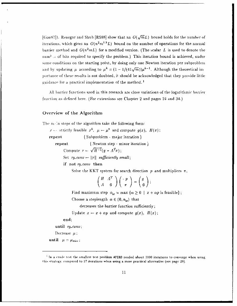
Overview of the Algorithm

The ni ln steps of the algorithm take the following form:

x - strictly feasible x° , it - it and compute g(x), 11(x);

repeat { Subproblem - major iteration }

repeat { Newton step - minor iteration }Compute r -- VH-ff (g - ATlr) ;

Set rg-conv - irJl sufficiently small;

if not rg-conv then

Solve the KKT system for search direction p and multipliers 7r,H A T

-p (

Find maximum step a, = max {a > 0 I x + ap is feasible};

Choose a steplength a E (0, aM) that

decreases the barrier function sufficiently;

Update x - x + ap and compute g(x), It(x);

end;

until rg-conv;

Decrease it;

until It = Ipn;

In a (-rude test the smallest test problem AFIRO needed about 1100 iterations to converge when using

this strategy, compared to 17 iterations when using a more practical alternative (see page 29).

11

The importance of the feasible starting point x° and its derivation are discussed in

Chapter 3.

The logical variable rg-conty indicates the convergence of the reduccA gradient 7 =

VH-1(g - AT7r). For more discussion on the issue of convergence, both for the subproblems

and for the whole problem, and on the way the /uk are chosen, see Chapter .1.

The choice of a is described in the following section.

The Steplength

For a given search direction p, the objective function reduces to a univariate function

f(a) = F(x + ap). Tile distance to the closest bound along p is a., which implies that

f(0M) = oo since the barrier function has a singularity at the boundary. The derivatives at

the endpoints of the feasible interval [O,aM] are f'(0) = gTp < 0 and f'(a,,) = x. Since

f(a) is convex, there exists a unique Q* E (O,aM) with f'(a*) = 0.

The computation of the steplength involves an iterative procedure for finding an a

close to the zero of f'. Many efficient algorithms have been developed for finding the zero

of a general univariate function (see, e.g. [Brent73]), based on iterative approximation by

a low-order polynomial. However, such methods tend to perform poorly in the presence of

singularities. In order to overcome this difficulty, special steplength algorithms have been

devised for the logarithmic barrier function (e.g. [FM69], (MW76]). These special procedures

are based on approximating f'(a) by a function with a similar type of singularity.

At each iteration an estimate aj and an interval 1j = [!j,&jJ are generated, so that

_j is the largest a encountered so far with f'(a) < 0 and Uj is the smallest a with

f'(a) > 0. The interval is initialized to I0 [0,atM]. The approximating function is of the

form

^12

where the coefficients -y and 72 are chosen such that 4(aj) = f'(aj) and 0'(0j)= f"(oj).

The zero of this function is at 04 = aM + 72171. If a4, E Ij, the new estimate is chosen

as 0j+1 = ao ; otherwise, repeated bisection is used on Ij until a midpoint aj+l is found,

such that If'(oj+i) < min{f'(p,)I,If'(5j)}.

The first a to satisfy

0 _ f'(aj) >_ Of'(0)

is chosen as the steplength a, where f E [0, 1) is a preassigned scalar. By restricting the

choice to the a with f'(a) < 0, we ensure a decrease of the objective function without

evaluating it. T .; saves the effort of computing logarithms.

12

In practice, a close approximation to the minimum of F(x + ap) can be obtained after

a small number (typically 1-3) of estimates aj . Since the minimizer is usually very close

to am , at least one variable will become very near to its bound if an accurate search is

performed. Athough this may sometimes be beneficial, the danger exists that the optimal

value of that variable could be far from its bound. Thus, performing an accurate linesearch

may temporarily degrade the speed of convergence. To guard against this, we use all upper

bound of 0.98acm instead of am, and set 0 = 0.9.

Newton's method can be shown to have quadratic convergence in a neighborhood of

the solution, provided the Hessian is not singular. In this neighborhood a step a = I is

taken. However, with the logarithmic barrier function this neighborhood is very small and

generally decreasing with yi. Given the accuracies sought in solving the subproblems, this

aspect of Newton's method is of little significance here.

13

Chapter 2

Beyond Nonnegativity

In practical problems, many variables are given bounds other than a lower bound of zero.

This more general type of linear program can be solved by the barrier inethod without

reformulation when the nonnegativity condition on x is replaced by

e < <U.

Components of x can now be free variables, fixed variables or have any combination of

upper and lower bounds, so that tj E R U {-oo} and uj E R U {00} with t < u.

More Slack Variables

The ability to define fixed variables is utilized to specify a slack variable for every constraint.

Typically in linear programming formulations an inequality constraint a~x < bi (with a'

being a row of A ) is converted to an equality constraint a~x + xn+i = bi by introducing

a slack variable x,,+i, such that x,+i >_ 0. These slack variables do not appear in the

objective function.

This concept is extended to the constraints that were originally in equality form, by

requiring that 0 < X,+i _ 0. These fixed slacks are introduced in order to make sure

that the constraint matrix A is of full row rank, regardless of possible redundancies or

degeneracy in the original formulation. The corresponding entry hn+i of the Hessian is not

defined, but we can set h-_ i = 0. (See also page 34 for an extension to these definitions.)

The General Problem

To summarize the extensions to the SLP of Chapter 1 let us update or refine some of the

definitions. The variables x are partitioned into a variable and a slack part, using the

14

notation

X ( and similarly ec= (cN , A= (A I),XM 0

where xN, CN E n", x, E R', AN E RmXn and I is the identity of dimension m. Upper-

case subscripts denote partitions of vectors or matrices, while N and M were chosen here

to reflect the dimensions n and m.

The general linear programming problem solved by our algorithm is of the form

GLP minimize cTxX

subject to Ax = b

S< X<U.

Let y = x - I and z = u - x be the distances of x from its lower and upper bounds,

respectively. The k-th logarithmic barrier subproblem is generalized to be

minimize Fk(x) = cTx _ tzk Z(ln yj + In zj)

subject to Ax = b,

and the derivatives of F(x) are given by

g = c+g", gj =-t(1/yj-1/z s )

and

H = diagh, hi = 1yj,+/Z]), j=1...,m +n.

Note that these derivatives axe well defined - even when a variable xj is not bounded

above or not bounded below. In these cases we use 1/yj = 0 for tj = -00, and 1/zj = 0

for uj = o.

Fixed Variables

When a set of related linear programs is solved, it is sometimes interesting to change the

range of a variable, and in the extreme case, fix it to a certain value. Since the iterates of the

barrier method need to be interior to the feasible region, fixed variables must be removed

from the problem. Let x be partitioned into a fixed part x F and a variable part xv, so that

corresponding partitions of the bounds satisfy IF = u, and / < u,- With the analogous

1

partition A = (A, AF), one approach is to reduce the LP problem to

Tminimize c XV

subject to Avxv - b - *tFi

_ ! _ X u",

where the objective function differs from the original by the constant c~ff..

Arithmetically equivalent is an approach that treats 1j = uj as the limiting case of

lj < u' with u --* lj. As u' - Ij we have h- 1 = h-'(u) -, 0, so that the corresponding

entry on the diagonal of the inverse of the Hessian vanishes. Partitioning the system of the

normal equations accordingly we see that

AH-'ATr = (A+ AA1 + A 0AN)r = AvII-lAr = Avlt7"gv,

which are the normal equations for the reduced problem. At each iteration, the resulting

multipliers 7r are therefore those of the reduced problem and the search direction is ]T =

( 0).

When translated into an algorithm, however, these two approaches differ in one detail.

With the reduced problem, the sparse factorization routine for the normal equations works

on the matrix A.vH:-A, whereas with the second approach, AH-lAT is factorized. Al-

though mathematically equivalent, the factorization of AvH- 1AT can be expected to be

more efficient than that of AH-AT (see Chapter 7 for the issues involved in sparse matrix

algebra). However, the formulation that treats fixed variables as a limiting case, is inter-

esting in that it offers the flexibility to fix (or free) variables dynamically for algorithmic

reasons. This technique was used in [GMSTW86] but was not investigated further in this

research.

(To preserve the full rank of A, fixed slack variables are not removed; see page 34. See

the footnote on the bottom of page 26 for a discussion of multipliers for fixed variables.)

Free Variables: a Special Case

When j =-o and uj = +oo we call xj a free variable. The corresponding entry on

the diagonal of the Hessian is hj = 'U(1/(xj - l)2 + 1/(uj - xj) 2 ) = 0 and hTl does not

exist. In this case the procedure to compute the search direction has to be reexamined. Let

16

x T = (xT xT) be a partition of x into its free and bounded parts and let A, p, c, g and

H be partitioned accordingly. The KKT system is of the form

Hb 0 Ab -Pb (b

Ab Af 0 0 2Let D be a diagonal matrix such that D 2 = Hb 1 and let r = -D-lpb. The system

above may be rewritten as(1 0DA D g,0 0 A - = (c )

AbD Af 0 r 0

As in the general least-squares formulation of page 9, the vector 7r in this equation is the

minimizer of the constrained least-squares problem

minimize JJD(gb - ATr)II2

subject to Af 7r = c1 .

Let 4' denote multipliers associated with the equality constraints Afr = cf. The

gradient of the Lagrangian of the constrained least-squares problem is of the form

L'(r,k) = AbH'ATr - AbHblgb- mf

(The factor 2 was dropped here.) With B = (AbHbAT) - 1 the solution is 7r = BAbHbIgb+

BA 1 47. Since ir has to satisfy Af r = cf , the multipliers 40 are

= (A fBA)-(cf - ABAbH-gb).

Consequently 7r is the solution of the system

AbHb'Tr = AbHb1'gb + A 1 (A BAf)-(c 1 - ABAbI'g 6 ).

Note that this formula reduces to the normal equations AbHb 1ATr = AbHblgb in the case

where all variables are bounded. Vanderbei [Van89] arrives at the same result for the affine-

scaling algorithm by treating free variables as the limiting case of -uj _< xj < uj with

Uj - 00.

This approach has computational disadvantages. The matrix ATBA 1 and its factors

must be treated as dense, even for a sparse Af . This would be inefficient for anything

17

but a small number of free columns. Also, because free variables are generally basic in the

solution, AbH-A 7' is more likely to be singular or ill-conditioned than AH- 1 A1 . 2

Instead of solving the constrained least-squares problem exactly, the following uncon-

strained penalty function (see, e.g. [VLo85]) is minimized to avoid these disadvantages:

minimize ID(gb - A67r)112 + p lf - Af r12,I

where p is a positive scalar. Denoting the solution of the approximate problem by 7r(p),

it can be shown that r(p) -, 7r as p -, o.

Solving this unconstrained problem is equivalent to solving a KKT system if) which

Hf = 0 is approximated by Iff = 1/p 1. Since gf = c1 , this corresponds to approximating

the infinite bounds of xf by two equidistant bounds If = xf - V2%,tp 1 and uf = xf +

V2V 1. These bounds are reset at every iteration and they are artificial, not only in the

sense that they are not part of the original problem, but also that they are not used when

determining the maximum feasible step along the search direction. The equivalence with

the approximated least-squares problem ensures the convergence of this approach.

Observe that Pf = -p(cf - A r(p)), where we can assume that the estimate of the

Lagrange multiplier 7r is nearly constant in p for large p. Since the maximum stepsize a

with x + op feasible is independent of the size of pf the change in the free variables IIopjfis increasing in p. A small value of p can therefore impede rapid convergence, especially

during early iterations or for unscaled problems. Conversely, a large value increases the

ill-conditioning of the problem (see page 34).

A similar problem exists for dense colums of A. They are taken out of the (main) Cholesky factorizationas suggested here for the columns of A1 . The issue of efficiency is different for dense columns, since agreat amount of computational work is saved by doing so (see Chapter 8). This suggests that solving theconstrained least-squares problem exactly bears some promise in the case where columns in A1 are dense.In particular this is true for the artificial column (see [Van89] and page 22).

18

Chapter 3

Getting Started

The algorithm as stated requires a strictly feasible (or interior) initial point. In general,

such a point can not be trivially determined.

One way to find a point that is feasible, though not necessarily interior, is to solve

an augmented linear program (ALP). The LP is augmented in the sense that an artificial

variable xa and a corresponding column of the constraint matrix is added, making any

starting point x0 with 1 < x0 < u feasible. Let ainf = b-Ax0 be the vector of infeasibilities

and let a = JIaifJ-'ainf be the normalized version of this vector; then we solve

ALP minimize xa + WcTXX,Xa

subject to Ax + axa = b

l<x<u

Xa > 0,

where w is a nonnegative weight. The artificial variable Xa E R is initialized to xa =

Ilai11 > 0, so that (x0, x° ) is feasible for ALP.

Depending on whether w is positive or zero, the solution of ALP is an optimal or just a

feasible point for the original LP. Although this approach seems straightforward, there are

difficulties, some in general and some specific to an interior-point method. In this chapter

we shall explore: (1) the implications of the choice of w; (2) better bounds for x,,; and

(3) what comprises a good starting point x° .

The Meaning of the Weight w

For w = 0 this scheme has two phases. In Phase I, the feasibility phase, we solve ALP and

obtain a feasible point for the original LP. This is taken to be the starting point for Phase II,

19

the optirnality phase, which solves the original LP for an optimal solution. The case where

no solution with xa = 0 can be found during Phase I, indicates an empty feasible region.

When w > 0, we say that ALP has a composite objective function. This approach can

be seen as a variant with overlapping feasibility and optimality phases. More cases have to

be considered for this variant and their interpretation has some ambiguity. If the algorithm

successfully terminates and x = 0, the solution vector x is not only feasible but also

optimal to the original LP. If the objective function is unbounded below, but xa = 0 for all

points on the unbounded feasible direction, the original problem is unbounded. However if

there exists a solution or a feasible direction, respectively, with x" > 0, either the feasible

region is empty or w was chosen to be too large. For every linear program there exists a

value L' so that any augmented problem with 0 < w < w' has the same solution as the

original problem. Unfortunately the determination of w' is not easy, since it would require

the solution of a nonlinear program of the same size as the original LP.

Let us examine the two-phase scheme (w = 0 ) in connection with the barrier method.

Under certain regularity conditions, the solution found by the barrier method in Phase I is

not only feasible but also interior for the LP solved in Phase II. For simplicity, consider the

linear program

minimize cTx subject to Ax = b, x > 0,X

and assume that its interior {x > 0 Ax = b} is non-empty and bounded. When the ALP

minimize xa subject to Ax + axa = b, x > 0, x, > 0

is solved by the logarithmic barrier method, the subproblems are of the form

minimize xa - p(lnx, + E-lnxj) subject to Ax + ax, = b.X'Xa

Let (x*(y), x*(p)) be the solution of one barrier subproblem. The strict convexity of the

objective function implies that x*() is also the unique optimal point of the problem

minimize -p 1 In xj subject to Ax = b - ax*(Ii),

which is formed by fixing the artificial variable at its optimal value. The limit of this

sequence of problems as p - 0 is

minimize - in xj subject to Ax = b,

20

since x*() -- 0. The objective function of this last problem is only finite for x > 0.

The solution x*(0) therefore lies in the interior of the feasible region, or could even be

defined as its center. Consequently x*(0) is a feasible interior point for the original LP.

The argument carries over for the case with upper and lower bounds. The assumption of

a bounded feasible region can be dropped when the modified barrier function of page 24 is

used.

Thus the two-phase method ( w = 0 ) would be the method of choice if it were not for the

fact that it has clear performance disadvantages compared to using the composite objective

function. Generally speaking, information about the problem gathered in Phase I is lost

when Phase II has a totally different objective function. More specifically, an approximate

solution found by the barrier method for a problem with little or no interior, will have

variables close to their bounds. This may be a bad starting point for the barrier method,

especially if the close bounds are not active at the optimal solution of Phase II. It is therefore

advantageous to have the solution of the feasibility phase coincide with that of the optimality

phase.

Experiments show that the time for overall convergence improves with increasing w in

aimost all cases. This implies that a good w would be one close to w'. A practical approach

is to set w initially to some a priori value that has performed reliably for a good range

of problems in the past, and reduce it when no satisfactory reduction of xa is achieved

during the solution of one subproblem, say. Our tests showed satisfactory results with

w E [0.0001, 1.0] for a normalized objective function, Ilcil = 1. The reduction requirement

we impose is xk <3X-1 with fi E [0.5,0.9].

Bounds on the Artificial Variable

Since we use an artificial column that is normalized, x, is the norm of infeasibilities at

every iteration. The nonnegativity constraint x, > 0 reflects this nature of the artificial

variable. However, using it as such in a barrier algorithm would make it impossible to find

a feasible point in a finite time, since variables are barred from attaining their bounds.

Consequently, we relax this bound to some sufficiently negative value, while ensuring that

xa never actually becomes negative.

Specifically, if a search direction p and a steplength a are chosen so that xa + apa < 0,

then a is reduced to a = -x/pa . At this point the artificial column is removed from the

problem and Phase 11 begins.

21

Note that this technical detail removes the structural difference between the cases with

or without a positive weight w, since it introduces a true optimality phase to the case with

w > 0. This optimality phase will usually be short for a big w, but there is still some speed

advantage from the fact that one totally dense column, the artificial column a, is removed

from the problem (see Chapter 8).

In order to remove the artificial column, an optimality phase is introduced even for

problems that have no interior. For these problems, x, approaches zero in the limit.

Phase I1 is selected as soon as the infeasibility falls below some threshold value, i.e., x" <

EeaslxIl, where cfeas is the accuracy to which we want to see the constraints Ax = b

satisfied. This tolerance cannot be smaller than the precision that can be attained when

solving the (often ill-conditioned) systems towards the end. We chose Cfeas = 10 - 6 or 10- 8

as a generally satisfactory standard.

Let us return to the question of formulating suitable bounds for xa. Although a negative

bound would never be active, the associated barrier term might still impede the convergence

of x, . Alternatively, we could impose an upper bound on x. This bound would be reset

at the beginning of each subproblem to a value slightly larger than the present value of xa

so as to encourage some progress towards feasibility.

Such reasoning ignores a peculiarity of the logarithmic barrier function, namely that,

given an a fixed by the bounds of other variables, the change in xa will increase with its

distance from a bound. If we assume for illustration purposes that the constraint matrix

A is empty, then the Newton search direction can be readily computed as p = -H-g.

Since x, cannot be defined as the norm of infeasibilities under these conditions, let x' be

any variable with ca = 1. If we impose an upper bound ua, the element of p associated

with La s pa -z/- Zwith Za = Ua - x, , or if we impose a lower bound , it is

Pa = -Y //. + Ya with Ya = Xa - la. This indicates that the change in xa depends moreon the distance to the bound than on whether it is an upper or lower bound, and that a

close bound will yield a very small change.

Naturally things look different with equality constraints, but the tendency shown here

is similar to the behavior of the algorithm observed in practice. Specifically, a lower bound

la = -1 (with ua = ) gives almost as good results as a dynamic upper bound uk = 2zk-1

(with 1a = -oo ), while both show much faster convergence to a feasible point than an upper

bound u=Z '+l1 (with 1 = -oo).

In summary, the artificial variable xa is best treated as a free variable (see page 16).

We conclude this section with one more consideration of a numerical nature. It is not

uncommon, especially with unscaled problems, to start with a point x0 that has large

22

infeasibilities, so that xa ffeas/c.M (E, = machine precision ). In these cases the roundingerror in x a makes later comparisons of xa with cfe meaningless. Additionally, errors

are accumulated in x because of ill-conditiong in the systems that determine the sequence

of search directions p. To guard against the accumulation of excessive error, the artificial

column a and x, are recomputed at the beginning of every subproblem.

Convergence is ensured by monitoring the reduction of the norm of infeasibilities Xa.

If the reduction during one subproblem falls below a satisfactory value, the weight w is

adjusted downward.

Where to start

As with most iterative methods, the choice of the starting point for the barrier function

method will have a great impact on the performance. What is special here is that any

knowledge of an approximate solution does not necessarily improve efficiency. For example,

starting off with a solution that was derived from the basis of a related LP, which is typically

clone with the simplex method, is usually undesirable. At such a starting point, several

variables are very close to their bounds. If the new optimum is not near those bounds, this

choice of a starting point results in slow convergence and possible ill-conditioning of the

normal equations.

Experience shows that subproblem k converges most rapidly when started with the

solution of subproblem k- 1. The sequence of solutions x*(k) lies on the barrier trajectory.

In order to start the algorithm on this trajectory, x0 should be a good guess at the solution

x*(0) of subproblem 0. This problem can be seen as a backward extrapolation of the

sequence of subproblems k = 1,2.... that are solved. One method to determine an x*(O)

is to solve the unconstrained problem

min F°(x) =wcTx + -f°(z),

which uses the objective function of subproblem 0. The constraints Ax° +ax ° = b are then

satisfied by setting x0 and a according to their definitions. The unconstrained problem

is separable and a solution, if it exists, would simply be the zeros of the elements of the

gradient of F0 .

A solution does not exist or is of little use for the simple logarithmic barrier function, e.g.

fj(xj) = -it n(xj - 1j) for lower bounded x. . For cj <_ 0 this function has no minimum

and even for c, > 0 the minimizer is given by xj = p°/(wcj), which may be large.

23

Linear Modification to the Barrier Function

A barrier function for which there exists a minimizer for every U, is one that includes a

linear term. Let v be a small, positive scalar and let

h (Xj) = u(lnyj -vyj), yj =xj -lj,

and

fj(xj) = ji(lnzj - vz,), z=uj -xj,

define the barrier terms of page 7 for the lower and the upper bounded variables, respectively.

(Note, for variables where both bounds l and u, are finite, the linear terms form a constant

VZ3 +vy, = v(u 3 - 1) and can be eliminated from the minimization. The result is the simple

function fj(xj) = p(ln yj + In zj) .)

The minimizers of this barrier function for the lower and upper bounded variables are

x1 = Ij + p/(pv + wc 3) and xj = uj - pl(,u- we). When we choose v such that

110 v > wIlcJI, we can disregard the linear part wcTx of the objective function. The elements

of our starting point close to the trajectory are therefore

o 1 + l/L', o =u,-1/v orXO = J+ / x0 = U- 11 r x. = (u, + lj)/2,

for the three kinds of bounded variables, respectively. Note that this approximation of the

minimum of F°(x) can be given even without knowing ji0 exactly. This is an advantage

when us0 is chosen, for example, as a function of x,.

The trajectory z*(s) of this modified barrier function differs significantly from the

trajectory of the simple logarithmic barrier function in that it is bounded. In particular,

the starting point z ° satisfies

x0 = lim x*(,1).

The consequence is that there is no danger of choosing it' too big and thereby driving the

iterates away from the solution.

Starting from the point x° as defined above, the algorithm achieves fast convergence for

the first few subproblems for a wide range of linear programs. The parameters v used were

in the range [10 -5 , 10-11. Larger values tend to give better results for scaled problems, but

are less reliable for unsealed problems.

There is some degree of freedom in choosing x° , since the objective function F(x) is

relatively insensitive to changes in x in a neighborhood of its minimizer. Additional time

savings were obtained when each xO was chosen in a neighborhood of the value above so

as to reduce the infeasibilities in A

24

Bounding the Optimal Region

It should be noted that, apart from helping to find a good starting point, the linear modifi-

cation of a barrier objective function is essential for solving a rare class of problems. These

are problems where the set of optimal points is unbounded.

Let z* be a solution of an LP that lies at a vertex, and let d be a feasible direction with

Ad = 0 and I < x* + ad < u for all a > 0. Since x* is optimal we know that cTd > 0.

If there exists a d such that cTd = 0, the barrier function subproblem does not converge

since the barrier function is strictly decreasing in a in that direction, i.e., IIx*(,U)ll --, I .

The linear modification ensures convergence to a finite minimum in that case.

25

Chapter 4

Where to Stop

Several references have been made so far to the solutions x*(k) of the subproblems and the

solution x* of the original linear program. Since both major iterations (subproblems) and

minor iterations (Newton steps) converge in the limit, we must define the point at which

we accept the current iterate as the solution.

A number of properties of an iterate x indicate its closeness to a solution. We shall

review these properties in this chapter, first for the general LP and later for the barrier

subproblems. Later we shall examine the relationship between convergence criteria and the

barrier parameters p".

Complementarity

As before, let y = x - 1 and z = u - x be the distances of x from its bounds. The

Lagrangian of the GLP of page 15 is

L(x, 7r,, 7iAx- ) )i -cT z

where irL are the multipliers for the equality constraints Ax = b and 771, 71u are those for

the lower and upper bounds. 3

3 There is some interest in computing the multipliers ilF for fixed variables z., where tF = u, (seepage 15 for notation used here). These can be calculated from the optimality conditions as 7,. = c - A 'Land correspond to the multipliers of the equality constraints Ix, = 1, had they been used to define fixedvariables instead of t 4 xF !5 up. To see that, let A be the augmented constraint matrix containing theseequality constraints, and observe

These multipliers are independent of whether the fixed variables were explicitly excluded from the problemor not.

26

Necessary conditions for optimality are

V.L TC - ArL - (77, - 7) = 0,

together with the nonnegativity and complementarity conditions

oT--

7 0, T 4'z=0.

(Throughout this discussion we assume that r7tj = 0 whenever Ij = -no and define

l j yj = 0 in this case. The equivalent holds for uj = o. )

Let rL(x), ij1 (x) and qu(x) be suitable estimators of the multipliers corresponding to

the current iterate x, so that 711(x) > 0, 71,(x) > 0 and c - AT7rL(x) - (771(x) - 7lu(x)) = 0.

If we add the condition that rltj(x) -* 0 if xj -* uj and ?7uj(x) - 0 if xj -, j, we can

estimate the sum of complementarity violations

The scalar s is an indicator of convergence, since s -* 0 for x - x * and s > 0 for every

x that is not a solution of the LP.

To derive meaningful estimators, let us recall from page 8 the other two optimality

conditions based on gradients of Lagrangians: for the barrier subproblem,

g - ATrb = 0,

and for the quadratic program solved at every (minor) iteration,

g + Hp- ATr = 0.

Since 7r - irb as x -+ x*(k) for each subproblem and 7rb --+ 7rL as / k 0 for the sequence

of subproblems, we use rL(x) = ir as the estimator of the equality-constraint multipliers.

This implies that iltj(x) = j-aT r for u1 = no, and 7).j(x) = -cj +afir for Ij = -oo. For

the case where both bounds are finite there is some degree of freedom in finding estimators.

One possible definition is

_ i zT nd Tmjx ZUj 1j(cj -aT~r) and i7.j(x) = U ( c- aj7r

These estimators are nonnegative (i.e., useful) only when the primal iterate x is sufficiently

close to the solution.

27

Duality Gap

A related idea is based on duality theory. The dual of the GLP (page 15) is of the form

maximize FD = b T rL + IT77 - uTuIrL ,771,1lu

subject to ATrL + 71 - 77u = c

771,77u > 0.

A standard result from duality is that Fo < cTx for all primal feasible and dual feasiblepoints, and that F* = cTx*, where F* is the optimal objective function value of the

DD

dual.

Using the same estimators for the dual variables as defined in the last section, an estimate

F(x) of the dual objective function can be computed. The relative difference between the

two objective functions, namely

c T x - F(x)d=DIcTxl + IF(X)l +1'

is another indicator of convergence, since d - 0 as x -- x* and d > 0 for every x that

is not a solution of the LP.

Termination of a Subproblem

The solution x*(k) of subproblem k is not interesting as such, except as the starting point

tor the subproblem k + 1. There is little need to seek a highly accurate approximation of

z*(k), since a point near the barrier trajectory should be satisfactory. It is for this reason

that the quadratic convergence of Newton's method in a small neighborhood of the solution

is of little significance.

Three vectors tend to zero in Newton's method as x x*(k), namely the search

direction p, the estimate of the gradient of the Lagrangian gL = g - ATr, and the reduced

gradient r = vrff-gL, which is the optimal residual of the least-squares problem on page 9.

All are diagonal scalings of each other, since gL = V/H-r = Hp (see page 8).

Each of these three quantities could serve as an indicator for the degree of convergence

achieved so far. During testing it was observed that Jlrli was the most consistent and

reliable measure of convergence.

28

Convergence and the Barrier Parameter

The accuracy required for a given subproblem is a function of the barrier parameter k.

Barrier subproblems with small values of u benefit more from a starting point close to the

trajectory. Only the last subproblem need be solved to the accuracy required in x*

The algorithm that controls the convergence of the subproblems is of the following form.

For subproblem k, a target level fk for the norm of the reduced gradient is computed as

a fraction of the final norm 1jrk-111 from the previous subproblem, i.e., fk = 0rJI1rk-1I. As

soon as lirli < r', a new subproblem is started with lk+i = 0,zk and a new target level

ik+1 is determined. The reduction factors 0, and 0S, must lie in the interval (0, 1) to

be meaningful. In the final subproblem, where yk = Unin, the level is set to a predefined

minimum rrin.

In contrast to a test on lIrJl, the convergence criter;a based on the complementarity

violation s or the duality gap d cannot be cmployed during early subproblems. At the

beginning, the estimates of the dual variables are inaccurate or not dual feasible, and

d ;. 1 as long as the objoctive function of the primal and the dual problem have different

signs. These criteria can be used to supplement a criterion based on JJril during the

last subproblem. In our implementation, the reduced gradient is the only indicator of

convergence used.

The values of the reduction factors determine the number of the subproblems and the

time it takes to solve each. The values used in the tests were 0, = 0.1 and Or = 0.1.

The behavior of the algorithm is surprisingly independent of the starting value /'. Values

tested were j 1 E (10 - 4 , 1) and Pnmin -- 106, both multiplied by cTx/n.

29

Part II Computing the Search Direction

Chapter 5

The Toolkit

In Part II we shall explore different aspects of solving the KKT-system

H AT)( ) ()

for the current estimate 7r of the multipliers and a search direction p.

Premultiplying the first part -Hp+ATr = g by AH- 1 , we derive the normal equations

AH-'AT7 r = AH-'g.

The matrix AH-1AT is symmetric and positive definite. Since A is of the form A =

(AN I), let H = diag(H,,, HM,) be partitioned accordingly. The nonzero structure of the

product AH-1AT = ANH;AT +N H,; can be seen to be that of ANAT. The efficiency of

recent methods for forming the triangular Cholesky factors AH-'AT = LLT (see [GL81,87])

has given the normal equations a prominent role in the implementation of interior-point

algorithms.

Before going into the details and potential hazards of this approach in the following

chapters, we review some alternatives and their characteristics.

The Least-Squares Problem

In Chapter 1 we mentioned that the term "normal equations" is derived from the weighted

least-squares problem (page 9)

minimize IIDg - DAT1rII ,

which is equivalent to the KKT-system with D2 = H - '.

However, there are other ways of solving large sparse least-squares problems. Three of

these methods, two direct and one iterative, are described below.

30

The QR Factorization

Let C = DAT be the matrix associated with the least-squares problem. There exist an

orthonormal matrix Q and a factor R such that

C =QR =(QI Q 2 ) (R0

where R1 is square and upper triangular. Since the Euclidean length of a vector is invariant

under an orthogonal transformation we can rewrite the norm of the least-squares problem

as

jbg - = 1QTD9 - QTCT 2 = IIQTDg - RJ II2 = I1QiDg - R1irII 2 + IIQ2Dg1 2 ,

so that the optimal 7r is the result of the backward substitution R1 7r = Q1 Dg.

Strong error bounds can be derived for the QR factorization in finite-precision arithmetic

(see [GVL83]), which makes it more desirable than the Cholesky factorization in terms of

numerical stability.

The disadvantage of the QR factorization is its computational cost. The number of op-

erations involved in a sparse QR factorization is considerably larger than that of a Cholesky

factorization of AH-A T especially when A is very rectangular. (See [GN84] and [GLN88]

for implementations of sparse QR. The matrix Q need not be stored in our case, but stands

for a series of orthogonal transformations applied at the same time to C and Dg. )

Given what we know about the QR factorization today, we do not expect interior-point

methods based on this factorization to be competitive.

The Semi-Normal Equations

Note that the Cholesky factors of AH-AT are related to the QR factors of C. We have

LLT = AH-1AT = CTC = RTQTQR = RTR = RTRI.

Thus L can be computed by performing the QR factorization and setting L = RT . The

method of semi-normal equations consists of forming L this way and solving for 7r with

the normal equations LLTr = AH-lg.

The numerical properties of this method are analyzed in [Bj87a]. Although the tri-

angular factor is of better "numerical quality", the error in 7r is shown to be about the

same as that obtained from Cholesky factorization. The only improvement is in the bound

on the condition number of C to achieve a numerically non-singular L. The concern of

computational inefficiency with the QR factorization applies as before.

31

The Conjugate-Gradient Method

One algorithm for solving the least-squares problem that is not based on a matrix factor-

ization but on a series of matrix-vector products, is the conjugate-gradient (CG) method.

Starting at an initial point 7ro, the method proceeds by taking steps along a sequence of

search directions Uk . With initial values r0 = Dg for the residual, ul = so = CTDg and

70 = ls01l2, each iteration includes the following steps for k = 1,2,..

qk = Cuk

alk = 'k-1/IiqkII 2

k = lrk 1 + OkU k

rk = rk_ 1 - kqk

Sk = CTrk

1k = IIskIlI

A+ = Ykfk-

Uk+1 = Sk + OkUk•

Certain orthogonality relations can be shown (see e.g. [HS52]); in particular, sTu3 0,

sTs1 =0 and uJCTCu, =0 for j= 1,...,k-1.

In theory, this procedure can be considered a direct method since it converges in a

number of iterations that is equal to the number of distinct singular values of C. In practice,

rounding errors cause the algorithm to behave like an iterative method, and termination

may occur whenever 1ski1 is sufficiently small. It is still observed to perform best on

problems where the singular values of C are clustered in groups.

Variants of the conjugate-gradient method have been used successfully in implementa-

tions of interior-point methods, see [GMSTW86], [KR88]. The version used in [GMSTW86]

is LSQR by Paige and Saunders [PS82] which is very well suited for solving least-squares

problems. Other CG methods solve a system of the form Bx = y and can be applied to

the normal Pquiations. Some vector operations may be saved that way, but it has much less

desirable numerical properties.

The matrix C may be transformed into a matrix with clustered singular values by using

a preconditioner. Let R be the nonsingular Cholesky factor of a matrix that approximates

CTC. The problem

minimize IDg - CR -1 zll2

32

can usually be solved using CG in fewer iterations. The original solution is recovered by

solving Rr = z.

At each CG iteration the main work is in forming products of the form CR-lu and

(CR-)Tv. The savings obtained by factorizing an approximation of CTC compared to

factorizing the exact matrix, have to be large enough to offset the cost of the iterations.

The success of this approach lies entirely in the ability to devise a sparse preconditioner R

such that RTR has eigenvalues close to those of CTC.

The Nullspace Method

An alternative approach to solving for 7r first is one based on the observation that p lies

in the nullspace of A. Let Z be a matrix whose columns span the nullspace of A, so that

AZ = 0 and for every p with Ap = 0 there exists a linear combination Pz of the columns

of Z such that p = Zp, . The first part

-Hp + ATir = g

of the KKT-system is premultiplied by ZT to give

ZTHZpZ = -Zrg.

As before, this system is symmetric and positive definite. It can be solved either directly

by forming Cholesky factors, or by applying one of the previously discussed methods to the

least-squares problem

minimize JIDg - D-'1ZP 2.PZ

For the special structure of A = (AN 1in), a matrix whose columns span the nullspace

is given by

Observe that the sparsity structure of the positive-definite system ZTH Z = HN + ATIIMANis that of A NAN. Since most linear programming problems have more dense rows than

dense columns, this matrix is likely to have more nonzero elements (and hence be harder to

factorize) than one of the form ANAT. (For more on the issue of comparing these sparsity

structures, see page 54.)

33

Chapter 6

Ill-conditioned Systems

It is common for the matrix AItIAT of the normal equations to have a high condition

number. The ill-conditioning may arise because A and/or H -1 are ill-conditioned.

The matrix AH-1AT = ANH 'AT+ H- 1 is near singular or singular when AN is ill-

conditioned and the diagonal of JI1 has some zero entries. 4 This is due to degeneracy in

the formulation of the original problem. To detect degenerate rows that are redundant is a

hard combinatorial problem. In addition, near rank-deficiency is likely to occur in problems

that are poorly scaled.

Near-singularities occur also if the number of diagonal entries in H approaching zero

is greater than n, which is a typical behavior towards the end of Phase I or Ii when many

variables are approaching their bounds.

More Slack for Fixed Slacks

The problem of a nearly rank-deficient A can be eased by introducing small bounds onthe fixed slacks -, of rows that were originally equality constraints, i.e., the constraints

0 <x<0 are replaced by -61 < x < b61 with 6>0.

When 6 > 0, all diagonal entries of II are nonzero and AH-IAT is strictly positive

definite. At the same time, the dimensionality of the feasible region is increased, possibly

creating a strictly interior region. The parameter tt of a barrier function associated with

these bounds is to be treated differently. Reducing pt, from one subproblem to the next,

does not help the convergence of the subproblems to the original problem. We would

therefore like to keep ps constant and big, say /I ; 105, in order to ensure that It > jk

for any k.

4 We continue to use 11,; as a symbol, even if it is singular and HM is not defined. This case may beviewed as the limit of shrinking bounds on the fixed slack variables.

34

Naturally, such bounds affect the precision with which the original constraints are satis-

fied at the solution. Let x,,+i be an entry in x, and 7rLi the multiplier of the corresponding

constraint at the solution. Since g = AT rL, it follows that

1 1 o -/= -I- 2+ 6 2 r 2

-- Li or x Lt+f,+i Li

Assuming that 17LI << p/, the value x*+i can be approximated by (62 rLi)/(2,uS). Since

1iIl < 10' for all but the worst scaled problems, a bound 6 = 10- 4 yields a solution that

satisfies the feasibility tolerance Efe, = 10-6.

As far as AH-1AT is concerned, introducing no bounds on the fixed slacks, i.e. setting

= 0, is equivalent to removing the corresponding columns from A. Tests with scaled

problems showed that this reduced constraint matrix was sufficiently well-conditioned in

all but a few cases. It was also observed that the performance of the algorithm on other

problems was degraded by introducing artificial bounds on fixed slack variables. In our

implementation, 6 is therefore a user-selectable parameter with a default value of zero. It

has to be set to a positive value for problems where difficulties caused by the rank of A are

encountered, and it can be reset to a smaller value when the resulting residual JjAx - b~l is

deemed too large.

A Theoretical Bound

Concerning the difficulties introduced by an ill-conditioned H- 1, Dikin [Dik67] and Stewart

[Stew87] show for a full-rank A that

sup II(AH-lAT)- 1 AH- 11 < oo.HED+

The set V+ is the space of diagonal matrices with positive diagonal elements. Since rr =

(AH-1AT)- 1 AH-lg and H E D+ by its definition, we should expect from this result thatthe numerical error in 7r is also bounded. However, short of using a QR factorization, we

do not know how to form the matrix (AH-lAT)- 1 AH- 1 without forming (AH-1AT) -

first (i.e. forming and factorizing AH-1AT). Since Ij(AH-AT)- 11 cannot be bounded on

D+, the error has already been introduced at this point. The following are measures to

improve the accuracy of ir and to reduce the condition number of AH-AT.

35

Updating r

When computing the r of one (minor) iteration, a fairly good estimate is already available

in the form of the multiplier estimate f" of the previous iteration. This is especially true

towards the end of a barrier subproblem when 7r -* 7r* (i). In order to avoid rounding

errors and to reduce the impact of catastrophic cancellations, the change q - -r is

computed rather than 7r itself.

Therefore, the system solved to determine a new search direction p is of the form

AH-1ATq = AH-'gL

p = -H-1gL,

with L = g - ATir and gL = #. - ATq = g - ATir. The vector is denoted by gL because it

converges to the gradient of the Lagrangian (page 8).

Diagonal Correction

The computed search direction p must satisfy two conditio:.s. First, it must be close to the

null space of A, which means that [lAp[I/lip{ I < c for some suitable f > 0. Second, it must

be a descent direction for the barrier objective function, i.e., gTp < 0. These conditions are

satisfied as long as q is an exact solution for the system above, since

Ap = -AH-1 # + AH-ATq = 0

andTT=_LHIL+7A < 0gp (g + ATr)Tp

for any feasible, non-optimal point (x, r). Observe that gTp = _gLTH-lg L is less than zero

if Ap = 0, independently of the accuracy in 7r. We can therefore focus on Ap as the error

term in question.

In order to model the error introduced into q, assume q to be the exact solution of the

system

(AH-AT+ E)q = AH-1iL,

where E is an error matrix. The error term is then

Ap = Eq.

36

The error matrix E is small except for matrices AI-I'AT that are very ill-conditioned.

In this small neighborhood of singularity there also exists some danger that the Cholesky

factorization might break down because of diagonal elements that become extremely small

or negative due to rounding error. One way to guard against a break-down or the large E

associated with very ill-conditioned matrices is to add a correction matrix F to AH-IAT

that improves its condition number. Let E(F) be the error matrix associated with the

system AH-IAT+ F. Then F should be chosen so that [IF + E(F)II is minimized, which

means, F should be the smallest correction that brings AH-AT+ F out of the neighbor-

hood of singularity.

A good and simple choice for F is a diagonal matrix that reduces the quotient l,,x/lin

of the largest and smallest diagonal elements of the factor L. This heuristic is based on

the fact that the condition number of AH-AT is bounded below by (.maxllmin) 2 .

The correction matrix F may be formed during the factorization, by using all zero

entries except for those indices i where the diagonal of L is below some threshold value,

i.e.,

Fi = (max{/ Imax - Lii, 01)2,

for some 0 < Iy K< 1. This definition is used in our implementation. The correction Fij

is computed at the point where Lii is determined during the factorization. Such a choice

for F has the advantage that F is zero for well-conditioned systems and relatively small

otherwise, and that a bound lmax/Imin <. 1/-y is enforced. Nevertheless, examples of near-

singular AH-IAT can be constructed, where the correction can grow to IIFI = 2mc, (, =

machine precision). Since the exact 1max is not known until the factorization is complete, we

use an estimate for determining Fii . The estimate is lmax(i) = max{0.1 1,m", Ljj for j =

,... i - 1}, where "max is the maximum of the previous iteration. In tests we used a

threshold factor -/ = 0.1V/CM.

Modified Hessian

We would expect to be able to improve on the error term by taking the correction F to

the diagonal of AI-LIAT into account when subsequently computing p. Since

AH-AT + F = -ANH AT + H,7 + F,

where both il;I and F are diagonal matrices, this change is simple. Instead of using IV'

when computing the search direction, we could use

t1= t-1+ (ON 0 O)7

37

and get the error term Ap = E(F)q. This error can easily be made suitably small by

choosing F large enough.

However there are other factors that determine the quality of a search direction. For

a convex function, using the exact Iessian when computing p gives Newton's method

quadratic convergence in the neighborhood of the solution. Although this quadratic con-

vergence is rarely seen in practice with such a non-quadratic function as the logarithmic

barrier term, making the change to the Hessian suggested above reduces the rate of conver-

gence considerably. Numerical tests have shown that corrections that are small enough to

give an acceptable rate of convergence were not always able to reduce the condition number

of AII-1AT sufficiently.

Iterative Refinement

For a general square matrix B, the error in a solution x of the system Bx = y can

often be reduced by performing iterative refinement. It involves repeatedly computing the

residual r = y - Bx and solving Bz = r to give a better solution x' = x + z. No additional

accuracy can be expected with iterative refinement when the first x was found by Gaussian

elimination (of a reasonably well-scaled matrix) and r was computed to the same precision

as x (see e.g. [GVL83]).

In our case we do not have the option of calculating an r = AH-#, - AH-ATq = Ap

to more than the precision generally used for all variables. Also, the Cholesky factorization

of AH-1A r is equivalent to Gaussian elimination.

However, if a diagonal correction F is introduced during factorization, the accuracy of

q can be improved when residuals are computed from AH-1AT. The iterative refinement

is implemented in the following form:

gL --- gL

repeat

LLTq Ap

update r .- r + q, g, - gL- A Tq, p p + H-'Aq

until IlApil acceptable.

Convergence can be shown (see e.g. [Bj87b]) if

p(I - (LLT)-IAH-IAT) < 1,

38

where p(.) denotes the spectral radius. This translates into a bound on tho size of F.

Convergence criteria for the residual rA = Ap are twofold. First, a static upper bound

on acceptable values for Jjr.j /I]AH-gLI is given. We choose this conservatively to be E/.

Second, little progress in reducing lirAjl is taken as a sign that the remaining residual is

inevitable. Average cases show a reduction of IIrAjI by a factor of about 10-2 for every

iteration of the refinement.

Applying iterative refinement to the normal equations is equivalent to refining the KKT-

svste In

,4 0 )(q

and using normal equations at each step. The residual of this system is

Ap Ap

since -Hp1 = -g, = gL - ATq independently of the accuracy of q. Forming the normal

equations for the KKT-system with r' as the right-hand side yields a right-hand side

rA = Ap for the normal equations, as before.

39

Chapter 7

Inside the Factorization

The first step towards the computation of the Newton search direction is the solution of the

normal equations

AH-1ATq = AH- g,.

This system is solved by computing the Cholesky factorization,

AH-IAT = LLT

and solving the triangular systems

Ly = AH- 1 g, and LTq = y.

The time for computing the search direction dominates the time per iteration - typically

80%-90% of the total for a medium-size problem, but it can be as high as 99% for the

largest problems. For the linear programs of interest, the matrices A and, to a lesser

degree, AH-1AT and L are sparse, meaning that almost all their elements are zero. An

efficient way to form and factorize these large sparse matrices is therefore crucial to this

implementation of the barrier method.

Other interior-point methods share this need, since they also solve a symmetric positive-

definite systems of the form ADA T , with D diagonal. (See Adler et al. [AKRV87] for

programming techniques, or Monma and Morton [MM87]). Thus many of the following

observations are equally relevant to these methods.

In our implementation the Cholesky factorizations is performed by the subroutines of

SPARSPAK-A by Chu, George, Liu and Ng [CGLN84], with minor modifications.

The actual numerical factorization is preceded by an Analyze Phase, in which the

nonzero patterns of the involved matrices are analyzed and the necessary data structures

are established. These procedures are covered in Chapter 9. For the scope of this chapter

we shall ignore the problem of dense columns in A. Extensions to algorithms and data

structures taking that issue into account will be described in Chapter 8.

40

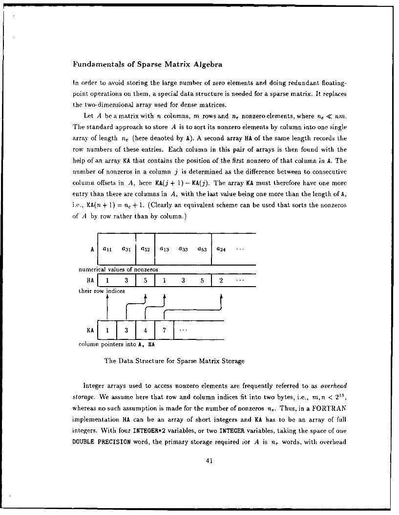
Fundamentals of Sparse Matrix Algebra

In order to avoid storing the large number of zero elements and doing redundant floating-

point operations on them, a special data structure is needed for a sparse matrix. It replaces

the two-dimensional array used for dense matrices.

Let A be a matrix with n columns, m rows and ne nonzero elements, where ne < nm.

The standard approach to store A is to sort its nonzero elements by column into one single

array of length n, (here denoted by A). A second array HA of the same length records the

row numbers of these entries. Each column in this pair of arrays is then found with the

help of an array KA that contains the position of the first nonzero of that column in A. The

number of nonzeros in a column j is determined as the difference between to consecutive

column offsets in A, here KA(j + 1) - KA(j). The array KA must therefore have one more

entry than there are columns in A, with the last value being one more than the length of A,i.e., KA(n + 1) = n, + 1. (Clearly an equivalent scheme can be used that sorts the nonzeros

of A by row rather than by column.)

IA all a3, I a52 a13 a 33 a53 a24 ..

numerical values of nonzeros

HA 11 3 5 11 3 5T 2 .

their row indices

KA I11 3 4] 7 -

column pointers into A, HA

The Data Structure for Sparse Matrix Storage

Integer arrays used to access nonzero elements are frequently referred to as overhead

storage. We assume here that row and column indices fit into two bytes, i.e., m,n < 215,

whereas no such assumption is made for the number of nonzeros n,. Thus, in a FORTRAN

implementation HA can be an array of short integers and KA has to be an array of full

integers. With four INTEGER*2 variables, or two INTEGER variables, taking the space of one

DOUBLE PRECISION word, the primary storage required ior A is ne words, with overhead

41

storage of -n, + -i words.

For the rest of this chapter a sparse vector or a sparse matrix will be a vector or matrix

whose nonzero elements are stored in the described way. A dense vector or a dense matrix

denote a vector or matrix stored in the usual way, regardless of the actual proportion of

zero to nonzero elements in them. Assignments between a sparse vector and a dense vector

will refer to the copying of nonzero elements of the dense vector to or from a sparse data

structure. Row i of a matrix A will be denoted by ai , and column j by a .

Several observations are in order. First, a given element aij of a sparse matrix cannot

be accessed without doing a search along its column j for an entry in HA with value i.

For efficiency reasons any sorting and searching of elements should be avoided in these

computations, with the exception of the Analyze Phase. The numerical operations we

do on sparse matrices should thus be restricted to those that work sequentially on whole

columns.

The set of sparse vector operations that do not require sorting, searching or additional

workspace include scaling a sparse vector, s, = a so ; adding a multiple of a sparse vector

to a dense vector, d, = do + a s; and computing the inner product of a sparse vector with

a dense vector, /3 = dTs, or with itself, J/ = sTs. Not included in this set are operations

such as the inner product of two sparse vectors, /3 = sTs2 ; or their sum, S3 = 31 + S2, in

the case when the result is to be treated as a sparse vector.

With A stored by its sparse columns aj , the product d = Ax is computed as d =

Fxja,, whereas the product with the transpose e = A T is composed of ej = ay. Here

x, y, d and e are assumed to be dense. Observe that the elements of aj do not have to

be sorted by row index in HA for these operations. This fact gives a degree of freedom that

we will exploit during the factorization, below.

Forming AH-1AT

Let B denote an m x m matrix containing the lower-triangular half of AH-1AT,

B = tri(AH-IAT ) where bij = { 0Afor i <j

(AH-AT for i > i.

Since only half of a symmetric matrix is stored in practice, the matrix to be formed is

actually B.

42

One way to compute this scaled outer product is by computing each element bik as a

scaled inner product of rows of A,

for k = 1 ... m

for i = I ... kbik = a'H-la ,

T .

Sk

This is not easily implemented for a sparse A, because even if A is stored by rows rather

than by columns, the inner rr-duct of two sparse vectors is not an efficient operation.

Computing B by explicitly adding the column outer products B = E 1/h,, tri(aJaT)

is not possible without keeping B temporarily in a dense representation, which requires

prohibitively much memory.

One solution is a scheme that rearranges the second loop of the algorithm above and

requires a dense vector d as temporary storage. Let a define the lower part of aj, so

that 0 for I< ka(j for £>k.

The algorithm for forming AH-1AT then becomes

for k =1 ... m

d=O

for j such that akj j 0

d = d + (akj/hjj) ak

bk = d.

Here only columns of B and A are accessed. The question of finding the elements of a4k

without searching for them in the column aj will be addressed on page 45.

Factorizing AH-IAT

Since AH-AT is a symmetric positive-definite matrix, there exists a Cholesky factorization

AH-AT = LLT , where L is lower triangular. The method to compute it should have the

property that B gets overwritten by (part of) L. Of the three methods with this property

described by George and Liu [GL81], the inner-product form is used in the SPARSPAK

package:

43

for k=... mk-i

kk= bkk - Zj=1

for i=k+1 ... mk-i

lik= bik - 1j lkjlijj=i

I= (IV'ilk.

As before, the inner product of two rows is avoided by reformulating the second loop,

using l as the lower part of 1j:

for k = ... m

d= bk

for j such that lki $ 0

d = d - lkj 1Ilk ( (1 / V/' ) d.

When examining this procedure for the resulting nonzero structure of L, note that L

has a nonzero wherever B has one, but might have more. This property allows a general

B to be stored in the same sparse matrix structure as L. (This feature becomes irrelevant

for the special case of AH-1AT by the observation in the next section.)

The minor effort of computing m square roots can be saved by using the factorization

AH-1AT = LDLT instead. Here L is an unit lower triangular matrix and D is diagonal

(see [AKRV87]). Since taking this approach would add several scalings with D- 1 to the

computation of the Schur complement in Chapter 8, its advantages in our implementation

are not clear and this path was not taken.

Forming and Factorizing in one Step

The similarities between the two algorithms sketched above are striking. Both arise from

an inner-product form; both have a dense vector to accumulate multiples of lower parts of

sparse columns; ii, both cases this depends on the column element in the current row.

The outer loops of both operations have an index running over the same range, one

ending with bk = d, the other starting with d = bk. Checking that bk is not accessed

when computing any l with j < k, we see that it is not necessary to form B explicitly.

Instead we can form and factorize each column of L in one step.

44

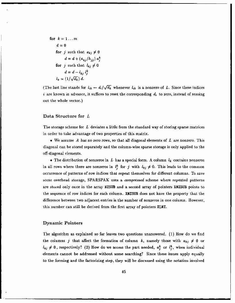
for k = 1 ... md=0

for j such that aki X 0

d = d + (ak,/hjj) a4

for j such that Iki 0 0

d = d - Iki '1j1k = 1Vk d.

(The last line stands for lik ,- di/Vd'k whenever lik is a nonzero of L. Since these indices

i are known in advance, it suffices to reset the corresponding di to zero, instead of zeroing

out the whole vector.)

Data Structure for L

The storage scheme for L deviates a little from the standard way of storing sparse matrices

in order to take advantage of two properties of this matrix.

* We assume A has no zero rows, so that all diagonal elements of L are nonzero. This

diagonal can be stored separately and the column-wise sparse storage is only applied to the

off-diagonal elements.

9 The distribution of nonzeros in L has a special form. A column 1k contains nonzeros

in all rows where there are nonzeros in 1 for j with 'kj j 0. This leads to the common

occurrence of patterns of row indices that repeat themselves for different columns. To save

some overhead storage, SPARSPAK uses a compressed scheme where repeated patterns

are stored only once in the array NZSUB and a second array of pointers XNZSUB points to

the sequence of row indices for each column. XNZSUB does not have the property that the

difference between two adjacent entries is the number of nonzeros in one column. However,

this number can still be derived from the first array of pointers XLNZ.

Dynamic Pointers

The algorithm as explained so far leaves two questions unanswered. (1) How do we find

the columns j that affect the formation of column k, namely those with aki X 0 or

lki 0, respectively? (2) How do we access the part needed, ak or 1k, when individualelements cannot be addressed without some searching? Since these issues apply equally

to the forming and the factorizing step, they will be discussed using the notation involved

45

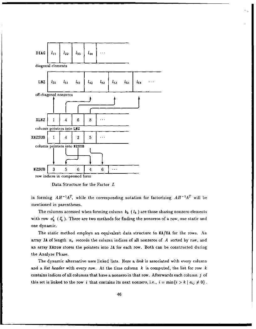
DIAG [111i 122 133 144 .

diagonal elements

LNZ 131 151 161 142 162 153 163 164

off-diagonal nonzeros

XLNZf1j 1 4__1_6__8_

column pointers into LNZ

XNZSUB 1412 5

column pointers into IZSUB

NZSUBF3 5 6 4 6

row indices in compressed form

Data Structure for the Factor L

in forming AH-AT, while the corresponding notation for factorizing AH-1AT will be

mentioned in parentheses.

The columns accessed when forming column bk (lk ) are those sharing nonzero elementswith row a' ( l ). There are two methods for finding the nonzeros of a row, one static and

one dynamic.

The static method employs an equivalent data structure to KA/HA for the rows. An

array JA of length n, records the column indices of all nonzeros of A sorted by row, and

an array KArow stores the pointers into JA for each row. Both can be constructed during

the Analyze Phase.

The dynamic alternative uses linked lists. Here a link is associated with every column

and a list header with every row. At the time column k is computed, the list for row kcontains indices of all columns that have a nonzero in that row. Afterwards each column j of

this set is linked to the row i that contains its next nonzero, i.e., i = min{i > k I aij $ 01.

46

The next nonzero in a column can be found without searching when the nonzeros of

each column are sorted by row index inside A/HA. So, unlike simple matrix operations, such

a scheme requires a special order for A. (See also 'Permutations', below.)

The ordering is also needed to answer the second question, the problem of accessing ak(l ). A second, dynamic array of pointers over all columns KA1ST (FIRST), initially set

to KA (XLNZ), is used to point to the first element of a (l ) for the next column k that

is going to use column j. Again, this array can be updated after column k is computed

simply by adding one, so that, say KA1ST(j) now points to the first element of a , where

i is the row with the next nonzero, as above. The last element of any a is the same as

the last element of aj and sits at offset KA(j + 1) - 1. This way of accessing the lower part

of the column is independent of whether the column was found by the static or dynamic

method above.

The similarity of the algorithms for forming and factorizing should imply that we choose

the same data structure for finding the right column in both cases. However, the deter-

mining dimensions are not of the same order. Additional overhead storage needed for the

alternatives are (in terms of full INTEGERs)

Forming Factorizing

static n,(A)/2 + n n(L)/2 + m

dynamic (n + m)/2 m/2 5

As we expect there to be more off-diagonal nonzeros in L than nonzeros in A, the

time savings from avoiding the maintenance of a linked list in the static method are gained

at the expense of more memory during the factorization. In our implementation we leave

intact the linked list used in SPARSPAK for L, but use the static access scheme for the

rows in A.

Permutations

The outline of the procedure to factorize AH-IAT has omitted one important aspect.

Although the number of nonzeros in AH-AT is independent of the row permutation of

A, the number of nonzeros in L is not. During the Analyze Phase, see Chapter 9, a

permutation P is sought that minimizes the fill-in of L. Thus the actual factorization is

of the form

PAHI-ATpT= LLT.

s For the factorization, both the list headers and the links can use the same array of length 171 since theoff-diagonal nonzeros of row i can only lie in columns j with j < i

47

KArov 1 1 3 1 6 7

I L

JA 1 1 3 14 1 1 3 6 2 3

column indices of nonzeros

A a3 all a52 a33 a53 a13 a24 .

their numerical values

HPA 1 1 4 12 1 2 4 6

their permuted row indices

KA1ST 1 2 3 1 5 7offset of a5 (with i = 2), dynamic

HA 13 1 15 13 5 1 2 --

their original row indices

I __________________ I_

KA I J 1 1 1column pointers into A, HA, HPA

Data Structure for A during factorization

48

By rewriting PAH-ATpT as (PA)H-1 (PA)T, we leave the factorization as it is, just

using PA instead of A. This is done without any additional work by introducing an

additional array HPA that contains the permuted row index for each nonzero. Sorting the

entries of A, HA and IIPA so that the entries in HPA are in ascending order for each column,

completes the adjustments that have to be made for the permutation. All this is done

during the Analyze Phase.

Gay [Gay88] suggests that some permuting of vectors can be saved when columns of L

are stored in the order of the corresponding row indices of A. This idea was not followed

here, since keeping L and other vectors and matrices in the permuted order is essential for

some details of the implementation of the Schur complement (see page 55).

49

Chapter 8

When Things get too Dense

The sparse constraint matrix of the linear program in Phase I can be written in the form

A = (AN a I), where a denotes the artificial column. Since a is assumed to have no

structural zeros, aaT and thus AH-1AT are dense matrices. A similar problem can also

occur in the optimality phase, i.e. when a = 0. Including all the columns of AN when

forming AH-1AT can sometimes be uneconomical at best, often making it impossible to

run a certain LP on a memory-constrained machine. The columns we would like to omit

from AH-AT will be called dense columns, although factors other than the mere number

of nonzero elements might contribute to the definition of this set, see page 52.

Schur Complement

Assume that there are nd dense columns (including a), and let Ad be the submatrix of

AN that contains them. Defining the partitions

A (A, Ad I) and H = diag(Hs, Hd, HM)

we have

AH-AT= ASH.'AT + HtM' + AdH dA ,

where A,118 7AT + HM 1 has a sparse triangular factor L.

Taking the matrix square root V = AdHd 112 of the remainder, the solution of the

normal equations AH-IATq = y can be found from the larger system

(L L T V z

(Equivalent formulations, with V = Ad or V = AdI! 1 and Hd or Hd"1 in the lower right-

hand corner, yield somewhat cleaner notation but proved to be less stable numerically.)

50

The matrix C = I + WTW, where W = L- V, is called the Schur complement of LLT.

The required solution q may be determined by solving the following sequence of equations:

Ls = y

Cz = WTs

LTq = s - Wz.

The numerical accuracy of the solution may be improved by iterative refinement, see

page 38, when nd > 0. In practice we have observed that only one additional refinement

step is worthwhile. In the rare case where the residual rA = y - AH-ATq turns out to be

already very small, this step may be skipped.

Comparison with preconditioned CG

Dense columns of A present a difficulty for all interior-point methods that factorize a matrix

of the form ADAT with D diagonal. An alternative approach is to use the Cholesky factor

of A a1 A HT,+ as a preconditioner for a conjugate-gradient method (see page 32).

The two approaches are not the only alternatives. A hybrid method is possible, where

the Schur-complement method works inside CG. The preconditioner could be improved this

way to include dense columns aj where hi - 1 is large. Or the conjugate-gradient method

can be employed to cope with corrections made to L during the factorization. Such a

hybrid method was not tested in the scope of this research.

We shall compare the Schur-complement method to a CG implementation that uses

LSQR [PS821. To have some measure of the work performed beyond the factorization, we

identify two important parts, namely the solves, LTx = b or Lx = b, and the products, Au

or AT:, for some vectors x, u. CG needs 2 solves and 2 products for start-up in addition to

2 solves and 2 products per iteration. Whereas we can treat the Schur-complement method

with two steps of iterative refinement as a direct method, LSQR is an iterative method.

Typically it was observed to take 2 iterations in the case of one dense column and some i

iterations in the case of nd > I dense columns, with nd + 1 < i < 2 nd.

To compare the work per barrier iteration with the two approaches three cases are

considered:

e nd = 0. In this case AH-IAT = LLT and the normal equations can be solved di-rectly. Neither CG nor the Schur complement need be employed, both are identical here.

51

*nd = . One solve is needed to compute 14', plus two per step of the iterative

refinement. Computing the residual costs two products. Any additional work is negligible.

This adds up to 5 solves and 2 products, which compares favorably to 6 solves and 6

products with CG. Typically the dense column here is a, which has a density of 100%.

This distinguishes it from the next case:

e nd > 1 . Again two solves are needed per step of the iterative refinement and two

products to form the residual. Computing W takes exactly nd solves, giving a total of

nd + 4 solves and 2 products. CG takes at least 2 ?td + 4 solves and 2nd + 4 products. The

additional work needed to compute the Schur complement C = I + wTw is significant

here, but so are the savings obtained by taking advantage of the sparsity in V when forming

LTW1 = V.

Comparison of Storage required

Here the case nd = 0 is not relevant, since storage always must be allocated for the

maximum need, which is during Phase I. Storage requirements for the Schur-comploment

are less in the case 7d = 1, since some work vectors needed by LSQR can be saved in an

efficient implementation.

Analytically it is unclear, however, how the methods compare in the case nd > 1.

Although W must be stored, this can be done effectively in some sparse format (page 55),

since it is typically only 25%-75% dense. Because of the great time advantage, the time-

optimal choice for the number of dense columns is bigger than with CG. This in turn reduces

the density of L considerably. Experiments with a small number of LP test problems with

dense columns, suggest that the size of L and W together for a time-optimal choice of Ad

is substantially less than the size of L alone for a choice of Ad that would be optimal with

a conjugate-gradient method.

Identifying a Dense Column

The definition used in our implementation is simple: if a column has more than a preassigned

number of nonzeros, it is handled as a dense column. This threshold number can be set

by the user. If it is not specified it defaults to a rule of thumb involving the number of

rows m. 6

6 The number used is set up to make a near-optimal choice for the four or five problems of the test set

with dense columns: 3m + 700.

52

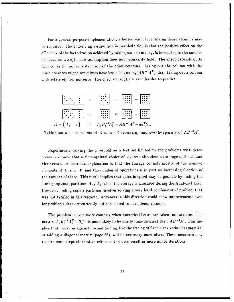
For a general-purpose implementation, a better way of identifying dense columns may

be required. The underlying assumption in our definition is that the positive effect on the

efficiency of the factorization achieved by taking out column aj , is increasing in the number

of nonzeros n.j(aj). This assumption does not necessarily hold. The effect depends quite

heavily on the nonzero structure of the other columns. Taking out the column with the

most nonzeros might sometimes have less effect on n,(AH- 1 A T ) than taking out a column

with relatively few nonzeros. The effect on nz(L) is even harder to predict.

A = (AI a) = AIHi'AT= AH-'A T -aa T/ha

Taking out a dense column of A does not necessarily improve the sparsity of AH-'A7 T

Experiments varying the threshold on a test set limited to the problems with dense

columns showed that a time-optimal choice of Ad was also close to storage-optimal kand

vice-versa). A heuristic explanation is that the storage consists mostly of the nonzero

elements of L and 11' and the number of operations is in part an increasing function of

the number of these. This result implies that gains in speed may be possible by finding the

storage-optimal partition A, / Ad when the storage is allocated during the Analyze Phase.

However, finding such a partition involves solving a very hard combinatorial problem that

was not tackled in this research. Advances in this direction could show improvements even

for problems that are currently not considered to have dense columns.

The problem is even more complex when numerical issues are taken into account. The

matrix A, H1AT + H,71 is more likely to be nearly rank-deficient than AH-IAT. This im-

plies that measures against ill-conditioning, like the freeing of fixed slack variables (page 34)

or adding a diagonal matrix (page 36), will be necessary more often. These measures may

require more steps of iterative refinement or even result in more minor iterations.

53

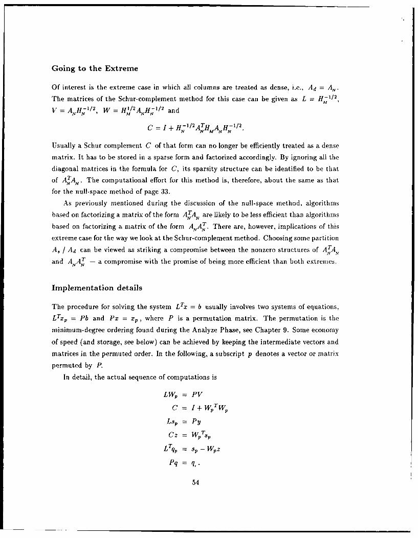
Going to the Extreme

Of interest is the extreme case in which all columns are treated as dense, i.e., Ad = AN.

The matrices of the Schur-complement method for this case can be given as L = H; l/ u,

V = ANH-'/ 2 , W = H1/ 2 A H"- / 2 andN M P N IV

C = I + H'- 1/ 2 ATHMANH- ' I1 .

Usually a Schur complement C of that form can no longer be efficiently treated as a dense

matrix. It has to be stored in a sparse form and factorized accordingly. By ignoring all tile

diagonal matrices in the formula for C, its sparsity structure can be identified to be that

of ATAN. The computational effort for this method is, therefore, about the same as that

for the null-space method of page 33.

As previously mentioned during the discussion of the null-space method, algorithms

based on factorizing a matrix of the form ATAN are likely to be less efficient than algorithms

based on factorizing a matrix of the form ANA T . There are, however, implications of this

extreme case for the way we look at the Schur-complement method. Choosing some partition

A8 / Ad can be viewed as striking a compromise between the nonzero structures of ATA

and A ,AT - a compromise with the promise of being more efficient than both extremes.

Implementation details

The procedure for solving the system LTZ = b usually involves two systems of equations,

LTxp = Pb and Px = xP, where P is a permutation matrix. The permutation is the

minimum-degree ordering found during the Analyze Phase, see Chapter 9. Some economy

of speed (and storage, see below) can be achieved by keeping the intermediate vectors and

matrices in the permuted order. In the following, a subscript p denotes a vector or matrix

permuted by P.

In detail, the actual sequence of computations is

LW= PV

C = TWP

Lsp = Py

Cz = WPTsp

LTqp = P-Wpz

Pq = q,.

54

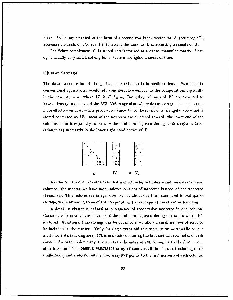
Since PA is implemented in the form of a second row index vector for A (see page 47),

accessing elements of PA (or PV ) involves the same work as accessing elements of A.

The Schur complement C is stored and factorized as a dense triangular matrix. Since

nd is usually very small, solving for z takes a negligible amount of time.

Cluster Storage

The data structure for W is special, since this matrix is medium dense. Storing it in

conventional sparse form would add considerable overhead to the computation, especially

in the case Ad = a, where W is all dense. But other columns of W are expected to

have a density in or beyond the 25%-50% range also, where dense storage schemes become

more effective on most scalar processors. Since W is the result of a triangular solve and is

stored permuted as Wp, most of the nonzeros are clustered towards the lower end of the

columns. This is especially so because the minimum-degree ordering tends to give a dense

(triangular) submatrix in the lower right-hand corner of L.

* SL = uP

In order to have one data structure that is effective for both dense and somewhat sparser

columns, the scheme we have used indexes clusters of nonzeros instead of the nonzeros

themselves. This reduces the integer overhead by about one third compared to real sparse

storage, while retaining some of the computational advantages of dense vector handling.

In detail, a cluster is defined as a sequence of consecutive nonzeros in one column.

Consecutive is meant here in terms of the minimum-degree ordering of rows in which WP

is stored. Additional time savings can be obtained if we allow a small number of zeros to

be included in the cluster. (Only for single zeros did this seem to be worthwhile on our

machines.) An indexing array ICL is maintained, storing the first and last row index of each

cluster. An outer index array KCW points to the entry of ICL belonging to the first cluster

of each column. The DOUBLE PRECISION array WT contains all the clusters (including those

single zeros) and a second outer index array KWT points to the first nonzero of each column.

55

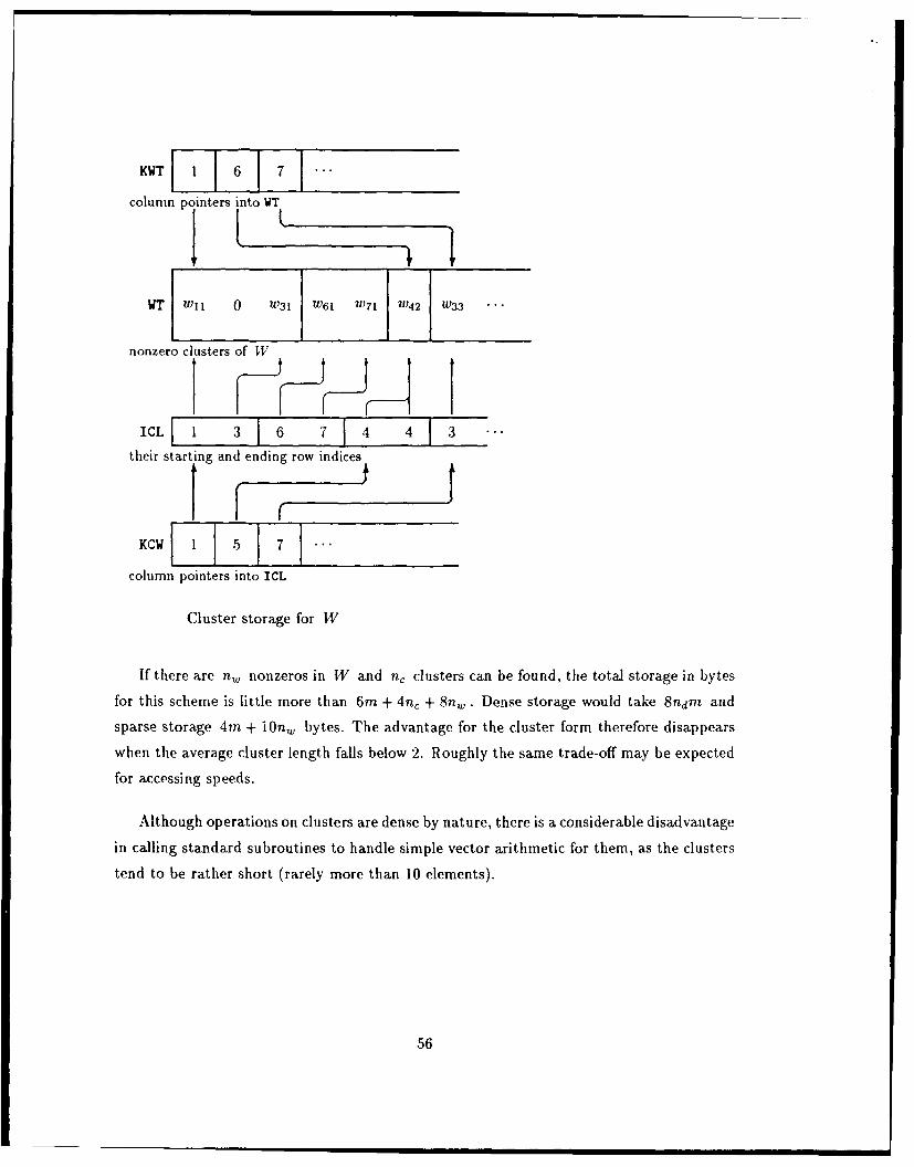
KWT I11 6 1 7

column pointers into WT

I t

I I iICL 1 1 3 16 7 14 4 3 ..

their starting and ending, ro idice

KCW 1 5 1

column pointers into ICL

Cluster storage for W

If there are nw nonzeros in W and n, clusters can be found, the total storage in bytes

for this scheme is little more than 6m + 4n, + 8n,. Dense storage would take 8ndrn and

sparse storage 4m + iOn, bytes. The advantage for the cluster form therefore disappears

when the average cluster length falls below 2. Roughly the same trade-off may be expected

for accessing speeds.

Although operations on clusters are dense by nature, there is a considerable disadvantage

in calling standard subroutines to handle simple vector arithmetic for them, as the clusters

tend to be rather short (rarely more than 10 elements).

56

Chapter 9

The Analyze Phase

The Cholesky factorization of a sparse symmetric positive-definite matrix is a well-studied

problem; see, e.g. [GL81] and [DER86]. The factorization is generally done in two phases,

the Analyze Phase and the Numerical Phase. In the Analyze Phase, the structure uf the

nonzero elements in the matrix is analyzed and a suitable data structure and order of

operations is established. In the Numerical Phase these operations are then executed. For

typical matrices each phase takes about an equal amount of computer time. It is important

to note that the numerical values of the matrix elements are not relevant in the Analyze

Phase. This is true because for positive-definite matrices all orderings are acceptable as far

as numerical stability is concerned.

The systems of equations solved at each iteration of an interior-point methods are a

special application of these factorization techniques. The matrices AH-1AT have the same

nonzero structure for every iteration, independent of the values of H- 1. This leads to a

method that need only have one Analyze Phase and several Numerical Phases. We shall

therefore refer to the Analyze Phase of the barrier algorithm, which performs all non-

numerical setup steps in preparation for forming and factorizing AH-1 A.

Steps of the Analyze Phase include: (1) most importantly, the search for an ordering of

the matrix AH-1AT that reduces the fill-in in its factor L; (2) the sorting of A according to

this ordering; and (3) the generation of data structures for the Schur-complement procedure

to handle dense columns.

The Minimum-Degree Ordering

It is a characteristic of both symmetric and unsymmetric systems that the ordering of rows

and columns has a great deal of influence on the number of nonzeros in the factors, although

it does not change the number of nonzeros in the original matrix. Despite the existence of

57

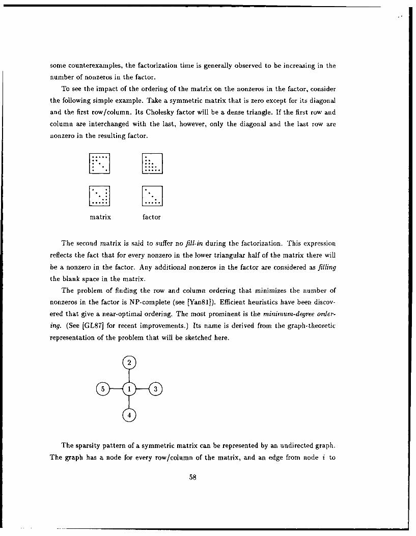
some counterexamples, the factorization time is generally observed to be increasing in the

number of nonzeros in the factor.

To see the impact of the ordering of the matrix on the nonzeros in the factor, consider

the following simple example. Take a symmetric matrix that is zero except for its diagonal

and the first row/column. Its Cholesky factor will be a dense triangle. If the first row and

column are interchanged with the last, however, only the diagonal and the last row are

nonzero in the resulting factor.

matrix factor

The second matrix is said to suffer no fill-in during the factorization. This expression

reflects the fact that for every nonzero in the lower triangular half of the matrix there will

be a nonzero in the factor. Any additional nonzeros in the factor are considered as filling

the blank space in the matrix.

The problem of finding the row and column ordering that minimizes the number of

nonzeros in the factor is NP-complete (see [Yan8l]). Efficient heuristics have been discov-

ered that give a near-optimal ordering. The most prominent is the minimum-degree order-

ing. (See [GL87] for recent improvements.) Its name is derived from the graph-theoretic

representation of the problem that will be sketched here.

2

5 1 3

4

The sparsity pattern of a symmetric matrix can be represented by an undirected graph.

The graph has a node for every row/column of the matrix, and an edge from node i to

58

node j wherever there is a nonzero at (i,j). The graph representation of our example

above is thus a star with node 1 at its center.

The graph equivalent to computing column j of the factor is removing node j from

the graph and adding an edge (i,k) for every pair of nodes i and k that were previously

connected to node j by edges (i,j) and (j,k). The new edge (i,k) corresponds to fill-in

in the factor, if the nodes i and k have not been connected before.

In order to minimize fill-in, i.e., to minimize the number of edges added, the node

with the minimum number of outgoing edges is removed first. Since the number of adjacent

edges is also called the degree of a node, this rule constitutes the minimum-degree algorithm.

Variants of the algorithm differ in the way ties are resolved, and in the frequency with which

the degree is recomputed.

In our little example the minimum-degree algorithm will yield an ordering where node 1

is either last or second to last. All such orderings are optimal. This is due to the fact that

the original graph was a tree, but in general we would not expect the minimum-degree

ordering to generate the least fill-in possible.

The reason for the popularity of the minimum-degree algorithm lies both in the quality

of the resulting ordering and in the efficiency of some of its implementations. (The version

used in our implementation is SPARSPAK's GENHND routine, using a "multiple minimum

external degree" method.) This is to imply that the minimum-degree algorithm was found

to be the best trade-off between the time invested in the Analyze Phase and the time saved

during the Numerical Phase. However, most research in this area assumes that only one

Numerical Phase is performed per Analyze Phase. For the case of interior-point methods,

there is some potential for more expensive ordering methods in the Analyze Phase, since

their cost is amortized over a greater number of factorizations. Adler et al. [AKRV87 report

some success with a minimum local fill-in method.

Cliques

The normal input format for the ordering algorithm is a list of the row and column indices

for each nonzero in the matrix. The first step of the minimum-degree algorithm is to convert

that list into a data structure that represents the adjacencies of the graph.

In order to generate such a list for A- AT, the locations of nonzeros have to be

determined by forming the symbolic product AA T' The product is symbolic in the sense

that there is no real arithmetic involved, but the nonzero patterns of rows are compared.

59

Forming this symbolic product can be avoided by observing that the graph of AAT

consists of cliques. A clique is a set of nodes where each pair of nodes is connected by an

edge. The graph representing the outer product ajaT is a clique. This clique consists of the

nodes that correspond to the rows of the nonzeros in aj. Since AAT is the sum of outer

products ajaT, its graph representation is the union of the corresponding cliques.

Using a special SPARSPAK input routine, the nonzero structure of AAT is simply

represented by the series of cliques corresponding to the columns of A. Dense columns and

columns corresponding to fixed variables are ignored for this purpose.

Sorting A

Once the row ordering is determined, the formation of AH-1AT in the Numerical Phase can

be made considerably more efficient by sorting A. This is done by reordering the entries

of the arrays A and HA (refer to Chapter 7) so that the nonzeros in each column are in

that permuted order. Since dense columns are not included in the Cholesky factorization,

they do not need to be sorted. Consequently the sorting algorithm does not have to be

sophisticated, because the number of nonzeros to sort per column is small. The time spent

on sorting is almost negligible.

Memory allocation and Data Structures

The memory requirements of the minimum-degree algorithm are considerable and are not

bounded by a reasonable function of the dimensions of A. In some instances the memory

required in the Analyze Phase can exceed that of the Numerical Phase.

All memory left after loading A and allocating space for its overhead storage and the

main vectors is first reserved for the minimum-degree algorithm. After the ordering is found,

the memory is reassigned to the data structure that represents L and its overhead.

Given the ordering, the array HPA of permuted row indices is generated (page 47). The

arrays JA and KArow that allow row-wise access to the nonzeros of A are determined by

searching through all non-dense columns.

With these data structures in place, a symbolic solve LW = Ad is performed to deter-

mine the nonzero structure of W. The columns of W are then searched for clusters and

the corresponding integer arrays are generated.

All additional memory is temporary workspace, i.e., contains arrays that are recomputed

at each iteration. These include the pointers needed during the factorization, the numerical

values of W and C, and some work vectors.

60

Part III Testing

Chapter 10

Test Set and Setting

An implementation was developed to test the various facets of the algorithm discussed

in Parts I and II. Since randomly generated problems prove to give poor insight into the

behavior of a large-scale algorithm, a collection of real-world problems was used as the test

set.

The relative performance of different algorithms always depends somewhat on the hard-

ware and software used for the test. With linear programming, these dependencies seem tobe more critical for interior-point methods than for the simplex method.

In addition to presenting the general results of performance tests, we discuss in thischapter the influence that the test set and the computing environment may have on the

performance.

The Test Problems

The set of test problems consists of the first 53 problems in the netlib collection [Gay85].

They are available via electronic mail and have come to be regarded as a standard bench-

mark for linear programming algorithms. In the following tables, the problems are ordered

according to the number of nonzero elements in A as in [Lus87].

Although 53 problems is a reasonably large set, many of the problems are related. The

performance of -plat,d problems is often correlated. No claim is made that the problems

are typical of LP problems commonly solved. Indeed that the problems ended up in a test

set may be some indication the problems are atypical, i.e., hard to solve by the simplex

method. Too much, therefore, should not be concluded from the results. Batch testing ofthis type is perhaps best viewed as a means for detecting bad algorithms.

Apart from the use of row and column scaling where indicated, each problem was solved

as given. No attempt was made to simplify the problems by first preprocessing them,

61

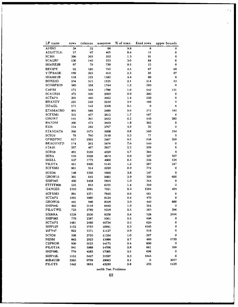
LP name rows columns nonzeros % of nonz. fixed rows upper bounds

AFIRO 28 32 88 9.8 8 0ADLITTLE 57 97 465 8.4 15 0SC205 206 203 552 1.3 91 0SCAGR7 130 140 553 3.0 84 0SHARE2B 97 79 730 9.5 13 0

RECIPE 92 180 752 4.5 67 69VTPBASE 199 203 914 2.3 55 97SHAREIB 118 225 1182 4.4 89 0BORE3D 234 315 1525 2.1 214 12SCORPION 389 358 1744 1.2 280 0

CAPRI 272 353 1786 1.9 142 131SCAGR25 472 500 2029 0.9 300 0SCTAP1 301 480 2052 1.4 120 0

BRANDY 221 249 2150 3.9 166 0ISRAEL 175 142 2358 9.5 0 0

ETAMACRO 401 688 2489 0.9 272 180SCFXM1 331 457 2612 1.7 187 0GROW7 141 301 2633 6.2 140 280BANDM 306 472 2659 1.8 305 0E226 224 282 2767 4.9 33 0

STANDATA 360 1075 3038 0.8 160 104SCSD1 78 760 3148 5.3 77 0GFRDPNC 617 1092 3467 0.5 548 258BEACONFD 174 262 3476 7.6 140 0STAIR 357 467 3857 2.3 209 6

SCRS8 491 1169 4029 0.7 384 0SEBA 516 1028 4874 0.9 507 507SHELL 537 1775 4900 0.5 534 126PILOT4 411 1000 5145 1.2 287 247SCFXM2 661 914 5229 0.9 374 0

SCSD6 148 1350 5666 2.8 147 0GROW15 301 645 5665 2.9 300 600SHIP04S 403 1458 5810 1.0 354 0FFFFF800 525 854 6235 1.4 350 0GANGES 1310 1681 7021 0.3 1284 404

SCFXM3 991 1371 7846 0.6 561 0SCTAP2 1091 1880 8124 0.4 470 0GROW22 441 946 8318 2.0 440 880SHIPo4L 403 2118 8450 1.0 354 0PILOTWE 723 2789 9218 0.5 583 296

SIERRA 1228 2036 9338 0.4 528 2016SHIP08S 779 2387 9501 0.5 698 0SCTAP3 1481 2480 10734 0.3 620 0SHIP12S 1152 2763 10941 0.3 1045 025FV47 822 1571 11127 0.9 516 0

SCSD8 398 2750 11334 1.0 397 0NESM 663 2923 13988 0.7 480 1739CZPROB 930 3523 14173 0.4 890 0PILOTJA 941 1988 14706 0.8 661 339SHIPO8L 779 4283 17085 0.5 698 0

SHIP12L 1152 5427 21597 0.3 1045 080BAU3B 2263 9799 29063 0.1 0 3057PILOTS 1442 3652 43220 0.8 233 1129

netlib Test Problems

62

e.g., by eliminating redundant constraints. The experiments were intended to investigate

algorithmic performance in precisely the kind of circumstances that such procedures are

designed to eliminate. Preprocessing may prove useful within a practical code. ([AKRV87]

discusses experiences with it.) However, preprocessing cannot be assumed to eliminate

undesirable features of linear programs. This is particularly true for very large problems.

The Computing Environment

All runs were obtained as batch jobs on a DEC VAXstation II. The operating system was

VAX/VMS version 4.5. The compiler was VAX FORTRAN version 4.6 with default options,

including code optimization and D.floating arithmetic (relative precision c. 2.8 x 10-17 ).

Solution times are given in CPU seconds; they do not include time for data input or solution

output.

The simplex implementation used for comparison purposes is the Fortran code MINOS 5.3

(May 1988). Default values of the parameters were used throughout (see [GMSW88]); these

include scaling (SCALE OPTION 2) and partial pricing (PARTIAL PRICE 10). See also Lustig

[Lus87] for a comparison of different parameter settings with MINOS.

Memory Constraints

Our implementation of the primal barrier method was designed to keep paging to a minimum

within the available memory. This is relevant for two reasons. First, the implementation

tests the behavior of an interior-point method in a workstation environment, which recently

has evolved as the computer of choice for many linear programming applications. Sec-

ond, it makes comparisons with the simplex method more meaningful, since MINOS works

comfortably within this memory constraint.

For the largest problem, PILOTS, our implementation requires about 3 megabytes of

in-core memory. That includes one copy of A and L, as well as the necessary vectors and

integer data structures. MINOS requires a little over 2 megabytes to solve PILOTS.

On other machines, there are several opportunities to enhance the speed of the factor-

ization by using more memory. Instead of forming AH-AT and overwriting it by L at

every iteration, it is possible to keep and update AH- AT by adding some A AHI AT. By

using an approximate H - 1, the diagonal of AH -1 may contain many zeros and make the

update A AH - 1AT very sparse and efficient to compute, see [AKRV87]. Another option is

63

to compute and store every product aijaki of nonzeros of a column of A once. Forming

the elements of AII-IAT is then accomplished by multiplying these products with h, - 1 and

adding them up; see [MM87].

Still more memory intensive is the interpretative procedure. At the innermost loop of

the Cholesky factorization are operations of the type

lk = lk - lkjlij.

Since all (i,j, k) combinations for which this operation is nontrivial are known during the

Analyze Phase, the memory locations involved in each of these operations can be recorded in

one very long array. This eliminates a large part of the overhead needed to access the sparse

data structures. Adler et al. [AKRV87] use this method in one part of the factorization,

while treating the other part of L as dense to save memory. Such an approach seems

especially promising for machines with vector-type architecture. However, Gay [Gay88]

reports that the interpretative procedure rarely saves more than 20% of the factorization

time on the netlib test set.

In the short history of research on interior-point methods, several implementations were

developed that exploit the resources of advanced computers to an extent not common in

portable simplex codes. As work on both types of linear programming algorithm continues,

it will be interesting to see whether the ability to make use of such resources will give

interior-point methods an advantage. This research, however, tries to compare the two

using about the same amount of memory and using similar data structures for both.

The Runs

As with the implementation of any other optimization method, many preassigned parame-

ters must be selected. We define a run to be a suite of results for a group of test problems

that were all solved using the same set of parameters.

The table on page 65 reports on a run that includes all 53 problems. The main charac-

teristics are that the problems are solved unscaled, small bounds are added to fixed slack

variables, and the composite objective function uses a fairly small weight w = 10- 4 .

The results are reported in terms of the number of (minor) iterations, the optimal value

of the linear objective function, the norm of infeasibilities in relation to the norm of the so-

lution x, and the solution time. The last two columns give the corresponding solution time

64

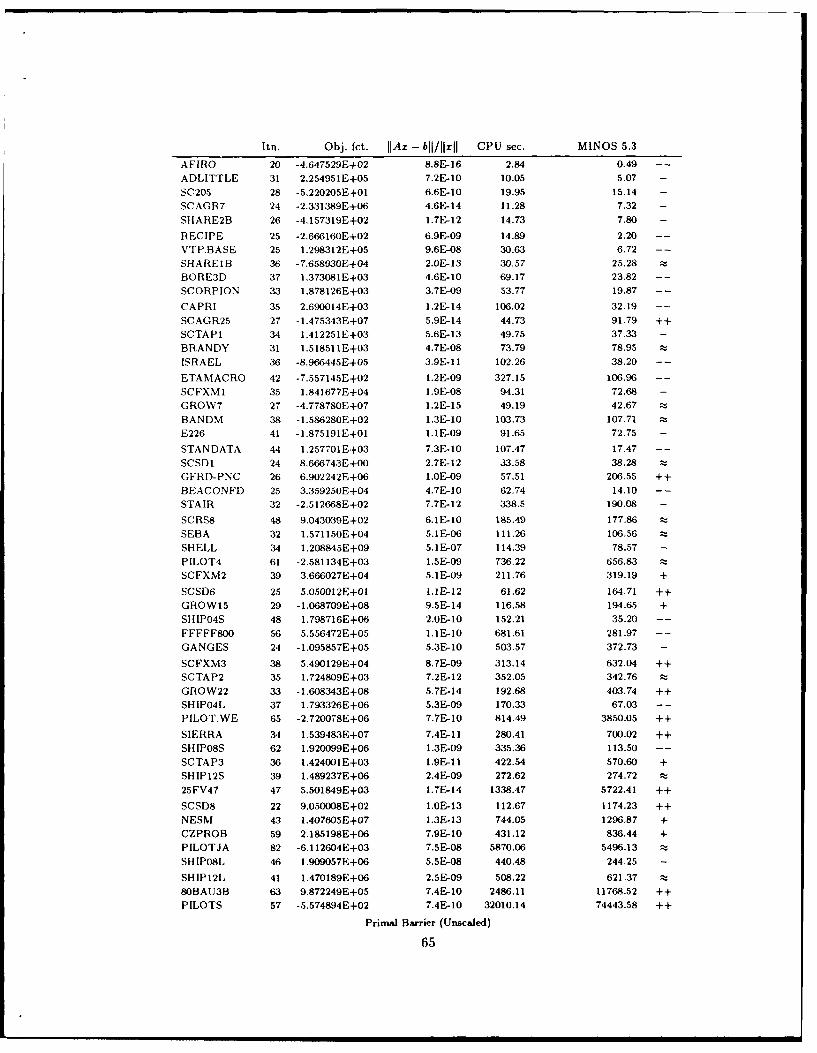
Itn. Obj. fct. lIAz - b1/1111 CPU sec. MINOS 5.3

AFIRO 20 -4.647529E+02 8.8E-16 2.84 0.49 --

ADLITTLE 31 2.254951E+05 7.2E-10 10.05 5.07 -

SC205 28 -5.220205E+01 6.6E-10 19.95 15.14 -

SCAGR7 24 -2.331389E+06 4.6E-14 11.28 7.32 -

SHARE2B 26 -4.157319E+02 1.7E-12 14.73 7.80 -

RECIPE 25 -2,666160E+02 6.9E-09 14.89 2.20 --

VTP.BASE 25 1.298312E+05 9.6E-08 30.63 6.72 --

SHAREIB 36 -7.658930E+04 2.0E-13 30.57 25.28

BORE3D 37 1.373081E+03 4.6E-10 69.17 23.82 --

SCORPION 33 1.878126E+03 3.7E-09 53.77 19.87

CAPRI 35 2.690014E+03 1.2E-14 106.02 32.19 --

SCAGR25 27 -1.475343E+07 5.9E-14 44.73 91.79 ++

SCTAPI 34 1.412251E+03 5.6E-13 49.75 37.33 -

BRANDY 31 1.518511 E+03 4.7F-08 73.79 78.95

ISRAEL 36 -8.966445E+05 3.9- 11 102.26 38.20 --

ETAMACRO 42 -7.557145E+02 1.2E-09 327.15 106.96 --

SCFXM1 35 1.841677E+04 1.9E-08 94.31 72.68 -

GROW7 27 -4.778780E+07 1.2E-15 49.19 42.67

BANDM 38 -1.586280E+02 1.3£-10 103.73 107.71

E226 41 -1.875191E+01 1.1E-09 91.65 72.75 -

STANDATA 44 1.257701E+03 7.3E-10 107.47 17.47 --

SCSDI 24 8.666743E+00 2.7E-12 33.58 38.28

GFRD-PNC 26 6.902242E+06 1.OE-09 57.51 206.55 ++

BEACONFD 25 3.359250E+04 4.7E-10 62.74 14.10 --

STAIR 32 -2.512668E+02 7.7E-12 338.5 190.08 -

SCRS8 48 9.043039E+02 6.1E-10 185.49 177.86

SEBA 32 1.571150E+04 5.1E-06 111.26 106.56

SHELL 34 1.208845E+09 5.1E-07 114.39 78.57 -

PILOT4 61 -2.581134E+03 1.SE-09 736.22 656.83

SCFXM2 39 3.666027E+04 5.1E-09 211.76 319.19 +

SCSD6 25 5.050012E+01 1.1E-12 61.62 164.71 ++

GROWl5 29 -1.068709E+08 9.5E-14 116.58 194.65 +SHIP04S 48 1.798716E+06 2.OE-10 152.21 35.20 --

FFFFF800 56 5.556472E+05 I.E-10 681.61 281.97 --

GANGES 24 -1.095857E+05 5.3E-10 503.57 372.73 -

SCFXM3 38 5.490129E+04 8.7E-09 313.14 632.04 ++SCTAP2 35 1.724809E+03 7.2E-12 352.05 342.76 -,

GROW22 33 - 1.608343E+08 5.7E-14 192.68 403.74 ++

SHIP04L 37 1.793326E+06 5.3E-09 170.33 67.03 --PILOT.WE 65 -2.720078E+06 7.7£-10 814.49 3850.05 ++

SIERRA 34 1.539483E+07 7.4E-11 280.41 700.02 ++

SHIP08S 62 1.920099E+06 1.3E-09 335.36 113.50 --

SCTAP3 36 1.424001E+03 1.9-I 1 422.54 570.60 +

SHIP12S 39 1.489237E+06 2.4E-09 272.62 274.72

25FV47 47 5.501849E+03 1.7E-14 1338.47 5722.41 ++

SCSD8 22 9.050008E+02 1.OE-13 112.67 1174.23 ++

NESM 43 1.407605E+07 1.3E-13 744.05 1296.87 +CZPROB 59 2.185198E+06 7.9E-10 431.12 836.44 +

PILOTJA 82 -6.112604E+03 7.5E-08 5870.06 5496.13

SHIP08L 46 1.909057E+06 5.5E-08 440.48 244.25 -

SHIPI2L 41 1.470189E+06 2.5E-09 508.22 621.37 :

80BAU3B 63 9.872249E+05 7.4E-10 2486.11 11768.52 ++

PILOTS 57 -5.574894E+02 7.4E-10 32010.14 74443.58 ++

Primal Barrier (Unscaled)

65

for MINOS and a comparison category. Based on the ratio p = barrier time/MINOS time,

the categories stand for

++ for (P<0.5

+ for 0.5<4<0.8

for 0.8 < (p < 1.25

- for 1.25< e<2.0

-- for p>2.0.

Some observations may be made that are generally true for all barrier method runs. The

iteration count is low, rarely over 60, and it increases little with the size of the problem. The

barrier times are relatively better for larger problems and are especially good for problems

that are hard to solve for the simplex code.

Failures

As with any other algorithm, if one set of parameters must be chosen for all problems, the

performance is not as good as when the parameters are chosen for a smaller subset of the

problems. The difficulty of choosing an acceptable set of parameters is even greater for

the primal barrier implementation, where both performance and reliability prove to be a

problem. The barrier code using a given set of parameters might fail to solve an LP for a

number of reasons:

* Slow convergence. If the starting point or any other iterate is not sufficiently interior,

the method is likely to take many small steps along the boundary of the feasible region.

We terminate the algorithm at iteration 120 .nd rate such behavior as a failure.

" No Phase II. When the objective weight w is too large, the convergence criteria might

be satisfied before a sufficiently feasible point is found.

* Infeasible termination. Ill-conditioning in Phase II may result in infeasible search

directions, leading to a solution that lies outside of the feasibility tolerance.

* Overflow. Extreme ill-conditioning (and/or insufficient remedies for it) may lead

to floating-point numbers larger than the maximum machine-representable number

during the factorization ( 1.7 x 1038 in the D-floating format).

66

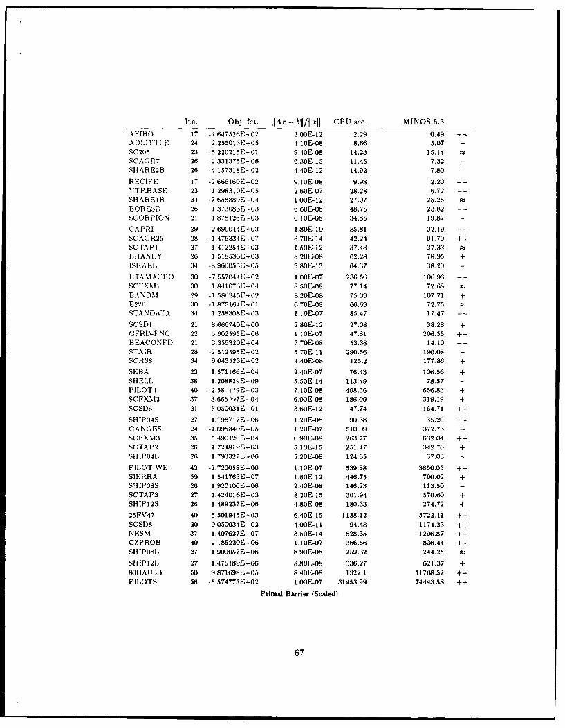
Itni. Obj. fct. ljAx - blI/ljzjl CPU sec. MINOS 5.3

AFIRO 17 -4.647526E+02 3.00E-12 2.29 0.49 -

ADLITTLE 24 2.255013E+05 4.10E-08 8.66 5.07 -

SC205 23 -5.220215E+01 9.40E-08 14.23 15.14SCAGR7 26 -2.331375E+06 6.3oE-i5 11.45 7.32 -

SHIARE2B 26 -4.157318E+02 4.4oE-12 14.92 7.80 -

RECIPE 17 -2.66616oE+02 9.1oE-o8 9.98 2.20"TP.BASE 23 1.298310E+05 2.60E-07 28.28 6.72 -

SHAREIB 34 -7.658889E+04 i.ooE-12 27.07 25.28BORE3D) 26 1.373083E+03 6.60E-08 48.75 23.82 -

SCORPION 21 1.878126E+03 6.10E-08 34.85 19.87 -

CAPRI 29 2.690044E+03 1.80F-10 85.81 32.19 -

S CAGR25 28 -1.475334E+07 3.70E-14 42.24 91.79 ++SCTAPI 27 1.412254E+03 I.5oE-12 37.43 37.33 ;_BRANDY 26 1.518536E+03 8.2oE-08 62.28 78.95 +ISRAEL 34 -8.966053E+05 9.80E-13 64.37 38.20 -

ETANIACRO 30 -7.557044E+02 1.ooE-07 236.56 106.96SCFX%11 30 1.841676E+04 8.50E-08 77.14 72.68BANDIN 29 -1.58/3245E+02 8.20E>08 75.39 107.71 +E226 30 -1.875164E+o1 6.70E-08 66.69 72.75STANDATA 34 1.258308E+03 i.ioE-07 85.47 17.47 -

SCSDI 21 8.666740E+00 2.80E-12 27.08 38.28 +GFRD-PNC 22 6.902595E+06 1.1oE-07 47.81 206.55 ++BEACONFD 21 3.359320E+04 7.70E-08 53.38 14.10 -

STAIR 28 -2.512595E+02 5.7oE-11 290.56 190.08 -

SCRS8 34 9.043523E+02 4.40E-08 125.2 177.86 +

SEBA 23 1.571166E+04 2.40E-07 76.43 106.56 +SHELL 38 1.208A2SoE+09 5.50E- 14 113.49 78.57 -

PILOT4 40 -2.58 11'9E+03 7.10E-08 498.36 656.83 +SCFXN12 37 3.665 ")7E+04 6.90E-08 186.09 319.19 +SCSD6 21 S.050031E+01 3.60E-12 47.74 164.71 ++SHIP04S 27 1.798717E+06 1.20E-08 90.38 35.20 -

GANGES 24 -1.095840E+05 1.20E-07 510.09 372.73 -

SCFXM3 35 5.490126E+04 6.90E-08 263.77 632.04 ++SCTAP2 26 1.724819E+03 5.10E-15 251.47 342.76 +SHIP04L, 26 1.793327E+o6 5.20E-08 124.65 67.03 -

PILOTWE 43 -2.720058E+06 i.10E-07 539.88 3850.05 ++SIERRA 59 1.541763E+07 1.80E-12 446.75 700.02 +S!I IP08S 26 1.920100E+06 2.40F-08 146.23 113.50 -

SCTAP3 27 1.424016E+03 8.20F,15 301.94 570.60 2

SHIP12S 26 1.489237E+06 4.80E-08 180.33 274.72 +25FV47 40 5.501945E+03 6.40E-15 1138.12 5722.41 + +SCSD8 20 9.050034E+02 4.OOE-11 94.48 1174.23 + +NESM 37 1.407627E+07 3.50E-14 628.35 1296.87 + +CZPROB 49 2.185220E+06 1.10F,07 366.56 836.44 + +SHIP08L 27 1.909057E+06 8.90E-08 259.32 244.25

SIIIP12L 27 1.470189E+06 8.80E-08 336.27 621.37 +80BAU3B 50 9.871698E+05 8.40E-08 1922.1 11768.52 ++PILOTS 56 -5.574775E+02 1.OOE-07 31453.99 74443.58 ++

Primal Barrier (Scaled)

67

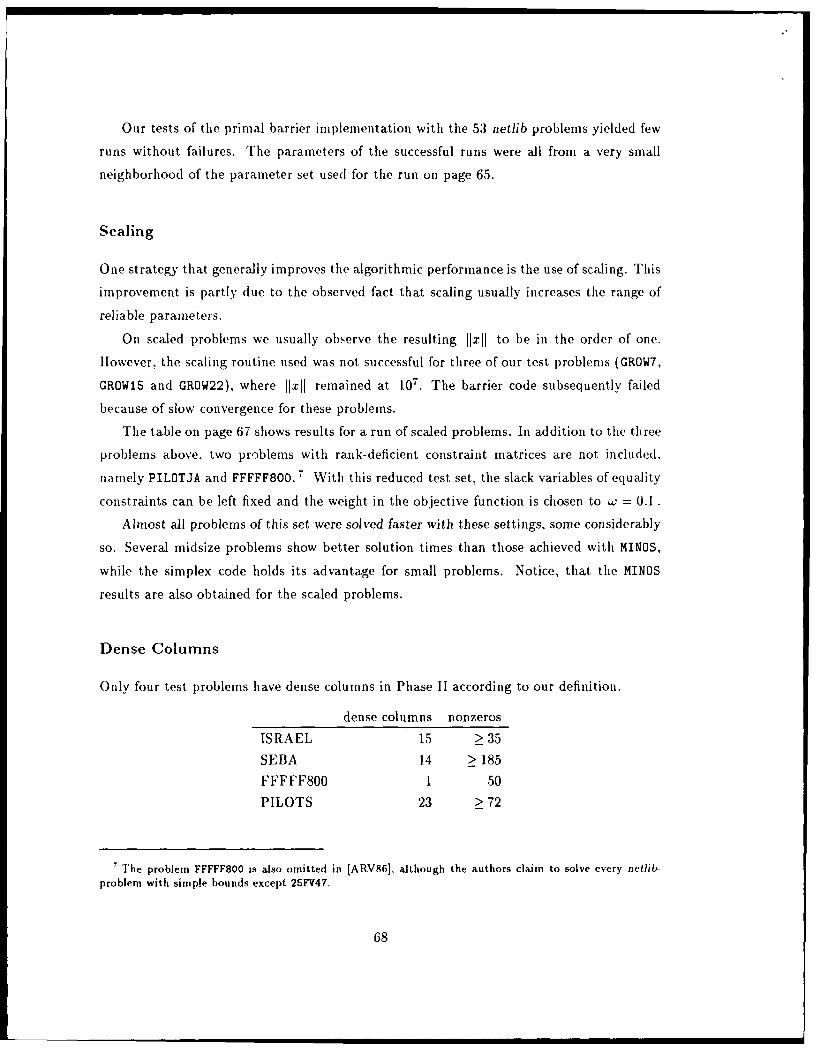
Our tests of the primal barrier implementation with the 53 netlib problems yielded few

runs without failures. The parameters of the successful runs were all from a very small

neighborhood of the parameter set used for the run on page 65.

Scaling

One strategy that generally improves the algorithmic performance is the use of scaling. This

improvement is partly due to the observed fact that scaling usually increases the range of

reliable parameters.

On scaled problems we usually observe the resulting II[xH to be in the order of one.

However, the scaling routine used was not successful for three of our test problems (GROW7,

GROWLS and GROW22), where lixli remained at 107. The barrier code subsequently failed

because of slow convergence for these problems.

The table on page 67 shows results for a run of scaled problems. In addition to the three

problems above, two problems with rank-deficient constraint matrices are not included,

namely PILOTJA and FFFFF800. With this reduced test set, the slack variables of equality

constraints can be left fixed and the weight in the objective function is chosen to W = 0.1.

Almost all problems of this set were solved faster with these settings, some considerably

so. Several midsize problems show better solution times than those achieved with MINOS,

while the simplex code holds its advantage for small problems. Notice, that the MINOS

results are also obtained for the scaled problems.

Dense Columns

Only four test problems have dense columns in Phase II according to our definition.

dense columns nonzeros

ISRAEL 15 > 35

SEBA 14 > 185

FFFFF800 1 50

PILOTS 23 > 72

7 The problem FFFFF800 is also omitted in [ARV86], although the authors claim to solve every netlib-problem with simple bounds except 25FV47.

68

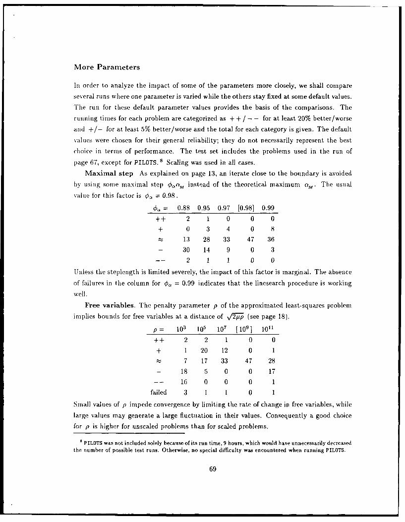
More Parameters

In order to analyze the impact of some of the parameters more closely, we shall compare

several runs where one parameter is varied while the others stay fixed at some default values.

The run for these default parameter values provides the basis of the comparisons. The

running times for each problem are categorized as + + / - - for at least 20% better/worse

and +/- for at least 5% better/worse and the total for each category is given. The default

values were chosen for their general reliability; they do not necessarily represent the best

choice in terms of performance. The test set includes the problems used in the run of

page 67, except for PILOTS. 8 Scaling was used in all cases.

Maximal step As explained on page 13, an iterate close to the boundary is avoided

by using some maximal step 0,,a, instead of the theoretical maximum aM. The usual

value for this factor is , = 0.98.

= 0.88 0.95 0.97 [0.98] 0.99

++ 2 1 0 0 0

+ 0 3 4 0 8

13 28 33 47 36

- 30 14 9 0 3

-- 2 1 1 0 0

Unless the steplength is limited severely, the impact of this factor is marginal. The absence

of failures in the column for C. = 0.99 indicates that the linesearch procedure is working

well.

Free variables. The penalty parameter p of the approximated least-squares problem

implies bounds for free variables at a distance of 2)u (see page 18).

p = 103 10 107 [109] 1011

++ 2 2 1 0 0

+ 1 20 12 0 1

7 17 33 47 28

- 18 5 0 0 17

16 0 0 0 1

failed 3 1 1 0 1

Small values of p impede convergence by limiting the rate of change in free variables, while

large values may generate a large fluctuation in their values. Consequently a good choice

for p is higher for unscaled problems than for scaled problems.

8 PILOTS was not included solely because of its run time, 9 hours, which would have unnecessarily decreasedthe number of possible test runs. Otherwise, no special difficulty was encountered when running PILOTS.

69

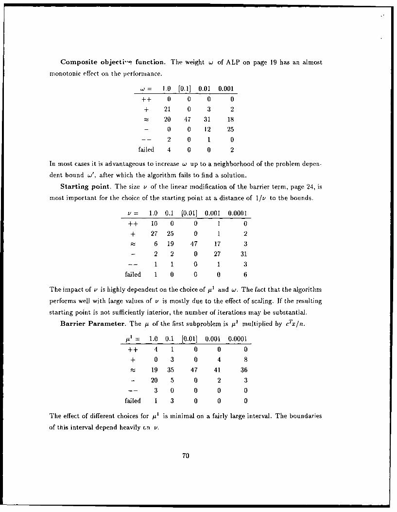
Composite objecti-- function. The weight w of ALP on page 19 has an almost

monotonic effect on the performance.

.,= 1.0 [0.1] 0.01 0.001

++ 0 0 0 0

+ 21 0 3 2

20 47 31 18

- 0 0 12 25-- 2 0 1 0

failed 4 0 0 2

In most cases it is advantageous to increase w up to a neighborhood of the problem depen-

dent bound w, after which the algorithm fails to find a solution.

Starting point. The size v of the linear modification of the barrier term, page 24, is

most important for the choice of the starting point at a distance of 1/v to the bounds.

V = 1.0 0.1 [0.011 0.001 0.0001

++ 10 0 0 1 0

+ 27 25 0 1 2

6 19 47 17 3

- 2 2 0 27 31

-- 1 1 0 1 3

failed 1 0 0 0 6

The impact of v is highly dependent on the choice of pi and w. The fact that the algorithm

performs well with large values of v is mostly due to the effect of scaling. If the resulting

starting point is not sufficiently interior, the number of iterations may be substantial.

Barrier Parameter. The ju of the first subproblem is /i1 multiplied by cTx/n.

A1 = 1.0 0.1 [0.01] 0.001 0.0001

++ 4 1 0 0 0

+ 0 3 0 4 8

. 19 35 47 41 36

- 20 5 0 2 3

-- 3 0 0 0 0

failed 1 3 0 0 0

The effect of different choices for pl is minimal on a fairly large interval. The boundaries

of this interval depend heavily rn v.

70

Bibliography

[AKRV87] I. Adler, N. Karmarkar, M. G. C. Resende and G. Veiga (1987). Data struc-

tures and programming techniques for the implementation of Karmarkar's

algorithm, Manuscript (December 1987), Department of Industrial Engineer-

ing and Operations Research, University of California, Berkeley, CA.

[ARV861 1. Adler, M. G. C. Resende and G. Veiga (1986). An implementation of Kar-

markar's algorithm for linear programming, Report ORC 86-8, Department

of Industrial Engineering and Operations Research, University of California,

Berkeley, CA.

[Bj87a] A. Bjorck (1987). Stability analysis of the method of semi-normal-equations

for linear least-squares problems, Linear Algebra and its Applications, 88/89,

31-48.

[Bj87b] A. Bjorck (1987). Iterative refinement and reliable computing, Advances in

Reliable Numerical Computing, M. Cox and S. J. Hammarling, ed., Oxford

University Press.

[Brent73] R. P. Brent (1973). Algorithms for Minimization without Derivatives, Pren-

tice-Hall, Englewood Cliffs, NJ.

[CGLN84] E. Chu, J. A. George, J. W. H. Liu and E. Ng (1984). SPARSPAK: Waterloo

Sparse Matrix Package User's Guide for SPARSPAK-A, Report CS-84-36,

Department of Computer Science, University of Waterloo, Waterloo, Canada.

[Dan63] G. B. Dantzig (1963). Linear Programming and Extensions, Princeton Uni-

versity Press, Princeton, New Jersey.

[DER86] I. S. Duff, A. M. Erisman and J. K. Reid (1986). Direct Methods for Sparse

Matrices, Clarendon Press, Oxford, England.

71

[Dik67] I. I. Dikin (1967). Iterative solution of problems of linear and quadratic pro-

gramming, Doklady Akademii Nauk SSSR, Tom 174, No. 4.

[Fia79] A. V. Fiacco (1979). Barrier methods for nonlinear programming, in A. Holz-

man (ed.), Operations Research Support Methodology, Marcel Dekker, Inc.,

New York, 377-440.

[FM68] A. V. Fiacco and G. P. McCormick (1968). Nonlinear Programming: Sequen-

tial Unconstrained Minimization Techniques, John Wiley and Sons, New York

and Toronto.

[Fle8l] R. Fletcher (1981). Practical Methods of Optimization, Volume 2, John Wiley

and Sons, Chichester and New York.

[FM69] R. Fletcher and A. P. McCann (1969). Acceleration techniques for nonlinear

programming, in: R. Fletcher, ed., Optimization, Academic Press, London,

203-213.

[Fri54] K. R. Frisch (1954). Principles of linear programming-with particular refer-

ence to the double gradient form of the logarithmic barrier function, Memo-

randum, University Institute of Economics, Oslo, Norway.

[Fri57] K. R. Frisch (1957). Linear dependencies and a mechanized form of the multi-

plex method for linear programming, University Institute of Economics, Oslo,

Norway.

[Gay85] D. M. Gay (1985). Electronic mail distribution of linear programming test

problems, Mathematical Programming Society COAL Newsletter 13, 10-12.

[Gay88] D. M. Gay (1988). Massive memory buys little speed for complete, in-core

sparse Cholesky factorizations, Numerical Analysis Manuscript 88-04, AT&T

Bell Laboratories, Murray Hill, NJ 07974.

[GL81] J. A. 3eorge and J. W. H. Liu (1981). Computer Solution of Large Sparse

Positive Definite Systems, Prentice-Hall, Englewood Cliffs, NJ.

[GL87] J. A. George and J. W. H. Liu (1987). The evolution of the minimum degree

ordering algorithm, ORNL/TM-10452, Oak Ridge National Laboratory, Oak

Ridge, TN.

72

(GLN88] J. A. George, J. W. H. Liu and E. Ng (1988). A data structure for sparse QR

and LU factorizations, SIAM J. on Scientific and Statistical Computing 9,

100-121.

[GMSTW86] P. E. Gill, W. Murray, M. A. Saunders, J. A. Tomlin and M. H. Wright

(1986). On projected Newton barrier methods for linear programming and an

equivalence to Karmarkar's projective method, Mathematical Programming

36, 183-209.

[GMSW84] P. E. Gill, W. Murray, M. A. Saunders and M. H. Wright (1984). Sparse matrix

methods in optimization, SIAM J. on Scientific and Statistical Computing 5,

562-589.

[GMSW86] P. E. Gill, W. Murray, M. A. Saunders and M. H. Wright (1986). A note on

nonlinear approaches to linear programming, Report SOL 86-7, Department

of Operations Research, Stanford University, Stanford, CA.

[GMSW88] P. E. Gill, W. Murray, M. A. Saunders and M. H. Wright (1988). A practical

anti-cycling procedure for linear and nonlinear programming, Report SOL 88-

4, Department of Operations Research, Stanford University, Stanford, CA.

[GMW81] P. E. Gill, W. Murray and M. H. Wright (1981). Practical Optimization,

Academic Press, London and New York.

[GN84] J. A. George and E. Ng (1984). SPARSPAK: Waterloo sparse matrix package

user's guide for SPARSPAK-B, Report CS-84-37, Department of Computer

Science, University of Waterloo, Waterloo, Canada.

[Gon87] C. C. Gonzaga (1987). Search directions for interior linear programming meth-

ods, Memorandum UCB/ERL M87/44, Electronics Research Laboratory, Col-

lege of Engineering, University of California, Berkeley, CA.

[GVL83] G. H. Golub and C. F. Van Loan (1983). Matrix Computations, The Johns

Hopkins University Press, Baltimore, MA.

[HS52] M. R. Hestenes and E. Stiefel (1952). Methods of conjugate gradients for

solving linear systems, J. Res. Nat. Bur. Stand. 49, 409-436.

[Jit78] K. Jittorntrum (1978). Sequential Algorithms in Nonlinear Programming,

Ph. D. Thesis, Australian National University, Canberra, Australia.

73

[J078] K. Jittorntrum and M. R. Osborne (1978). Trajectory analysis and extrapola-

tion in barrier function methods, Journal of Australian Mathematical Society

20 (Series B) 352-369.

[Kar84] N. K. Karmarkar (1984). A new polynomial-time algorithm for linear pro-

gramming, Combinatorica 4, 373-395.

[KR88] N. K. Karmarkar and K. G. Ramakrishnan (1988). Implementation and com-

putational results of the Karmarkar algorithm for linear programming, us-

ing an iterative method for computing projections, extended abstract for the

Mathematical Programming Symposium, Tokyo, Japan.

[Kha79] L. G. Khachiyan (1979). A polynomial algorithm in linear programming, Dok-

lady Akademii Nauk SSSR Novaia Seriia 244, 1093-1096. [English translation

in Soviet Mathematics Doklady 20, 191-194.]

[Lus87] I. J. Lustig (1987). An analysis of an available set of linear programming test

problems, Report SOL 87-11, Department of Operations Research, Stanford

University, Stanford, CA.

[Mon87I C. L. Monma (1987). Recent breakthroughs in linear programming methods,

Manuscript, Bell Communications Research, Morristown, NJ.

[MM87] C. L. Monma and A. J. Morton (1987). Computational experience with a

dual affine variant of Karmarkar's method for linear programming, Operations

Research Letters 6, 261-267.

[MA87] R. D. C. Monteiro and I. Adler (1987). Interior path following primal-dual

algorithms-Part I: Linear programming, Technical Report, Department of

Industrial Engineering and Operations Research, University of California,

Berkeley, CA.

[MS83] B. A. Murtagh and M. A. Saunders (1983). MINOS 5.0 user's guide, Report

SOL 83-20, Department of Operations Research, Stanford University, Stan-

ford, CA.

[MW76] W. Murray and M. H. Wi1right (1976). Efficient linear search algorithms for the

logarithmic barrier function, Report SOL 76-18, Department of Operations

Research, Stanford University, Stanford, CA.

74

[Osb72] M. R. Osborne (1972). Topics in Optimization, Report CS-72-279, Computer

Science Department, Stanford University, Stanford, CA.

(PS82] C. C. Paige and M. A. Saunders (1982). LSQR: An algorithm for sparse

linear equations and sparse least squares, ACM Transactions on Mathematical

Software 8, 43-71.

[Par6l] G. R. Parisot (1961). Rdsolution Num6rique Approch6e du Probl~me du Pro-

grammation Lineaire par Application de la Programmation Logarithmique,

Ph. D. Thesis, University of Lille, France.

[RS88] J. Renegar and M. Shub (1988). Simplified complexity analysis for Newton

LP methods, Technical Report No. 807, School of Operations Research and

Industrial Engineering, Cornell University, Ithaca, NY.

[Shor77] N. Z. Shor (1977). The cut-off method with space dilation for solving convex

programming problems, Kibernetika 13, No. 1, 94-95. [English translation in

Cybernetics 13 (1978), 94-96.]

[Stew87] G. W. Stewart (1987). An iterative method for solving linear inequalities.

Report TR-1833, Department of Computer Science, University of Maryland,

College Park, MD.

[Van89] R. J. Vanderbei (1989). Affine-scaling for linear programs with free variables,

Mathematical Programming 43, 31-44.

[VMF86] R. J. Vanderbei, M. S. Meketon and B. A. Freedman (1986). A modification

of Karmarkar's linear programming algorithm, Algorithmica 1, 395-407.

[VLo85] C. F. Van Loan (1985). On the method of weighting for equality-constrained

least-squares problems, SIAM Journal on Numerical Analysis 22, 851-864.

[Wri76] M. 11. Wright (1976). Numerical methods for nonlinearly constrained opti-

mization, Report CS-76-566, Computer Science Department, Stanford Uni-

versity, Stanford, CA.

[Yan8l] M. Yannakakis (1981). Computing the minimum fill-in is NP-complete, SL4AM

J. Alg. & Disc. Math., vol. 2, pp. 77-79.

75

UNCLASSIFIEDSECURITY CLAWMIICATION OF THIS PAGE (900 O0.8101 __________________

REPORT DOCUMENTAT1ON PAGE RA H Unw

REPOR MUME 4 ACCUSSMNO 00 CIPSEM S$ CAT ALOGM ummim

SOL 89-6rATITLE (god &*Muj S TYPE OF REPONT a PCRO COVERZO

Primal Barrier methods for Linear Programming Technical______Report___

S. PaRFORKmMG 04G. REPORT Mumma"

7. AUTWOfR(m) I. COmNTRACT ON 6RANT NUMS9111(s

Aeneas Marxen NOOO1 4-87-K-Cl 42

9. PERFORlMG ORGANIZATION MAWC ANO ADORESS IS. PGSLAM I "MEM1,,P RCT. TASKDepartment of Operations Research - SOLA& 0 MTt

StanforA' University 1111 MAStanforu, CA 94305-4022

11. CO TOOSL WHO OFPPICE M AM AMD ADDRESIS IL 49E0ORTDATE

Office of Naval Research - Dept. of the Navy June 1989800 N. Quincy Street 75 pagestOFPACArlington, VA 22217 5 paUgeYCLsS(. enp

UNCLASSIFIEDI"a :CHMSUUCATOW OUWRAIM@

-16. DISTRIBUTION STATEmENT (of W ma. aw

This document has been approved for public release and sale;its distribution is unlimited.

17. OSR~TO TTMN . e.m mM3.bMi ~n ~8e

10. SUPPLEMENTARY MOTES

19. KEy WORDS (CO M .,wee OW 9 6900sI K p~ Abe was* hI

Linear Programming, Barrier Functions, Cholesky's Algorithm,Sparse Matrices.

M4 AUSTRACT (Cd - inwmes edo Uaeeepr amil U IV Wek6u

(see reverse side)

DO I FAN 7 1473 EDITION OP I Nov IsI OUSOLETE

SECU~IFT CLASIFICATION OP T141 PAGE (fmf Due CLu,

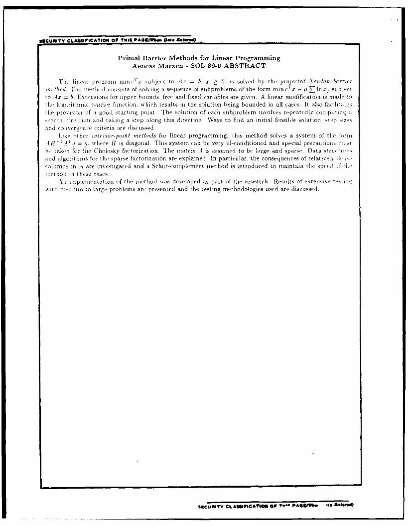
IICumTY CLAWPICAT ION OF THiS PAG1[(Cllw Doa m

Primal Barrier Methods for Linear ProgrammingAeneas Marxen - SOL 89-6 ABSTRACT

The linear progran minJ subject to _-Ix = b. r > 0, is solved by the projected .Vewton barrier,nethod Fie iiethod consists of solving a sequence of subproblems of the form min cTx - a E In x subject.to -Ax = b Extensions for tipper bounds, free and fixed variables are given. A linear modification is made tothe logarithmic barrier function, which results in the solution being bounded in all cases. It also facilitatesthe provision of a good starting point. The solution of each subproblem involves repeatedly coniput ing asearch direct ion and taking a step along this direction. Ways to find an initial feasible solution. step size.sand convergence criteria are discussed.

Like other inlerior-poznt methods for linear programming, this method solves a system of the formAH-.-4q y. where H is diagonal. This system can be very ill-conditioned and special precautions iUtbe taken for the Cholesky factorization. The matrix A is assumed to bc large and sparse. Data structuro0and algorithms for the sparse factorization are explained. In particular, the consequences of relatively ,ril.columns in .4 are investigated and a Schur-complement method is introduced to maintain the speed .f 0.,method in these cases.

An implementation of the method was developed as part of the research. Results of extensive test ingwith inedium to large problems are presented and the testing methodologies used are discussed.

ISOCURIY CLASUPICA 1ON OF Vw*v PAGCO4Uh. * ZnE..,E