Embed Size (px)
Citation preview
1
The Geometry–Algebra Dictionary
In this chapter, we will explore the correspondence between alge-
braic sets in affine and projective space and ideals in polynomial
rings. More details and all proofs not given here can be found in
[Decker and Schreyer (to appear)]. We will work over a field K.
All rings considered are commutative with identity element 1.
1.1 Affine Algebraic Geometry
Our discussion of the geometry–algebra dictionary starts with Hil-
bert’s basis theorem which is the fundamental result about ideals
in polynomial rings. Then, focusing on the affine case, we present
some of the basic ideas of algebraic geometry, with particular em-
phasis on computational aspects.
1.1.1 Ideals in Polynomial Rings
To begin, let R be any ring.
Definition 1.1.1 A subset I ⊂ R is called an ideal of R if the
following holds:
(i) 0 ∈ I.
(ii) If f, g ∈ I, then f + g ∈ I.
(ii) If f ∈ R and g ∈ I, then f · g ∈ I.
13
14 The Geometry–Algebra Dictionary
Example 1.1.2
(i) If T ⊂ R is any subset, then all linear combinations g1f1+
· · ·+ grfr, with g1, . . . .gr ∈ R and f1, . . . , fr ∈ T , form an
ideal 〈T 〉 of R, called the ideal generated by T . We also
say that T is a set of generators for the ideal.
(ii) If {Iλ} is a family of ideals of R, then the intersection⋂λ Iλ is also an ideal of R.
(ii) The sum of a family of ideals {Iλ} of R, written∑
λ Iλ,
is the ideal generated by the union⋃
λ Iλ.
Now, we turn to the polynomial ring in n variables x1, . . . , xn with
coefficients in the field K.
Theorem 1.1.3 (Hilbert’s Basis Theorem) Every ideal of the
polynomial ring K[x1, . . . , xn] has a finite set of generators.
Starting with Hilbert’s original proof [Hilbert (1890)], quite a
number of proofs for the basis theorem have been given (see, for
instance, [Greuel and Pfister (2007)] for a brief proof found in the
1970’s). A proof which nicely fits with the spirit of these notes is
due to Gordan [Gordan (1899)]. Though the name Grobner bases
was coined much later by Buchberger†, it is Gordan’s paper in
which these bases make their first appearance. In fact, Gordan
already makes use of the key idea behind Grobner bases which is
to reduce problems concerning arbitrary ideals in polynomial rings
to problems concerning monomial ideals. The latter problems are
usually much easier.
Definition 1.1.4 A monomial in x1, . . . , xn is a product xα =
xα11 · · ·xαn
n , where α = (α1, . . . , αn) ∈ Nn. A monomial ideal of
K[x1, . . . , xn] is an ideal generated by monomials.
The first step in Gordan’s proof of the basis theorem is to show
that monomial ideals are finitely generated (somewhat mistak-
enly, this result is often assigned to Dickson and therefore named
Dickson’s lemma):
† Grobner was Buchberger’s thesis advisor. In his thesis, Buchberger devel-oped his algorithm for computing Grobner bases. See [Buchberger (1965)].
1.1 Affine Algebraic Geometry 15
Lemma 1.1.5 (Dickson’s Lemma) Let A ⊂ Nn be a subset of
multiindices, and let I be the ideal I = 〈xα | α ∈ A〉. Then there
exist α(1), . . . , α(r) ∈ A such that I = 〈xα(1)
, . . . , xα(r) 〉.
Proof We do induction on n, the number of variables. If n = 1,
let α(1) := min{α | α ∈ A}. Then I = 〈xα(1) 〉.Now, let n > 1 and assume that the lemma holds for n− 1.
Given α = (α1, . . . , αn) ∈ Nn, we write α = (α, αn) with α =
(α1, . . . , αn−1). Accordingly, we write xα = xα11 · · ·xαn−1
n−1 .
Let A = {α ∈ Nn−1 | (α, k) ∈ A for some k}, and let J =
〈{xα}α∈A〉 ⊂ K[x1, . . . , xn−1]. By the induction hypothsis, there
exist multiindices β(1) = (β(1)
, β(1)n ), . . . , β(s) = (β
(s), β
(s)n ) ∈ A
such that J = 〈xβ(1)
, . . . , xβ(s)
〉. Let ` = maxj
{β(j)n }. For i =
0, . . . , `, let Ai = {α ∈ Nn−1 | (α, i) ∈ A} and Ji = 〈{xα}α∈Ai〉 ⊂
K[x1, . . . , xn−1]. Using once more the induction hypothesis, we
get β(1)i = (β
(1)
i , i), . . . , β(si)i = (β
(si)
1 , i) ∈ A such that Ji =
〈xβ(1)i , . . . , xβ
(si)
i 〉. Let
B =`∪
i=0{β(1)
i , . . . , β(si)i }.
Then, by construction, every monomial xα, α ∈ A, is divisible by
a monomial xβ , β ∈ B. Hence, I = 〈{xβ}β∈B〉.
In Section 2.1, we will follow Gordan and use Grobner bases to
deduce the basis theorem from the special case treated above.
Theorem 1.1.6 Let R be a commutative ring with 1. The follow-
ing are equivalent:
(i) Every ideal of R is finitely generated.
(ii) (Ascending chain condition) Every chain
I1 ⊂ I2 ⊂ I3 ⊂ . . .
of ideals of R is eventually stationary. That is,
Im = Im+1 = Im+2 = . . . for some m ≥ 1.
Definition 1.1.7 A ring satisfying the equivalent conditions above
is called a Noetherian ring.
16 The Geometry–Algebra Dictionary
1.1.2 Affine Algebraic Sets
Following the usual habit of algebraic geometers, we write An(K)
instead of Kn: The affine n-space over K is the set
An(K) ={(a1, . . . , an) | a1, . . . , an ∈ K
}.
Each polynomial f ∈ K[x1, . . . , xn] defines a function
f : An(K) → K, (a1, . . . , an) 7→ f(a1, . . . , an),
which is called a polynomial function on An(K). Viewing f as
a function allows us to talk about the zeros of f . More generally,
we define:
Definition 1.1.8 If T ⊂ K[x1, . . . , xn] is any set of polynomials,
its vanishing locus (or locus of zeros) in An(K) is the set
V(T ) = {p ∈ An(K) | f(p) = 0 for all f ∈ T}.
Every such set is called an affine algebraic set.
It is clear that V(T ) coincides with the vanishing locus of the ideal
〈T 〉 generated by T . Consequently, every algebraic set A in An(K)
is of type V(I) for some ideal I of K[x1, . . . , xn]. By Hilbert’s ba-
sis theorem, A is the vanishing locus V(f1, . . . , fr) =⋂r
i=1 V(fi)
of a set of finitely many polynomials f1, . . . , fr. Referring to the
vanishing locus of a single nonconstant polynomial as a hyper-
surface in An(K), this means that a subset of An(K) is algebraic
iff it can be written as the intersection of finitely many hypersur-
faces. Hypersurfaces in An(K) are called plane curves.
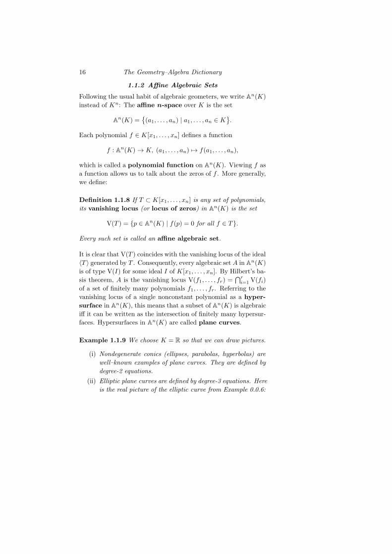
Example 1.1.9 We choose K = R so that we can draw pictures.
(i) Nondegenerate conics (ellipses, parabolas, hyperbolas) are
well–known examples of plane curves. They are defined by
degree-2 equations.
(ii) Elliptic plane curves are defined by degree-3 equations. Here
is the real picture of the elliptic curve from Example 0.0.6:
1.1 Affine Algebraic Geometry 17
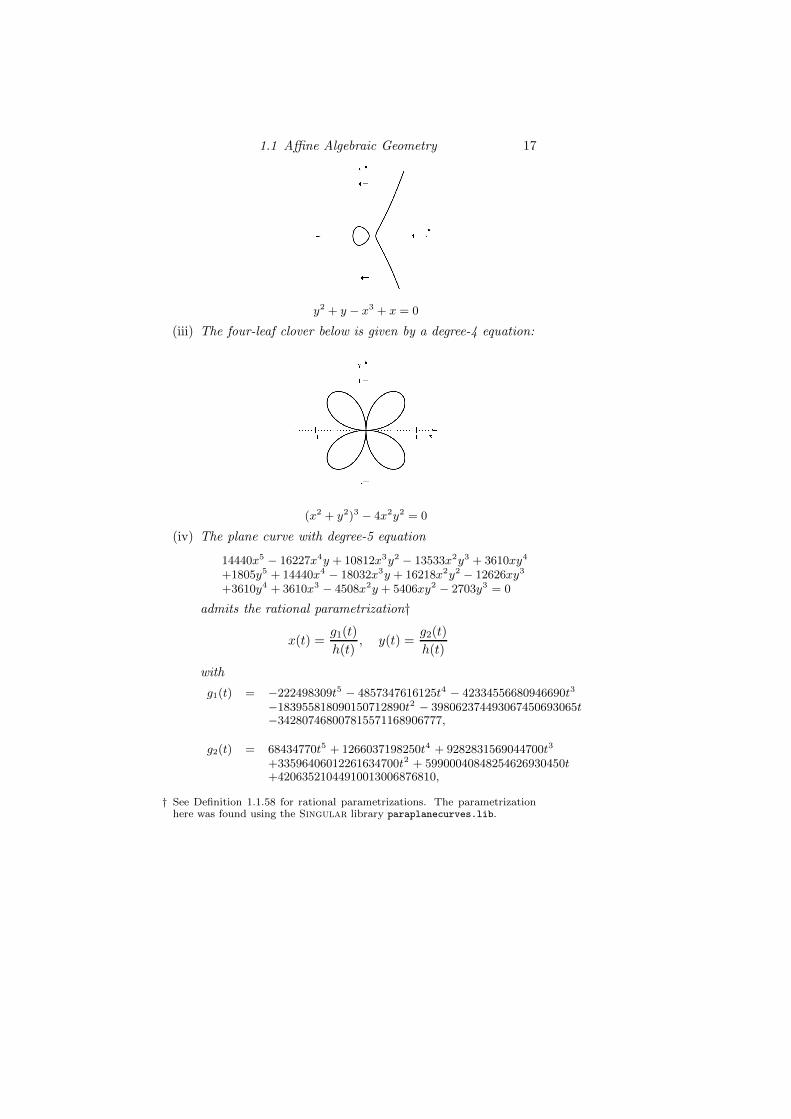
y2 + y − x3 + x = 0
(iii) The four-leaf clover below is given by a degree-4 equation:
(x2 + y2)3 − 4x2y2 = 0
(iv) The plane curve with degree-5 equation
14440x5 − 16227x4y + 10812x3y2 − 13533x2y3 + 3610xy4
+1805y5 + 14440x4 − 18032x3y + 16218x2y2 − 12626xy3
+3610y4 + 3610x3 − 4508x2y + 5406xy2 − 2703y3 = 0
admits the rational parametrization†
x(t) =g1(t)
h(t), y(t) =
g2(t)
h(t)
with
g1(t) = −222498309t5 − 4857347616125t4 − 42334556680946690t3
−183955818090150712890t2 − 398062374493067450693065t−342807468007815571168906777,
g2(t) = 68434770t5 + 1266037198250t4 + 9282831569044700t3
+33596406012261634700t2 + 59900040848254626930450t+42063521044910013006876810,
† See Definition 1.1.58 for rational parametrizations. The parametrizationhere was found using the Singular library paraplanecurves.lib.
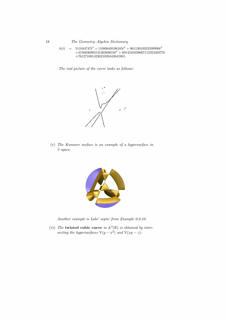
18 The Geometry–Algebra Dictionary
h(t) = 511044747t5 + 11089849198185t4 + 96113019353599990t3
+415003698313126569610t2 + 891424503866711235249375t+761271081423021028442641901.
The real picture of the curve looks as follows:
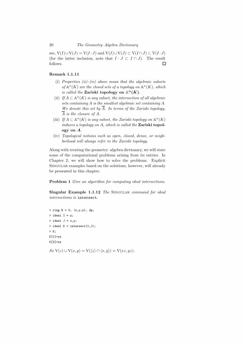
(v) The Kummer surface is an example of a hypersurface in
3–space:
Another example is Labs’ septic from Example 0.0.10.
(vi) The twisted cubic curve in A3(R) is obtained by inter-
secting the hypersurfaces V(y − x2) and V(xy − z):

1.1 Affine Algebraic Geometry 19
Taking vanishing loci defines a map V which sends sets of poly-
nomials to algebraic sets. We summarize the properties of V:
Proposition 1.1.10
(i) The map V reverses inclusions: If I ⊂ J are subsets of
K[x1, . . . , xn], then V(I) ⊃ V(J).
(ii) Affine space and the empty set are algebraic:
V(0) = An(K). V(1) = ∅.
(iii) The union of finitely many algebraic sets is algebraic: If
I1, . . . , Is are ideals of K[x1, . . . , xn], then
s⋃
k=1
V(Ik) = V(
s⋂
k=1
Ik).
(iv) The intersection of any family of algebraic sets is algebraic:
If {Iλ} is a family of ideals of K[x1, . . . , xn], then
⋂
λ
V(Iλ) = V
(∑
λ
Iλ
).
(v) A single point is algebraic: If a1, . . . , an ∈ K, then
V(x1 − a1, . . . , xn − an) = {(a1, . . . , an)}.
Proof All properties except (iii) are immediate from the defini-
tions. For (iii), by induction, it is enough to consider the case of
two ideals I, J ⊂ K[x1, . . . , xn]. Let I ·J be the ideal generated by
all elements of type f ·g, with f ∈ I and g ∈ J . Then, as is easy to
20 The Geometry–Algebra Dictionary
see, V(I)∪V(J) = V(I ·J) and V(I)∪V(J) ⊂ V(I ∩J) ⊂ V(I ·J)(for the latter inclusion, note that I · J ⊂ I ∩ J). The result
follows.
Remark 1.1.11
(i) Properties (ii)–(iv) above mean that the algebraic subsets
of An(K) are the closed sets of a topology on An(K), which
is called the Zariski topology on An(K).
(ii) If A ⊂ An(K) is any subset, the intersection of all algebraic
sets containing A is the smallest algebraic set containing A.
We denote this set by A. In terms of the Zariski topology,
A is the closure of A.
(iii) If A ⊂ An(K) is any subset, the Zariski topology on An(K)
induces a topology on A, which is called the Zariski topol-
ogy on A.
(iv) Topological notions such as open, closed, dense, or neigh-
borhood will always refer to the Zariski topology.
Along with treating the geometry–algebra dictionary, we will state
some of the computational problems arising from its entries. In
Chapter 2, we will show how to solve the problems. Explicit
Singular examples based on the solutions, however, will already
be presented in this chapter.
Problem 1 Give an algorithm for computing ideal intersections.
Singular Example 1.1.12 The Singular command for ideal
intersections is intersect.
> ring R = 0, (x,y,z), dp;
> ideal I = z;
> ideal J = x,y;
> ideal K = intersect(I,J);
> K;
K[1]=yz
K[2]=xz
So V(z) ∪ V(x, y) = V(〈z〉 ∩ 〈x, y〉) = V(xz, yz).
1.1 Affine Algebraic Geometry 21
Remark 1.1.13 The previous example is special in that we con-
sider ideals which are monomial. The intersection of monomial
ideals is obtained using a simple recipe: Given I = 〈m1, . . . ,mr〉and J = 〈n1, . . . , ns〉 in K[x1, . . . , xn], with monomial generators
mi and nj , the intersection I∩J is generated by the least common
multiples of the mi, nj. In particular, I ∩ J is monomial again.
Our next step in relating algebraic sets to ideals is to define some
kind of inverse to the map V:
Definition 1.1.14 If A ⊂ An(K) is any subset, the ideal
I(A) := {f ∈ K[x1, . . . , xn] | f(p) = 0 for all p ∈ A}
is called the vanishing ideal of A.
We summarize the properties of I and start relating I to V:
Proposition 1.1.15 Let R = K[x1, . . . , xn].
(i) I(∅) = R. If K is infinite, then I(An(K)) = 〈0〉.(ii) If A ⊂ B are subsets of An(K), then I(A) ⊃ I(B).
(iii) If A,B are subsets of An(K), then
I(A ∪B) = I(A) ∩ I(B).
(iv) For any subset A ⊂ An(K), we have
V(I(A)) = A.
(v) For any subset I ⊂ R, we have
I(V(I)) ⊃ I.
22 The Geometry–Algebra Dictionary
Proof Properties (ii), (iii), and (v) are easy consequences of the
definitions. The first statement in (i) is also clear. For the second
statement, let K be infinite, and let f ∈ K[x1, . . . , xn] be any
nonzero polynomial. We have to show that there is a point p ∈An(K) such that f(p) 6= 0. By our assumption on K, this is
clear for n = 1 since every nonzero polynomial in one variable has
at most finitely many zeros. If n > 1, write f in the form f =
a0(x1, . . . , xn−1) + a1(x1, . . . , xn−1)xn + . . .+ as(x1, . . . , xn−1)xsn.
Then ai is nonzero for at least one i. For such an i, we may
assume by induction that there is a point p ∈ An−1(K) such that
ai(p) 6= 0. Then f(p, xn) ∈ K[xn] is nonzero. Hence, there is
an element pn ∈ K such that f(p, pn) 6= 0. This proves (i). For
(iv), note that V(I(A)) ⊃ A. Let, now, V(J) be any algebraic set
containing A. Then f(p) = 0 for all f ∈ J and all p ∈ A. Hence,
J ⊂ I(A) and, thus, V(J) ⊃ V(I(A)), as desired.
Property (iv) above expresses V(I(A)) in terms of A. Likewise,
we wish to express I(V(I)) in terms of I . The following example
shows that the containment I(V(I)) ⊃ I may be strict.
Example 1.1.16 We have
I(V(xm)) = 〈x〉 for all m ≥ 1.
Definition 1.1.17 Let R be any ring, and let I ⊂ R be an ideal.
Then the set√I := {f ∈ R | fm ∈ I for some m ≥ 1}
is an ideal of R containing I. It is called the radical of I. If√I = I, then I is called a radical ideal.
Example 1.1.18 Consider a principal ideal in K[x1, . . . , xn]: If
f = fµ1
1 · · · fµss ∈ K[x1, . . . , xn]
is the decomposition of a polynomial into irreducible factors, then√〈f〉 = 〈f1 · · · fs〉.
The product f1 · · · fs, which is uniquely determined by f up to
multiplication by a constant, is called the square-free part of f .
If f = f1 · · · fs up to scalar, we say that f is square-free.
1.1 Affine Algebraic Geometry 23
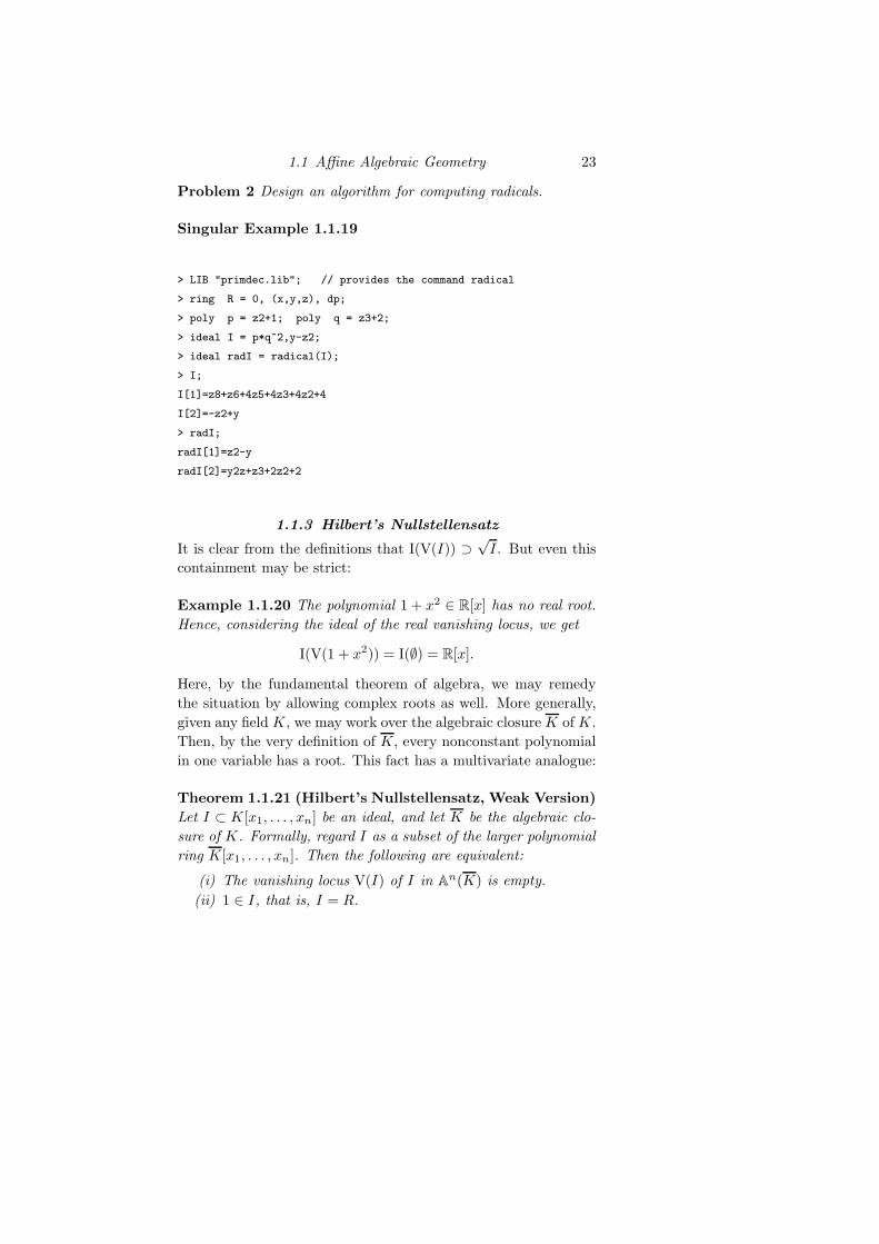
Problem 2 Design an algorithm for computing radicals.
Singular Example 1.1.19
> LIB "primdec.lib"; // provides the command radical
> ring R = 0, (x,y,z), dp;
> poly p = z2+1; poly q = z3+2;
> ideal I = p*q^2,y-z2;
> ideal radI = radical(I);
> I;
I[1]=z8+z6+4z5+4z3+4z2+4
I[2]=-z2+y
> radI;
radI[1]=z2-y
radI[2]=y2z+z3+2z2+2
1.1.3 Hilbert’s Nullstellensatz
It is clear from the definitions that I(V(I)) ⊃√I . But even this
containment may be strict:
Example 1.1.20 The polynomial 1 + x2 ∈ R[x] has no real root.
Hence, considering the ideal of the real vanishing locus, we get
I(V(1 + x2)) = I(∅) = R[x].
Here, by the fundamental theorem of algebra, we may remedy
the situation by allowing complex roots as well. More generally,
given any field K, we may work over the algebraic closure K of K.
Then, by the very definition of K, every nonconstant polynomial
in one variable has a root. This fact has a multivariate analogue:
Theorem 1.1.21 (Hilbert’s Nullstellensatz, Weak Version)
Let I ⊂ K[x1, . . . , xn] be an ideal, and let K be the algebraic clo-
sure of K. Formally, regard I as a subset of the larger polynomial
ring K[x1, . . . , xn]. Then the following are equivalent:
(i) The vanishing locus V(I) of I in An(K) is empty.
(ii) 1 ∈ I, that is, I = R.
24 The Geometry–Algebra Dictionary
The proof will be given in Section 1.1.8.
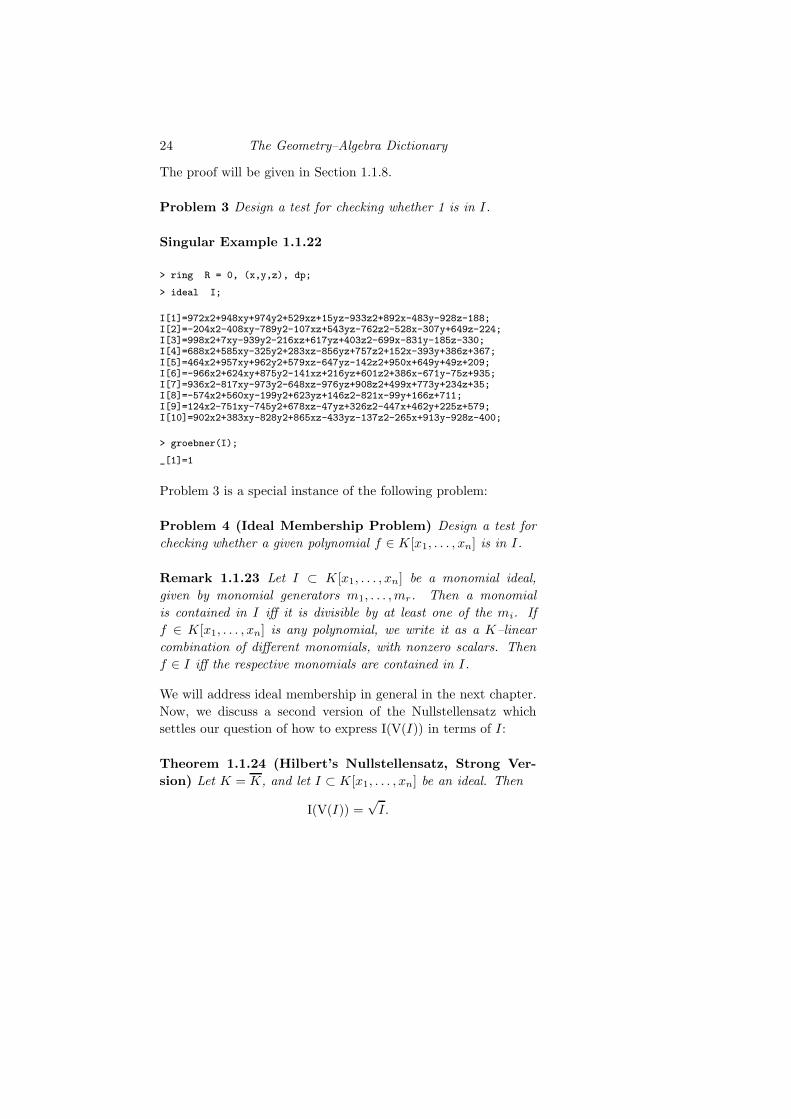
Problem 3 Design a test for checking whether 1 is in I.
Singular Example 1.1.22
> ring R = 0, (x,y,z), dp;
> ideal I;
I[1]=972x2+948xy+974y2+529xz+15yz-933z2+892x-483y-928z-188;I[2]=-204x2-408xy-789y2-107xz+543yz-762z2-528x-307y+649z-224;I[3]=998x2+7xy-939y2-216xz+617yz+403z2-699x-831y-185z-330;I[4]=688x2+585xy-325y2+283xz-856yz+757z2+152x-393y+386z+367;I[5]=464x2+957xy+962y2+579xz-647yz-142z2+950x+649y+49z+209;I[6]=-966x2+624xy+875y2-141xz+216yz+601z2+386x-671y-75z+935;I[7]=936x2-817xy-973y2-648xz-976yz+908z2+499x+773y+234z+35;I[8]=-574x2+560xy-199y2+623yz+146z2-821x-99y+166z+711;I[9]=124x2-751xy-745y2+678xz-47yz+326z2-447x+462y+225z+579;I[10]=902x2+383xy-828y2+865xz-433yz-137z2-265x+913y-928z-400;
> groebner(I);
_[1]=1
Problem 3 is a special instance of the following problem:
Problem 4 (Ideal Membership Problem) Design a test for
checking whether a given polynomial f ∈ K[x1, . . . , xn] is in I.
Remark 1.1.23 Let I ⊂ K[x1, . . . , xn] be a monomial ideal,
given by monomial generators m1, . . . ,mr. Then a monomial
is contained in I iff it is divisible by at least one of the mi. If
f ∈ K[x1, . . . , xn] is any polynomial, we write it as a K–linear
combination of different monomials, with nonzero scalars. Then
f ∈ I iff the respective monomials are contained in I.
We will address ideal membership in general in the next chapter.
Now, we discuss a second version of the Nullstellensatz which
settles our question of how to express I(V(I)) in terms of I :
Theorem 1.1.24 (Hilbert’s Nullstellensatz, Strong Ver-
sion) Let K = K, and let I ⊂ K[x1, . . . , xn] be an ideal. Then
I(V(I)) =√I.
1.1 Affine Algebraic Geometry 25
Proof As already pointed out earlier,√I ⊂ I(V(I)). The opposite
inclusion can be reduced to the weak version of the Nullstellensatz.
We briefly sketch the main idea: Let f ∈ I(V(I)), and let f1, . . . , frbe generators for I . Then f vanishes on V(I), and we have to show
that fm = g1f1+ . . .+ grfr for some m ≥ 1 and some g1, . . . , gr ∈K[x1, . . . , xn]. This follows by using the trick of Rabinowitch:
Consider the ideal
J := 〈f1, . . . , fr, yf − 1〉 ⊂ K[x1, . . . , xn, y],
where y is an extra variable. Show that V(J) ⊂ An+1(K) is empty.
Then apply the weak version of the Nullstellensatz to conclude
that 1 ∈ J . To get the result, represent 1 as a K[x1, . . . , xn, y]–
linear combination of f1, . . . , fr, yf − 1.
Corollary 1.1.25 If K = K, then I and V define a one–to–one
correspondence{algebraic subsets of An(K)}
I ↑ ↓ V
{radical ideals of K[x1, . . . , xn]}.The trick of Rabinowitch allows us to solve the following problem:
Corollary 1.1.26 (Radical Membership) Let K be any field,
let I ⊂ K[x1, . . . , xn] be an ideal, and let f ∈ K[x1, . . . , xn]. Then:
f ∈√I ⇐⇒ 1 ∈ J := 〈I, yf − 1〉 ⊂ K[x1, . . . , xn, y],
where y is an extra variable.
Based on the Nullstellensatz, we can express geometric properties
in terms of ideals. Here is a first example of how this works:
Proposition 1.1.27 Let K be any field, and let I ⊂ K[x1, . . . , xn]
be an ideal. The following are equivalent:
(i) The vanishing locus V(I) of I in An(K) is finite (or empty).
(ii) For each i, 1 ≤ i ≤ n, we have I ∩K[xi] ) 〈0〉.
Problem 5 Design a test for checking whether (ii) holds.
What we ask here is reminiscent of what we did in Example 0.0.7:
Checking (ii) means to eliminate all but one of the variables.
26 The Geometry–Algebra Dictionary
Example 1.1.28 Taking the symmetry of the generators into ac-
count, the computation in Example 0.0.7 shows that the ideal
I = 〈x+ y+ z− 1, x2 + y2 + z2 − 1, x3 + y3 + z3 − 1〉 ⊂ Q[x, y, z]
contains the polynomials
z3 − z2, y3 − y2, x3 − x2.
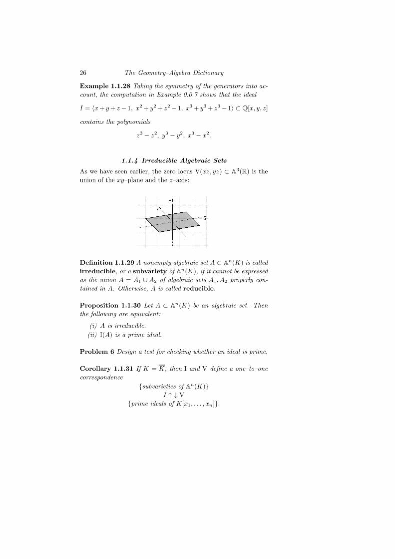
1.1.4 Irreducible Algebraic Sets
As we have seen earlier, the zero locus V(xz, yz) ⊂ A3(R) is the
union of the xy–plane and the z–axis:
Definition 1.1.29 A nonempty algebraic set A ⊂ An(K) is called
irreducible, or a subvariety of An(K), if it cannot be expressed
as the union A = A1 ∪ A2 of algebraic sets A1, A2 properly con-
tained in A. Otherwise, A is called reducible.
Proposition 1.1.30 Let A ⊂ An(K) be an algebraic set. Then
the following are equivalent:
(i) A is irreducible.
(ii) I(A) is a prime ideal.
Problem 6 Design a test for checking whether an ideal is prime.
Corollary 1.1.31 If K = K, then I and V define a one–to–one
correspondence
{subvarieties of An(K)}I ↑ ↓ V
{prime ideals of K[x1, . . . , xn]}.
1.1 Affine Algebraic Geometry 27
Proposition 1.1.32 If K = K, then I and V define a one–to–one
correspondence{points of An(K)}
I ↑ ↓ V
{maximal ideals of K[x1, . . . , xn]}.Here is the main result in this section:
Theorem 1.1.33 Every nonempty algebraic set A ⊂ An(K) can
be expressed as a finite union
A = V1 ∪ · · · ∪ Vs
of subvarieties Vi. This decomposition can be chosen to be mini-
mal in the sense that Vi 6⊃ Vj for i 6= j. The Vi are, then, uniquely
determined and are called the irreducible components of A.
Proof The main idea of the proof is to use Noetherian induc-
tion: Assuming that there is an algebraic set A ⊂ An(K) which
cannot be written as a finite union of irreducible subsets, we get
an infinite descending chain of subvarieties Vi of A:
A ⊃ V1 ) V2 ) . . .
This contradicts the ascending condition in the polynomial ring
since taking vanishing ideals is inclusion reversing.
Problem 7 Give an algorithm to find the irreducible components.
The algebraic concept of primary decomposition gives an answer
to both Problems 7 and 6 (see Section 2.3). If K is a subfield
of C, and if all irreducible components in An(C) are points (that
is, we face a system of polynomial equations with just finitely
many complex solutions), we may find the solutions via trian-
gular decomposition. This method combines Grobner bases with
univariate numerical solving . See [Decker and Lossen (2006)].
Singular Example 1.1.34
> ring S = 0, (x,y,z), lp;
> ideal I = x2+y+z-1, x+y2+z-1, x+y+z2-1;
> LIB "solve.lib";
28 The Geometry–Algebra Dictionary
> def R = solve(I,6); // creates a new ring in which the solutions
. // are defined; 6 is the desired precision
setring R; SOL;
//-> [1]: [2]: [3]: [4]: [5]:
//-> [1]: [1]: [1]: [1]: [1]:
//-> 0.414214 0 -2.414214 1 0
//-> [2]: [2]: [2]: [2]: [2]:
//-> 0.414214 0 -2.414214 0 1
//-> [3]: [3]: [3]: [3]: [3]:
//-> 0.414214 1 -2.414214 0 0
In this simple example, the solutions can also be read off from a
lexicographic Grobner basis as in Example 0.0.7:
> groebner(I);
//-> _[1]=z6-4z4+4z3-z2 _[2]=2yz2+z4-z2
//-> _[3]=y2-y-z2+z _[4]=x+y+z2-1
1.1.5 Removing Algebraic Sets
The set theoretic difference of two algebraic sets needs not be an
algebraic set:
Example 1.1.35 Consider again the union of of the xy–plane
and the z–axis in A3(R):
Removing the plane, the residual set is the punctured z–axis, which
is not defined by polynomial equations. Indeed, if a polynomial
f ∈ R[x, y, z] vanishes on the z–axis except possibly at the origin
o, then the univariate polynomial g(t) := f(0, 0, t) has infinitely
many roots since R is infinite. Hence, g = 0 (see the proof of
Proposition 1.1.15), so that f vanishes at o, too.
1.1 Affine Algebraic Geometry 29
In what follows, we explain how to find polynomial equations for
the Zariski closure of the difference of two algebraic sets, that is,
for the smallest algebraic set containing the difference. We need
the following notation:
Definition 1.1.36 If I, J are two ideals of a ring R, the set
I : J := {f ∈ R | fg ∈ I for all g ∈ J}
is an ideal of R containing I. It is called the ideal quotient of
I by J .
Definition 1.1.37 If I, J are two ideals of a ring R, the set
I : J∞ := {f ∈ R | fJm ⊂ I for some m ≥ 1} =∞⋃
m=1
(I : Jm)
is an ideal of R containing I. It is called the saturation of I with
respect to J .
Theorem 1.1.38 Let I, J be ideals of K[x1, . . . , xn]. Then, con-
sidering vanishing loci and the Zariski closure in An(K), we have
V(I) \V(J) = V(I : J∞) ⊂ An(K).
If I is a radical ideal, then
V(I) \V(J) = V(I : J) ⊂ An(K).
The proof of the theorem is somewhat technical and makes use of
of primary decomposition (see [Decker and Schreyer (to appear)]).
Problem 8 Design algorithms for computing ideal quotients and
saturation.
Since the polynomial ringK[x1, . . . , xn] is Noetherian by Hilbert’s
basis theorem, and since I : Jm = (I : Jm−1) : J for any two ideals
I, J ⊂ K[x1, . . . , xn], the computation of the saturation
I : J∞ =∞⋃
m=1
(I : Jm)
30 The Geometry–Algebra Dictionary
just means to iterate the computation of ideal quotients. Indeed,
the ascending chain
I : J ⊂ I : J2 ⊂ · · · ⊂ I : Jm ⊂ . . .
is eventually stationary.
Singular Example 1.1.39 To simplify the output, we work over
the field with 2 elements:
> ring R = 2, (x,y,z), dp;
> poly F = x5+y5+(x-y)^2*xyz;
> ideal J = jacob(F);
> J;
//-> J[1]=x4+x2yz+y3z J[2]=y4+x3z+xy2z J[3]=x3y+xy3
> maxideal(2);
//-> _[1]=z2 _[2]=yz _[3]=y2 _[4]=xz _[5]=xy _[6]=x2
> ideal K = quotient(J,maxideal(2));
> K;
//-> K[1]=y4+x3z+xy2z K[2]=x3y+xy3 K[3]=x4+x2yz+y3z
//-> K[4]=x3z2+x2yz2+xy2z2+y3z2 K[5]=x2y2z+x2yz2+y3z2
//-> K[6]=x2y3
> K = quotient(K,maxideal(2)); K;
K[1]=x3+x2y+xy2+y3
K[2]=y4+x2yz+y3z
K[3]=x2y2+y4
> K = quotient(K,maxideal(2)); K;
K[1]=x3+x2y+xy2+y3
K[2]=y4+x2yz+y3z
K[3]=x2y2+y4
The Singular library elim.lib provides the command sat for
saturation:
> LIB "elim.lib";
> int p = printlevel;
> printlevel = 2; // print more information while computing
> sat(J,maxideal(2));
// compute quotient 1
// compute quotient 2
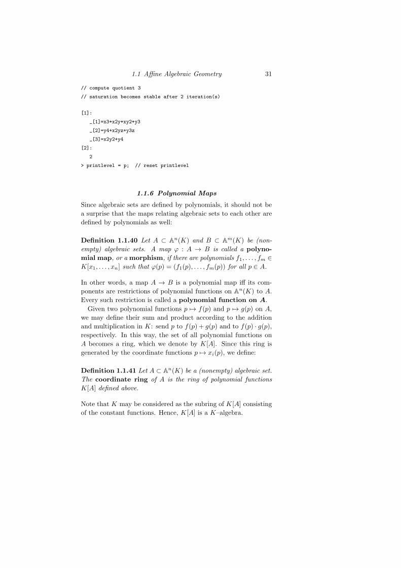
1.1 Affine Algebraic Geometry 31
// compute quotient 3
// saturation becomes stable after 2 iteration(s)
[1]:
_[1]=x3+x2y+xy2+y3
_[2]=y4+x2yz+y3z
_[3]=x2y2+y4
[2]:
2
> printlevel = p; // reset printlevel
1.1.6 Polynomial Maps
Since algebraic sets are defined by polynomials, it should not be
a surprise that the maps relating algebraic sets to each other are
defined by polynomials as well:
Definition 1.1.40 Let A ⊂ An(K) and B ⊂ Am(K) be (non-
empty) algebraic sets. A map ϕ : A → B is called a polyno-
mial map, or a morphism, if there are polynomials f1, . . . , fm ∈K[x1, . . . , xn] such that ϕ(p) = (f1(p), . . . , fm(p)) for all p ∈ A.
In other words, a map A → B is a polynomial map iff its com-
ponents are restrictions of polynomial functions on An(K) to A.
Every such restriction is called a polynomial function on A.
Given two polynomial functions p 7→ f(p) and p 7→ g(p) on A,
we may define their sum and product according to the addition
and multiplication in K: send p to f(p) + g(p) and to f(p) · g(p),respectively. In this way, the set of all polynomial functions on
A becomes a ring, which we denote by K[A]. Since this ring is
generated by the coordinate functions p 7→ xi(p), we define:
Definition 1.1.41 Let A ⊂ An(K) be a (nonempty) algebraic set.
The coordinate ring of A is the ring of polynomial functions
K[A] defined above.
Note that K may be considered as the subring of K[A] consisting
of the constant functions. Hence, K[A] is a K–algebra.
32 The Geometry–Algebra Dictionary
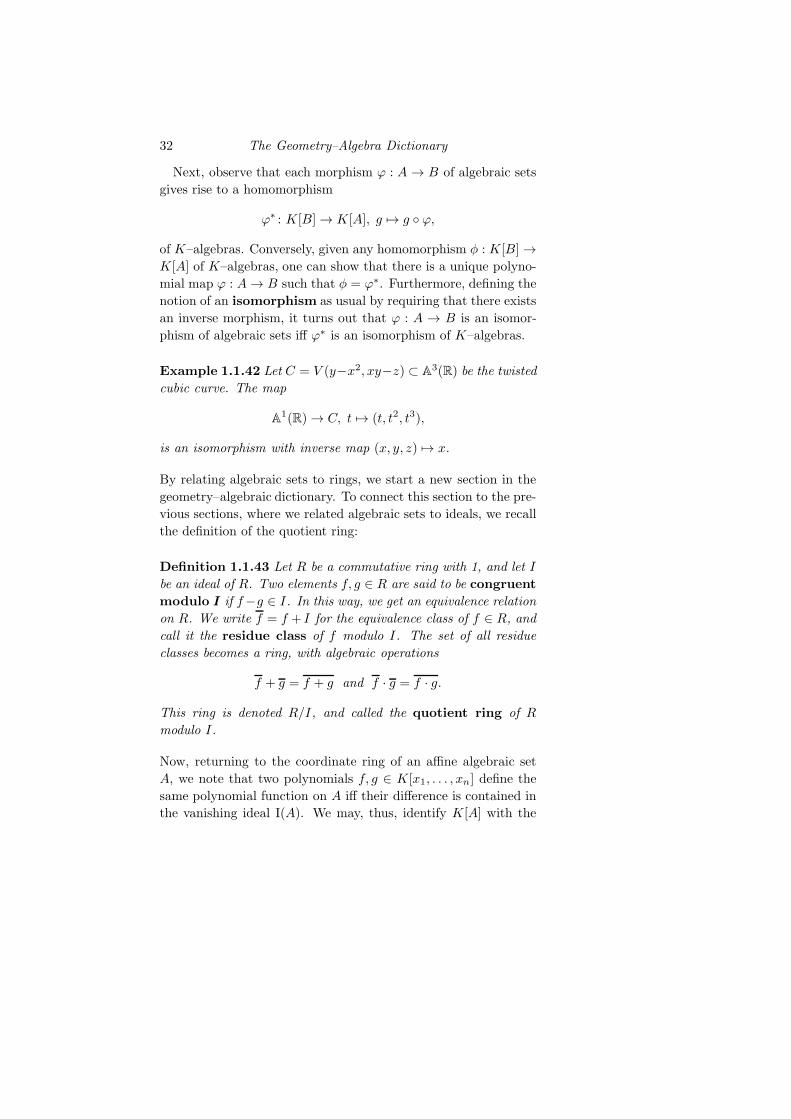
Next, observe that each morphism ϕ : A → B of algebraic sets
gives rise to a homomorphism
ϕ∗ : K[B] → K[A], g 7→ g ◦ ϕ,
of K–algebras. Conversely, given any homomorphism φ : K[B] →K[A] of K–algebras, one can show that there is a unique polyno-
mial map ϕ : A → B such that φ = ϕ∗. Furthermore, defining the
notion of an isomorphism as usual by requiring that there exists
an inverse morphism, it turns out that ϕ : A → B is an isomor-
phism of algebraic sets iff ϕ∗ is an isomorphism of K–algebras.
Example 1.1.42 Let C = V (y−x2, xy−z) ⊂ A3(R) be the twistedcubic curve. The map
A1(R) → C, t 7→ (t, t2, t3),
is an isomorphism with inverse map (x, y, z) 7→ x.
By relating algebraic sets to rings, we start a new section in the
geometry–algebraic dictionary. To connect this section to the pre-
vious sections, where we related algebraic sets to ideals, we recall
the definition of the quotient ring:
Definition 1.1.43 Let R be a commutative ring with 1, and let I
be an ideal of R. Two elements f, g ∈ R are said to be congruent
modulo I if f−g ∈ I. In this way, we get an equivalence relation
on R. We write f = f + I for the equivalence class of f ∈ R, and
call it the residue class of f modulo I. The set of all residue
classes becomes a ring, with algebraic operations
f + g = f + g and f · g = f · g.
This ring is denoted R/I, and called the quotient ring of R
modulo I.
Now, returning to the coordinate ring of an affine algebraic set
A, we note that two polynomials f, g ∈ K[x1, . . . , xn] define the
same polynomial function on A iff their difference is contained in
the vanishing ideal I(A). We may, thus, identify K[A] with the
1.1 Affine Algebraic Geometry 33
quotient ring K[x1, . . . , xn]/I(A), and translate geometric proper-
ties expressed in terms of I(A) into properties expressed in terms
of K[A]. For example:
• A is irreducible ⇐⇒ I(A) is prime ⇐⇒ K[x1, . . . , xn]/I(A) is
an integral domain.
For another example, let I ( K[x1, . . . , xn] be any proper ideal.
Then K[x1, . . . , xn]/I contains K as a subring, so that R/I is
a K–vector space. This allows us, as one can show, to rewrite
Proposition 1.1.27 as follows:
• The vanishing locus V(I) of I in An(K) is finite (or empty) ⇐⇒K[x1, . . . , xn]/I is a K–vector space of finite dimension.
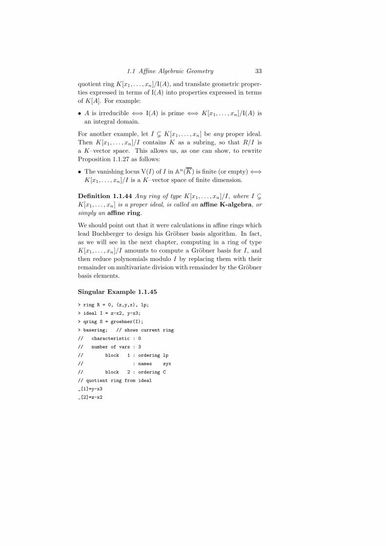
Definition 1.1.44 Any ring of type K[x1, . . . , xn]/I, where I (K[x1, . . . , xn] is a proper ideal, is called an affine K-algebra, or
simply an affine ring.
We should point out that it were calculations in affine rings which
lead Buchberger to design his Grobner basis algorithm. In fact,
as we will see in the next chapter, computing in a ring of type
K[x1, . . . , xn]/I amounts to compute a Grobner basis for I , and
then reduce polynomials modulo I by replacing them with their
remainder on multivariate division with remainder by the Grobner
basis elements.
Singular Example 1.1.45
> ring R = 0, (z,y,x), lp;
> ideal I = z-x2, y-x3;
> qring S = groebner(I);
> basering; // shows current ring
// characteristic : 0
// number of vars : 3
// block 1 : ordering lp
// : names zyx
// block 2 : ordering C
// quotient ring from ideal
_[1]=y-x3
_[2]=z-x2
34 The Geometry–Algebra Dictionary
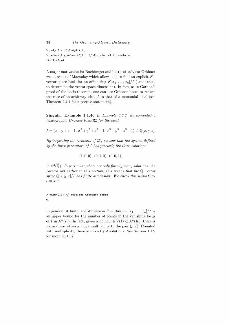
> poly f = x3z2-4y4z+x4;
> reduce(f,groebner(0)); // division with remainder
-4x14+x7+x4
A major motivation for Buchberger and his thesis advisor Grobner
was a result of Macaulay which allows one to find an explicit K–
vector space basis for an affine ring K[x1, . . . , xn]/I ( and, thus,
to determine the vector space dimension). In fact, as in Gordan’s
proof of the basis theorem, one can use Grobner bases to reduce
the case of an arbitrary ideal I to that of a monomial ideal (see
Theorem 2.4.1 for a precise statement).
Singular Example 1.1.46 In Example 0.0.7, we computed a
lexicographic Grobner basis GI for the ideal
I = 〈x+ y+ z− 1, x2 + y2+ z2− 1, x3 + y3+ z3− 1〉 ⊂ Q[x, y, z].
By inspecting the elements of GI, we saw that the system defined
by the three generators of I has precisely the three solutions
(1, 0, 0), (0, 1, 0), (0, 0, 1).
in A3(Q). In particular, there are only finitely many solutions. As
pointed out earlier in this section, this means that the Q–vector
space Q[x, y, z]/I has finite dimension. We check this using Sin-
gular:
> vdim(GI); // requires Groebner basis
6
In general, if finite, the dimension d = dimK K[x1, . . . , xn]/I is
an upper bound for the number of points in the vanishing locus
of I in An(K). In fact, given a point p ∈ V(I) ⊂ An(K), there is
natural way of assigning a multiplicity to the pair (p, I). Counted
with multiplicity, there are exactly d solutions. See Section 1.1.9
for more on this.
1.1 Affine Algebraic Geometry 35
1.1.7 The Geometry of Elimination
The image of an affine algebraic set under a morphism needs not
be an algebraic set†‡:
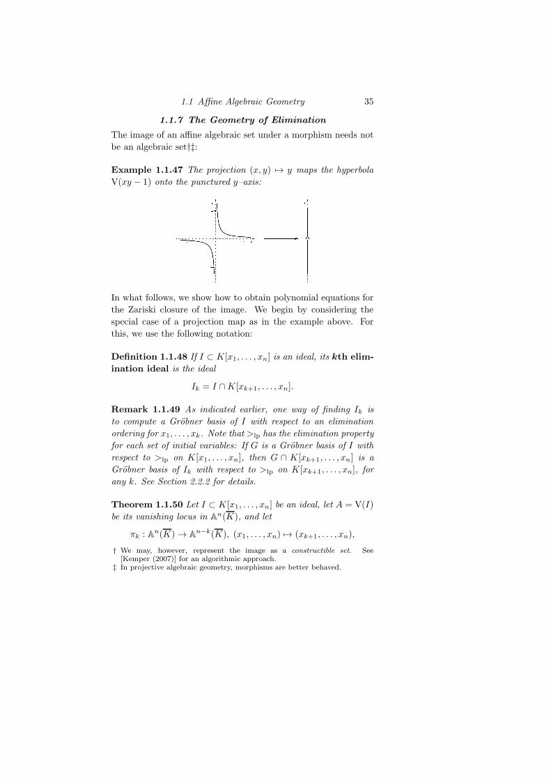
Example 1.1.47 The projection (x, y) 7→ y maps the hyperbola
V(xy − 1) onto the punctured y–axis:
In what follows, we show how to obtain polynomial equations for
the Zariski closure of the image. We begin by considering the
special case of a projection map as in the example above. For
this, we use the following notation:
Definition 1.1.48 If I ⊂ K[x1, . . . , xn] is an ideal, its kth elim-
ination ideal is the ideal
Ik = I ∩K[xk+1, . . . , xn].
Remark 1.1.49 As indicated earlier, one way of finding Ik is
to compute a Grobner basis of I with respect to an elimination
ordering for x1, . . . , xk. Note that >lp has the elimination property
for each set of initial variables: If G is a Grobner basis of I with
respect to >lp on K[x1, . . . , xn], then G ∩ K[xk+1, . . . , xn] is a
Grobner basis of Ik with respect to >lp on K[xk+1, . . . , xn], for
any k. See Section 2.2.2 for details.
Theorem 1.1.50 Let I ⊂ K[x1, . . . , xn] be an ideal, let A = V(I)
be its vanishing locus in An(K), and let
πk : An(K) → An−k(K), (x1, . . . , xn) 7→ (xk+1, . . . , xn),
† We may, however, represent the image as a constructible set. See[Kemper (2007)] for an algorithmic approach.
‡ In projective algebraic geometry, morphisms are better behaved.
36 The Geometry–Algebra Dictionary
be projection onto the last n− k variables. Then
πk(A) = V(Ik) ⊂ An−k(K).
Proof As we will explain in Section 2.5, the ideal generated by
Ik in the polynomial ring K[xk+1, . . . , , xn] is the first elimination
ideal of the ideal generated by I inK[x1, . . . , , xn]. We may, hence,
suppose that K = K. The theorem is, then, an easy consequence
of the Nullstellensatz. We leave the details to the reader.
In what follows, we write x = {x1, . . . , xn} and y = {y1, . . . , ym},and consider the xi and yj as the coordinate functions on An(K)
and Am(K), respectively. Furthermore, given an ideal I ⊂ K[x],
we write I K[x, y] for the ideal of K[x, y] generated by I .
Corollary 1.1.51 Let I ⊂ K[x] be an ideal, let A = V(I) ⊂An(K), and let
ϕ : A → Am(K), p 7→ (f1(p), . . . , fm(p)),
be a morphism, given by polynomials f1, . . . , fm ∈ K[x]. Let J be
the ideal
J = I K[x, y] + 〈f1 − y1, . . . , fm − ym〉 ⊂ K[x, y].
Then
ϕ(A) = V(J ∩K[y]) ⊂ Am(K).
That is, the vanishing locus of the elimination ideal J ∩ K[y] in
Am(K) is the Zariski closure of ϕ(A).
Proof The result follows from Theorem 1.1.50 since the ideal J
describes the graph of ϕ in An+m(K).
Remark 1.1.52 Algebraically, as we will see in Section 2.2.6, J
is the kernel of the ring homomorphism
φ : K[y1, . . . , ym] → S = K[x1, . . . , xn]/I, yi 7→ f i = fi + I.
Under an additional assumption, the statement of Corollary 1.1.51
holds in the geometric setting over the original field K:
1.1 Affine Algebraic Geometry 37
Corollary 1.1.53 Let I, f1, . . . , fm, and J be as in Corollary
1.1.51. let A = V(I) ⊂ An(K), and let
ϕ : A → Am(K), p 7→ (f1(p), . . . , fm(p)),
be the morphism defined by f1, . . . , fm. Suppose that the vanishing
locus of I in An(K) is the Zariski closure of A in An(K). Then
ϕ(A) = V(J ∩K[y]) ⊂ Am(K).
If K is infinite, then the condition on A in Corollary 1.1.53 is ful-
filled for A = An(K). It, hence, applies in the following Example.
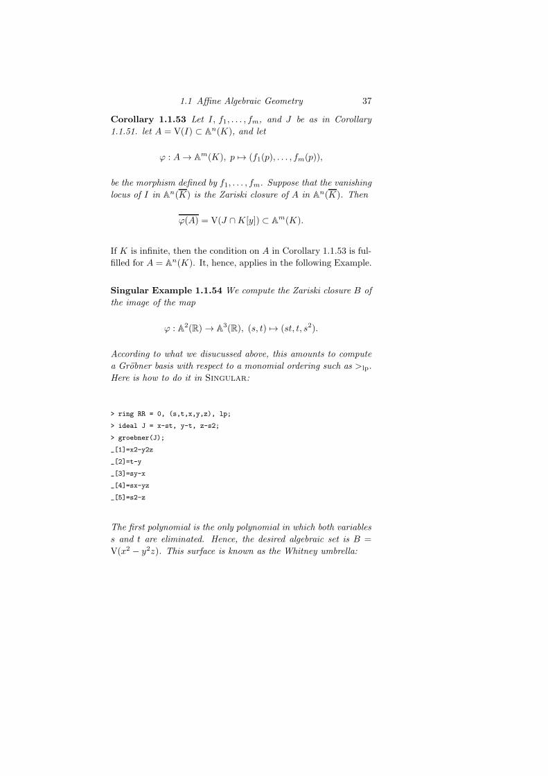
Singular Example 1.1.54 We compute the Zariski closure B of
the image of the map
ϕ : A2(R) → A3(R), (s, t) 7→ (st, t, s2).
According to what we disucussed above, this amounts to compute
a Grobner basis with respect to a monomial ordering such as >lp.
Here is how to do it in Singular:
> ring RR = 0, (s,t,x,y,z), lp;
> ideal J = x-st, y-t, z-s2;
> groebner(J);
_[1]=x2-y2z
_[2]=t-y
_[3]=sy-x
_[4]=sx-yz
_[5]=s2-z
The first polynomial is the only polynomial in which both variables
s and t are eliminated. Hence, the desired algebraic set is B =
V(x2 − y2z). This surface is known as the Whitney umbrella:
38 The Geometry–Algebra Dictionary
V(x2 − y2z)
Alternatively, we may use the built–in Singular command eliminate
to compute the equation of the Whitney umbrella:
> ideal K = eliminate(J,st);
K;
K[1]=y2z-x2
> ring R = 0, (x,y,z), dp;
> ideal K = imap(RR,K);
K;
K[1]=y2z-x2
The map ϕ considered above is an example of what we will call a
polynomial parametrization:
Definition 1.1.55 Let B ⊂ Am(K) be algebraic. A polynomial
parametrization of B is a morphism ϕ : An(K) → Am(K) such
that B is the Zariski closure of the image of ϕ.
Instead of just considering polynomial maps, we are more gener-
ally interested in rational maps, that is, in maps of type
t = (t1, . . . , tn) 7→ (g1(t)
h1(t), . . . ,
gm(t)
hm(t)),
with polynomials gi, hi ∈ K[x1, . . . , xn] (see Example 1.1.9, (iv)).
Note that such a map may not be defined on all of An(K) because
of the denominators. We have, however, a well–defined map
ϕ : An(K) \V(h1 · · ·hm) → Am(K), t 7→ (g1(t)
h1(t), . . . ,
gm(t)
hm(t)).
1.1 Affine Algebraic Geometry 39
Our next result will allow us to compute the Zariski closure of the
image of such a map:
Proposition 1.1.56 Let K be infinite. Given g1, . . . , gm and
h1, . . . , hm in K[x] = K[x1, . . . , xn], consider the map
ϕ : U → Am(K), t 7→ (g1(t)
h1(t), . . . ,
gm(t)
hm(t)),
where U = An(K) \V(h1 · · ·hm). Let J be the ideal
J = 〈h1x1 − g1, . . . , hmxm − gm, 1− h1 · · ·hm · w〉 ⊂ K[w, x, y],
where y stands for the coordinate functions y1, . . . , ym on Am(K),
and where w is an extra variable. Then
ϕ(U) = V(J ∩K[y]) ⊂ Am(K).
Singular Example 1.1.57 We demonstrate the use of Proposi-
tion 1.1.56 in an example:
> ring RR = 0, (w,t,x,y), dp;
> poly g1 = 2t; poly h1 = t2+1;
> poly g2 = t2-1; poly h2 = t2+1;
> ideal J = h1*x-g1, h2*y-g2, 1-h1*h2*w;
> ideal K = eliminate(J,wt);
> K;
K[1]=x2+y2-1
> ring R = 0, (x,y), dp;
> ideal K = imap(RR,K);
> K;
K[1]=x2+y2-1
The resulting equation defines the unit circle. Note that the circle
does not admit a polynomial parametrization.
Definition 1.1.58 Let B ⊂ Am(K) be algebraic. A rational
parametrization of B is a map ϕ as in Proposition 1.1.56 such
that B is the Zariski closure of the image of ϕ.