1

THE USE OF A COMBINED PORTABLE X RAY FLUORESCENCE AND 1

MULTIVARIATE STATISTICAL METHODS TO ASSESS A VALIDATED 2

MACROSCOPIC ROCK SAMPLES CLASSIFICATION IN AN ORE 3

EXPLORATION SURVEY. 4

5

Figueroa Cisterna, J. (a); Bagur González, M.G. (b,c) ( ); Morales Ruano, S. (a,c); 6 Carrillo Rosúa, J.C. (c,d) and Martín Peinado, F.(e) 7

8

(a) Department of Mineralogy and Petrology, Faculty of Sciences, Avda. Fuentenueva s/n, 9

University of Granada, 18071, Granada, Spain 10

11

(b) Department of Analytical Chemistry, Faculty of Sciences, Avda. Fuentenueva s/n, 12

University of Granada, 18071, Granada, Spain. 13

14

(c) Instituto Andaluz de Ciencias de la Tierra (University of Granada-CSIC), Faculty of 15

Sciences, Avda. Fuentenueva s/n, University of Granada, 18071, Granada, Spain. 16

17

(d) Department of Didactics of Experimental Sciences. Faculty of Education Sciences, 18

Campus de Cartuja s/n, University of Granada, 18071, Granada, Spain. 19

20

(e) Department of Soil Science, Faculty of Sciences, Avda. Fuentenueva, University of 21

Granada, 18071, Granada, Spain. 22

23

Keywords: Portable X Ray Fluorescence Analyzer (P-XRF), Box-Cox Transformation, 24

Pattern Recognition Techniques, Ore Exploration, Cu-(Ag) Deposits. 25

26

( ) Corresponding author: Phone: +34958243327; Fax: +34958243328

e-mail: mgbagur@ugr.es

27

Postprint versión.  Original paper: Figueroa‐Cisterna, J., Bagur‐González, M. G., Morales‐Ruano, S., Carrillo‐Rosúa, J., & Martín‐Peinado, F. (2011). The use of a combined portable X ray fluorescence and multivariate statistical methods to assess a validated macroscopic rock samples classification in an ore exploration survey. Talanta, 85(5), 2307‐2315. doi:10.1016/j.talanta.2011.07.034 

2

Abstract 1

2

The combination of “ex-situ” portable X Ray Fluorescence with unsupervised and 3

supervised pattern recognition techniques such as hierarchical cluster analysis, principal 4

components analysis, factor analysis and linear discriminant analysis have been applied 5

to rock samples, in order to validate a “in situ” macroscopic rock samples classification 6

of samples collected in the Boris Angelo mining area (Central Chile), during a drill-hole 7

survey carried out to evaluate the economic potential of this Cu deposit. The analysed 8

elements were Ca, Cu, Fe, K, Mn, Pb, Rb, Sr, Ti and Zn. The statistical treatment of the 9

geological data has been arisen from the application of the Box-Cox transformation 10

used to transform the data set in normal form to minimize the non-normal distribution 11

of the data. From the statistical results obtained it can be concluded that the 12

macroscopic classification applied to the transformed data permits at least, to 13

distinguish quite well in relation to two of the rock classes defined (70.5 % correctly 14

classified (p< 0.05)) as well as for four of the five alteration types defined “in situ” 15

(75% of the total samples). 16

17

3

1. Introduction 1

2

The extraction of metals from the earth crust initially requires the identification 3

of the areas in which they have anomalous concentration in relation to the host rock of 4

the ore mineralization and, in general sense, to the background in the mining zone. In 5

this sense, the geological characterization of the potential host rocks of ore 6

mineralization is crucial and must be the preliminary objective in any exploration 7

survey. 8

9

In relation with this fact, two fundamental stages must be covered, the 10

establishment of the geological cartography and the drill-hole survey. The former 11

because permits the knowledge of the main geological features (lithologies, structures, 12

mineralization evidences, etc.) and the later because gives an invaluable set of data over 13

the geology under the surface. From the study of the information obtained in these 14

stages it is possible to get a three dimensional idea about the existing rocks and their 15

characteristics. Thus recognition and classification of the different rock types, as well as 16

its alteration pattern, play an important role which could be critic in the selection of the 17

areas that could be adequate to explore host ore bodies with economic interest. 18

19

During the initial field campaign necessary in order to obtain the data, a lot of 20

samples are generates. In this sense, they must be classified attending criteria closely 21

related to the type of deposits to be exploited, e.g. type of lithologies, hydrothermal 22

alteration patterns among others. In the most of the cases these criteria are applied “in 23

situ” in remote areas without confirmatory analytical information from a laboratory, 24

and, in the best of the cases, using basic equipment like a magnifying glass or some safe 25

and easily portable chemical reagent. In this way, it could be helpfully to dispose of 26

qualimetric tools that could validate this macroscopic rock samples classification in 27

order to facilitate and accelerated the remained work necessary to determine the 28

goodness of the ulterior mining exploration of the zone investigated. 29

30

Bearing in mind these reasons, the use of analytical techniques as portable X-ray 31

fluorescence (P-XRF) combined with statistical pattern recognition techniques can be 32

offered as an adequate tool in order to obtain a feasible model that could permits the 33

4

assessment of a validated macroscopic rocks samples classification in an ore exploration 1

survey. 2

3

Up to the present day, the use of field portable X-ray fluorescence (P-XRF) 4

analysers [1-5] has been demonstrated be adequate in order to solve questions related 5

with a great variety of deals, e.g. for the assessment of the composition of painting 6

materials in order to offer information about their conservation and/or restoration 7

procedures [6,7], for archaeological studies [8,9], for the screening and assessment 8

studies about metalloids and/or heavy metals in contaminated or potentially 9

contaminated areas [3,4,10-14], FDA regulated products [15], or metal contents in 10

waters [16], among others. On the other hand, the relatively low cost of these devices 11

permits the possibility of their use in lab for routine analysis in quality control 12

assessments. 13

14

In parallel, it has been demonstrated that the use of unsupervised and supervised 15

pattern recognition techniques permits to extract reliable information from analytical 16

parameters for exploratory assessment of geological sets [17-19], mainly due to they 17

allow (a) to verify associations among variables, (b) to group or to cluster samples with 18

respect to comparable chemical or geological descriptors, and (c) to search multivariate 19

data classification on the basis of known class membership of those objects. 20

21

Nowadays, copper is one of the most demanded materials on the metal market 22

showing a growing demand perspective at the present such as the future. Together with 23

this growing demand, the exploration of this metal has been widespread for the entire 24

world to satisfy the copper supply. In this context, Chile is the first copper-producing 25

country holding a 36% of the world production of this metal. 26

27

Boris Angelo Cu-(Ag) deposit is located in the “stratabound Cu-(Ag) belt” [20] 28

in the Costal Cordillera, Central Chile. It corresponds to practically unknown deposit in 29

this belt, thus the study carried out in the area can be considered as a typical case study 30

of an exploration survey of a copper deposit. In this paper, a normalized data matrix 31

obtained from P-XRF measurements of rocks samples from a “preliminary ore 32

exploratory survey” has been subjected to different pattern recognition techniques in 33

5

order to confirm the rock classification parameters of samples taken during the drill-1

hole survey made in the Boris Angelo area. 2

3

2. Material and Methods 4

5

2.1. Studied area and macroscopic classification defined 6

7

The Boris Angelo Cu-(Ag) deposit is located in the easternmost Coastal 8

Cordillera, in Central Chile, between 32º30’ S and 70º40’ W (Fig. 1). It is part of the 9

Cretaceous stratabound Cu-(Ag) deposits belt, which are also known as “Chilean 10

Manto-type” Cu-(Ag) deposits. The geology of the deposit area is characterized by 11

volcanoclastics sequences intruded by different small subvolcanic bodies. Table I shows 12

the four different lithologies recognized in the zone and its most representative 13

characteristics. As well as, the Table 1 included the coded values assigned to them in 14

the macroscopic classification made “in situ”. 15

16

FIGURE 1 17

18

TABLE 1 19

20

From the point of view of the alteration patterns, the area of the metallic deposit 21

is affected by hydrothermal alteration, caused by the interaction between hot and 22

slightly acidic fluids and the host rocks [21]. These fluids can leach metals (with 23

economic interest) and re-concentrate them. As mentioned above, the recognition and 24

cartography of alteration patters in the rocks is a useful tool used by exploration 25

geologist as evidence to localize enriched-metals areas with economic potential. The 26

most common classification method, and the simplest visual method too, is that which 27

defined the type of alteration as a function of the most abundant or most obvious 28

mineral in the altered rock. Table I shows the five different hydrothermal alterations 29

recognized in the zone, on the basis of the occurrence of certain “key minerals” or “key 30

mineral assemblages” product of the hydrothermal alteration, and its most 31

representative characteristics. In order to facilitate the analysis of the data, a second 32

numerical code has been assigned to the alteration types used in the study. These codes 33

have also been included in Table 1. 34

6

1

2.2. Sampling preparation and measurement 2

3

During the field campaign 44 rocks samples, corresponding to ore grade zones 4

and barren zones, were taken from five different drill-hole cores selected (see Figure 1). 5

The samples were coded and placed into sealed plastic bags in order to their 6

preservation and transportation to the “Minera Las Cenizas S.A.” mining facilities 7

where they were powdered (until < 100 microns particle size) and homogenised using 8

standard procedures before their transportation to the laboratory. 9

10

The monitored parameters were the concentration of Ca, Cu, Fe, K, Mn, Pb, Rb, 11

Sr, Ti and Zn. The measurements were made in the laboratory to select the better 12

measure conditions; the equipment used in this study was a field portable X-ray 13

fluorescence analyser NITON XLt 792 (Niton, Billerica, USA), with a 40 kV X-ray 14

tube with Ag anode target excitation source and a Silicon PIN-diode with a Peltier 15

cooled detector. As part of the standard set-up routine, variables as type of holder (zip 16

sealed plastic bag or polyethylene sample cups with Mylar X-Ray Fil (TF-160-255; 17

Gauge 0.00024”-6 µm, 2.5’ diameter) obtained from the supplier, source count time (60, 18

90 and 120 s) and matrix effects among others were tested. 19

20

In relation to the holder to be used in the procedure, the influence of the type of 21

material used was studied analysing a set of 15 holders for each type of containers 22

without sample. No statistical differences (P = 0.95) were found between the holders 23

supplied by NITON and the plastic bags used in the exploratory survey to storage the 24

samples. In all the cases, the content of the elements were lower than those expected in 25

the samples, not being necessary to used the average element content to correct the 26

measurements. For ulterior analysis the zip sealed plastic bags were chosen. 27

28

In relation with the influence of the source count time the best results were 29

obtained using 90s. These variables were then kept fixed for the rest of measurements. 30

On the other hand, no matrix effect was detected using the program algorithm included 31

in the analyser software. The analyser was calibrated using the silver and tungsten 32

shielding on the inside shutter. After data acquisition, the results were downloaded to a 33

portable PC for further processing. The results obtained for the rocks samples analysed 34

7

(expressed as the arithmetic means of five replicates of each sample) are shown in Table 1

2. 2

TABLE 2 3

4

The RPD found for each measured element in the five replicated analysis of the 5

samples has been: 5,9 < RPDCa < 7,8; 6,9 < RPDCu < 9,9; 5,8 < RPDFe < 9,2; 7,1 < 6

RDPK < 9,5; 9,2 < RPDMn < 11,9; 12,6 < RPDPb < 15,2; 13,9 < RPDRb < 15,1; 7,8 < 7

RPDSr < 9,9; 6,9 < RPDTi < 9,3; 13,1 < RPDCa < 15,0. 8

9

The accuracy of the method for all the elements except Rb, was corroborated 10

analysing nine replicates of two Certified Materials: CRM052-050 (RT Corporation, 11

Salisbury, United Kingdom) and RTS-1 (Canadian Certified Reference Methods 12

Project, CANMET, Ottawa, Canada). According to the US EPA Method 6200 13

recommendations for soil samples [22], the accuracy was estimated by the relative 14

percent difference (RPD) between the concentration in the reference material and the 15

concentration measured (expressed as arithmetic mean of the nine replicates) by P-XRF, 16

in all the cases results were in good agreement with the quality US EPA Method (RPD 17

< 10 for Cu, Fe, Mn, Ti and Zn, 10< RPD < 25 for the rest of the elements). 18

19

The establishment of the accuracy in the determination of Rb was made by 20

means of an “in house validation protocol”. Thus, three sets of spiked matrix matched 21

samples (nine replicates) containing known Rb concentrations (one level for each set of 22

spiked samples) were measured. The RPD estimated was 12, which is in good 23

agreement with those obtained for the rest of the elements. 24

25

The precision was estimated as intermediate precision by the relative percentage 26

deviation percentage (RPD) of the nine measurements of each reference materials or 27

spiked-matrix samples for Rb. In all the cases the obtained RPD values are lesser than 28

15. In order to estimate the detection limits sets of nine replicate samples that contained 29

the target elements at concentration levels close to the detection limit estimated by US 30

EPA Method 6200 [22]. 31

32

33

2.3. Data treatment and statistical methods 34

8

1

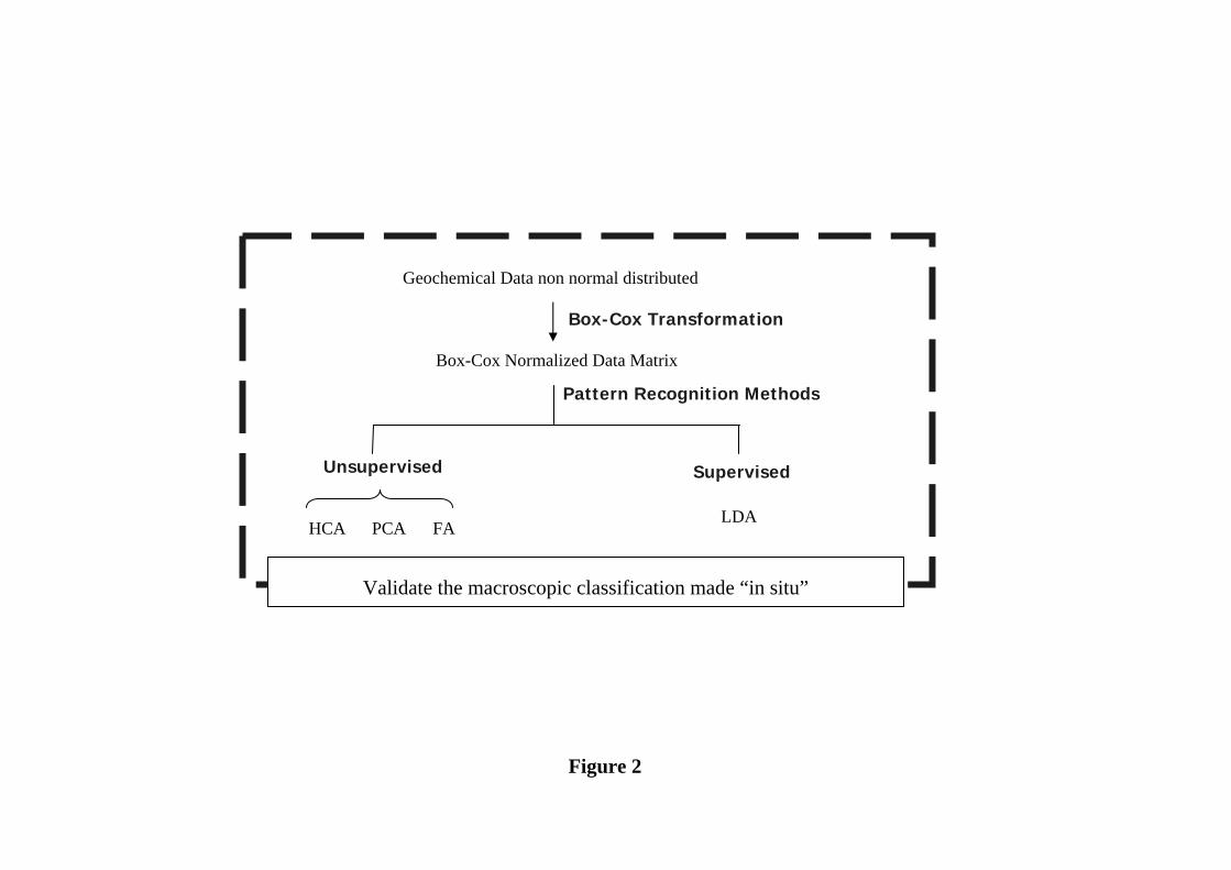
Figure 2 shows the statistical procedure used to the data treatment. Initially, to 2

check the fit of the data to a normal distribution, Kolmogorov-Smirnov, Shapiro-Wilks 3

and skewness score normality tests were applied. In all the cases, statistical evidences at 4

95% confidence interval showed that not all variables are normally distributed. 5

6

FIGURE 2 7

8

In order to transform the data set into normal form, Box-Cox transformation was 9

used [17, 23-25]. To study the correlation structure between normalized variables the 10

Spearman rank-order correlations (Spearman R coefficient) were used, due to the 11

samples are less sensitive to outliers than the Pearson coefficients. 12

13

In all the cases, the univariate and multivariate statistical treatment of the data 14

was performed using: (a) Statgraphic Centurion XV (15.2.05 version) for Windows 15

(Statpoint Technologies Inc, Warrenton, USA) and Matlab Version 7.0.4 R14 (The 16

Mathworks, Inc.) and the PLS Toobox Version 3.0.4 (eigenvector Research, Inc.).. 17

18

19

2.4. Unsupervised pattern recognition methods: Cluster Analysis (HCA), Principal 20

Component (PCA) and Factor Analysis (FA) 21

22

Hierarchical agglomerative HCA was performed on the normalized data set by 23

means of Manhattan (city-block) distance -a particular case of Minkowski distance 24

(taxicab geometry)- as similarity measurement and Ward`s method as amalgamation 25

rule. These criterions have been selected with two objectives: (i) to find at each stage 26

those two clusters whose merger gives the minimum increase in the total within group 27

error sum of squares (Ward objective) and, (ii) to dampen the effect of outliers bearing 28

in mind using city-block distance the average differences across dimensions are not 29

squares. It was applied to the Box-Cox transformed monitoring matrix data set in order 30

to observe the relationship between natural grouping observed and the two criteria of 31

macroscopic classification made (lithologies and alteration patterns). On the other hand 32

in order to verify the natural grouping obtained in HCA, a PCA was applied to the 33

standardized normalized data set. Finally, to reduce the interdependence of the data set 34

9

of standardized normalized variables and to obtain knowledge of the underlying 1

structure of the data, FA was applied. In this case the factorization type used was a 2

principal component which supposes that all of the variability of the data corresponds 3

exclusively to common factors. The orthogonal rotation of the axis defined by PCA, and 4

obtained maximizing (Varimax rotation) produces new groups of variables called 5

varifactors (VFs), which usually group the studied variables in accordance with 6

common features which can include unobservable, hypothetical and/or latent variables 7

[26]. 8

9

2.5. Supervised pattern recognition methods: Linear Discriminant Analysis (LDA) 10

11

This method has been applied in order to obtain a discriminant model that 12

permits us validated the “in situ” macroscopic rock samples classification of the sample 13

assuming the number of groups or classes, as well as, the group membership of each 14

sample taken. Thus, by means of linear discriminant analysis, a discriminant function 15

has been built up for each group on raw data. The classification functions associated to 16

each group defined could be used to determine to which group each sample most likely 17

belongs. In this study, LDA were performed on the Box-Cox transformed measured 18

data. 19

20

3. Results and discussion 21

22

3.1. Macroscopic classification made on the basis of lithology criteria. 23

24

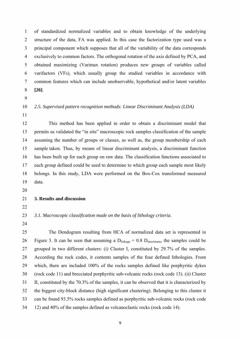
The Dendogram resulting from HCA of normalized data set is represented in 25

Figure 3. It can be seen that assuming a Dlinkage = 0.8 Dmaximum, the samples could be 26

grouped in two different clusters: (i) Cluster I, constituted by 29.7% of the samples. 27

According the rock codes, it contents samples of the four defined lithologies. From 28

which, there are included 100% of the rocks samples defined like porphyritic dykes 29

(rock code 11) and brecciated porphyritic sub-volcanic rocks (rock code 13). (ii) Cluster 30

II, constituted by the 70.3% of the samples, it can be observed that it is characterized by 31

the biggest city-block distance (high significant clustering). Belonging to this cluster it 32

can be found 93.5% rocks samples defined as porphyritic sub-volcanic rocks (rock code 33

12) and 40% of the samples defined as volcanoclastic rocks (rock code 14). 34

10

1

FIGURE 3 2

3

The PCA (made on the basis of eigenvalues > 1 criterion) facilitated the 4

explanation of the original 10 geochemical variables in a reduced space by three sets of 5

the calculated principal components (PCs) which explaining about 73.9% of the total 6

variance. The analysis of the data (see Table 3(a)) shows that PC1 (41.6% of the total 7

variance) is mainly influenced positively by the normalized concentration of Ca, Sr and 8

Ti, and negatively by the normalized concentration of K and Rb. PC2 (19.9% of the 9

total variance) is manly influenced positively by the normalized concentration of Fe, 10

Mn and Zn, and PC3 (which explains the 12.4% of the total variance) influenced 11

positively by Pb, Zn and Cu. 12

13

TABLE 3 14

15

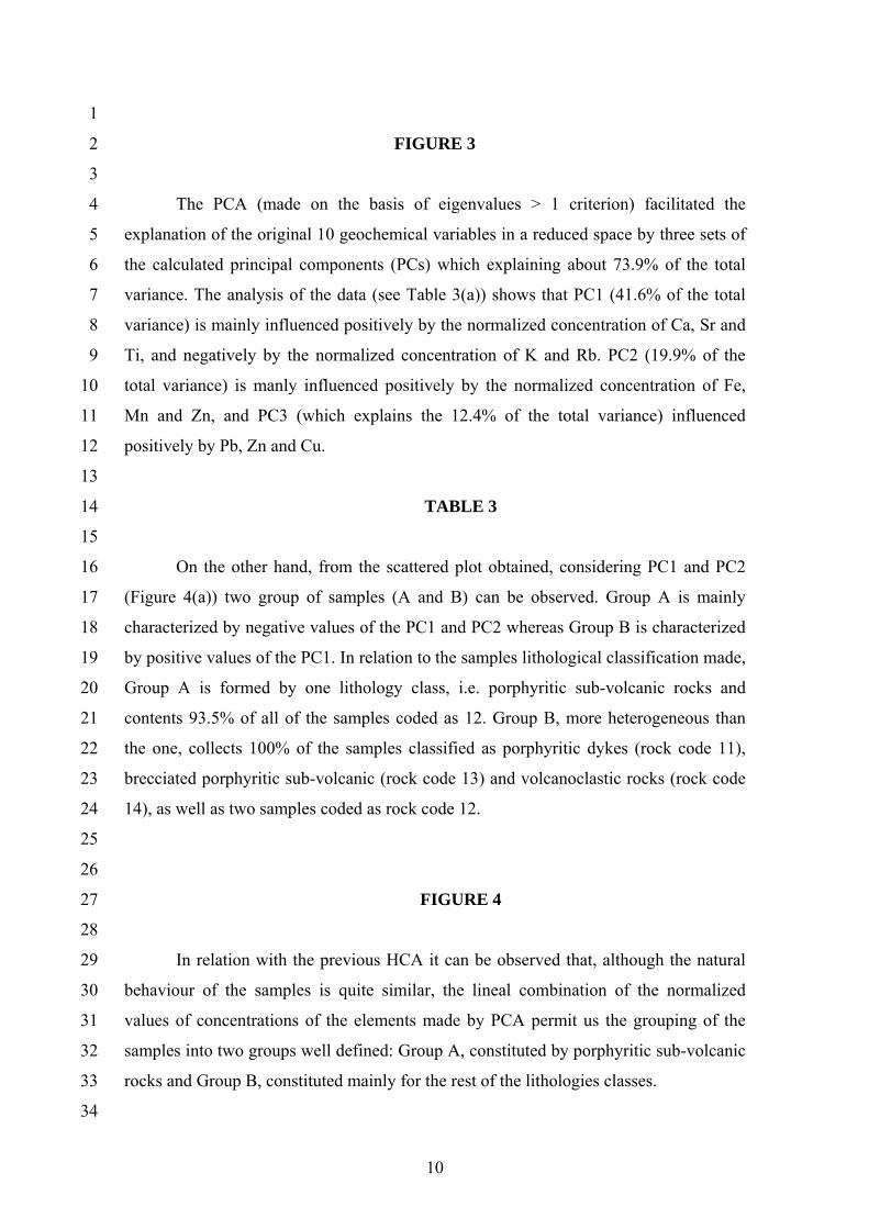
On the other hand, from the scattered plot obtained, considering PC1 and PC2 16

(Figure 4(a)) two group of samples (A and B) can be observed. Group A is mainly 17

characterized by negative values of the PC1 and PC2 whereas Group B is characterized 18

by positive values of the PC1. In relation to the samples lithological classification made, 19

Group A is formed by one lithology class, i.e. porphyritic sub-volcanic rocks and 20

contents 93.5% of all of the samples coded as 12. Group B, more heterogeneous than 21

the one, collects 100% of the samples classified as porphyritic dykes (rock code 11), 22

brecciated porphyritic sub-volcanic (rock code 13) and volcanoclastic rocks (rock code 23

14), as well as two samples coded as rock code 12. 24

25

26

FIGURE 4 27

28

In relation with the previous HCA it can be observed that, although the natural 29

behaviour of the samples is quite similar, the lineal combination of the normalized 30

values of concentrations of the elements made by PCA permit us the grouping of the 31

samples into two groups well defined: Group A, constituted by porphyritic sub-volcanic 32

rocks and Group B, constituted mainly for the rest of the lithologies classes. 33

34

11

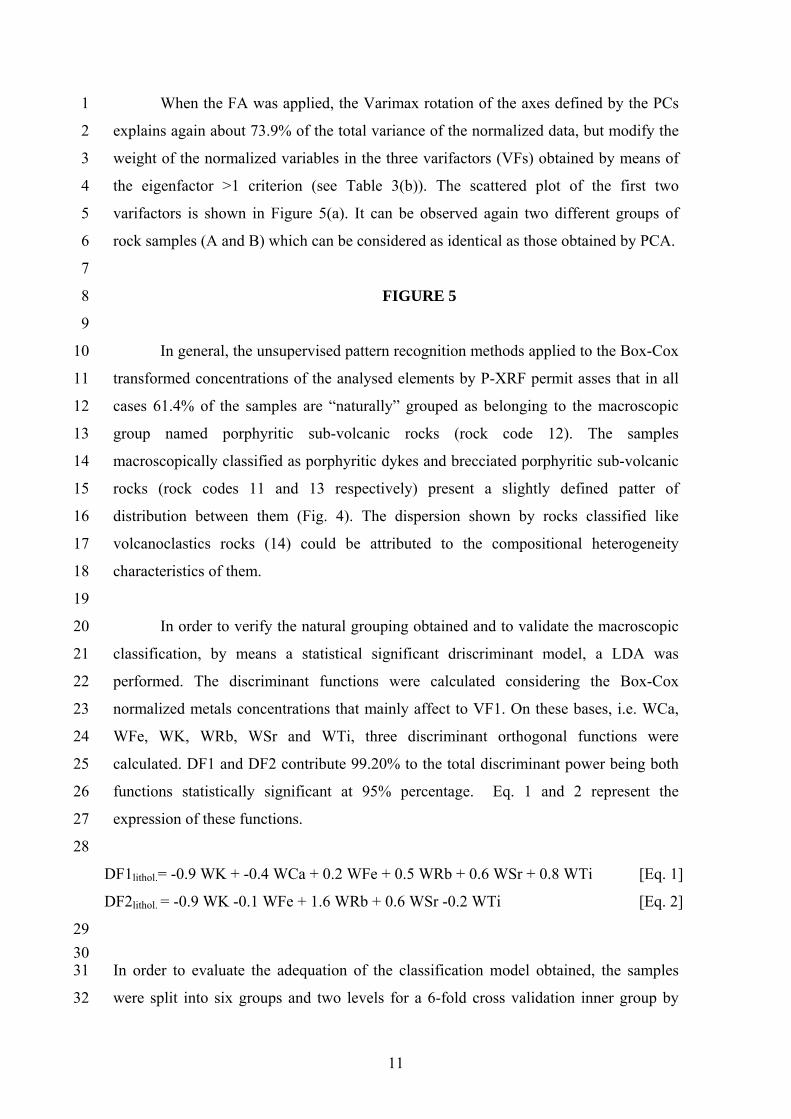
When the FA was applied, the Varimax rotation of the axes defined by the PCs 1

explains again about 73.9% of the total variance of the normalized data, but modify the 2

weight of the normalized variables in the three varifactors (VFs) obtained by means of 3

the eigenfactor >1 criterion (see Table 3(b)). The scattered plot of the first two 4

varifactors is shown in Figure 5(a). It can be observed again two different groups of 5

rock samples (A and B) which can be considered as identical as those obtained by PCA. 6

7

FIGURE 5 8

9

In general, the unsupervised pattern recognition methods applied to the Box-Cox 10

transformed concentrations of the analysed elements by P-XRF permit asses that in all 11

cases 61.4% of the samples are “naturally” grouped as belonging to the macroscopic 12

group named porphyritic sub-volcanic rocks (rock code 12). The samples 13

macroscopically classified as porphyritic dykes and brecciated porphyritic sub-volcanic 14

rocks (rock codes 11 and 13 respectively) present a slightly defined patter of 15

distribution between them (Fig. 4). The dispersion shown by rocks classified like 16

volcanoclastics rocks (14) could be attributed to the compositional heterogeneity 17

characteristics of them. 18

19

In order to verify the natural grouping obtained and to validate the macroscopic 20

classification, by means a statistical significant driscriminant model, a LDA was 21

performed. The discriminant functions were calculated considering the Box-Cox 22

normalized metals concentrations that mainly affect to VF1. On these bases, i.e. WCa, 23

WFe, WK, WRb, WSr and WTi, three discriminant orthogonal functions were 24

calculated. DF1 and DF2 contribute 99.20% to the total discriminant power being both 25

functions statistically significant at 95% percentage. Eq. 1 and 2 represent the 26

expression of these functions. 27

28

DF1lithol.= -0.9 WK + -0.4 WCa + 0.2 WFe + 0.5 WRb + 0.6 WSr + 0.8 WTi [Eq. 1]

DF2lithol. = -0.9 WK -0.1 WFe + 1.6 WRb + 0.6 WSr -0.2 WTi [Eq. 2]

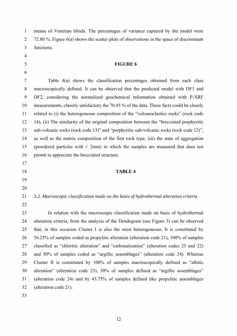
29 30 In order to evaluate the adequation of the classification model obtained, the samples 31

were split into six groups and two levels for a 6-fold cross validation inner group by 32

12

means of Venetian blinds. The percentages of variance captured by the model were 1

72.80 %. Figure 6(a) shows the scatter plots of observations in the space of discriminant 2

functions. 3

4

FIGURE 6 5

6

Table 4(a) shows the classification percentages obtained from each class 7

macroscopically defined. It can be observed that the predicted model with DF1 and 8

DF2, considering the normalized geochemical information obtained with P-XRF 9

measurements, classify satisfactory the 70.45 % of the data. These facts could be closely 10

related to (i) the heterogeneous composition of the “volcanoclastics rocks” (rock code 11

14), (ii) The similarity of the original composition between the “brecciated porphyritic 12

sub-volcanic rocks (rock code 13)” and “porphyritic sub-volcanic rocks (rock code 12)”, 13

as well as the matrix composition of the first rock type, (iii) the state of aggregation 14

(powdered particles with < 2mm) in which the samples are measured that does not 15

permit to appreciate the brecciated structure. 16

17

TABLE 4 18

19

20

3.2. Macroscopic classification made on the basis of hydrothermal alteration criteria 21

22

In relation with the macroscopic classification made on basis of hydrothermal 23

alteration criteria, from the analysis of the Dendogram (see Figure 3) can be observed 24

that, in this occasion Cluster I is also the most heterogeneous. It is constituted by 25

56.25% of samples coded as propylitic alteration (alteration code 21), 100% of samples 26

classified as “chloritic alteration” and “carbonatization” (alteration codes 25 and 22) 27

and 50% of samples coded as “argillic assemblages” (alteration code 24). Whereas 28

Cluster II is constituted by 100% of samples macroscopically defined as “albitic 29

alteration” (alteration code 23), 50% of samples defined as “argillic assemblages” 30

(alteration code 24) and by 43.75% of samples defined like propylitic assemblages 31

(alteration code 21). 32

33

13

The results arisen from PCA (see Figure 4(b)) permit us consider again two 1

groups: Group A constituted by 100% of samples as “albitic alteration” (alteration code 2

23), 45.45% of rock samples assigned as “propylitic alteration (alteration code 21) and 3

50% of rock samples assigned as “argillic assemblages” (alteration code 24). Whereas, 4

Group B includes 68.75% of samples assigned to “propylitic alteration” (alteration code 5

21), as well as samples defined as carbonatization (100%), argillic assemblages (50%) 6

and chloritic (100%) alterations respectively. 7

8

In relation with the information obtain from FA, the scattered plot of the first 9

two varifactors is shown in Figure 5(b). It can be observed again two different groups of 10

rock samples (A and B) which can be defined as those obtained by PCA. Thus, Group A 11

is mainly constituted by 100% of “albitic alteration” (alteration code 23), meanwhile 12

Group B is mainly constituted by samples belonging to “propylitic alteration” 13

(alteration code 21) most of them characterized by high values of VF1 and VF2 and 14

widespread distributed. 15

16

On the other hand, VF1 could be considered in close relation with alteration 17

process, because most of the elements with highest weight, i.e. Ca, K, Rb and Sr could 18

be involved in hydrothermal process [21]. These facts are in good agreement with 19

positive influence of WCa, WSr and WTi, and negative influence of WK and WRb in 20

VF1 found in Group B, constituted by samples with propylitic assemblages and chloritic 21

and carbonatization alterations. Additionally, this is too concordant with the mineralogy 22

(possibly unaltered plagioclase like main mineral phase) of porphyritic (andesitic) 23

dykes. The effect of Ti could be attributed to the presence of ilmenite in the ground 24

mass of dykes. The samples classified as “albitic alteration” has a higher negative 25

influence of WK and WRb, this fact could be due to Na widespread replacement 26

involved in the plagioclase albitization process. This last mineral could be constituted 27

(as initial composition) by significant amounts of K an Rb in its structure. 28

29

VF2 is influenced by the normalized concentrations of base metals as Mn and 30

Zn, while VF3 are influenced by Cu and Pb. These elements could be related with ore 31

mineralization process, nevertheless all the samples show a similar scattered distribution 32

pattern in the diagrams without significance statistical differences inter samples. 33

34

14

Finally, in order to obtain a feasible classification model a PLS-LDA was made. 1

In this case, considering geochemical features i.e. (a) elements closely related to 2

hydrothermal alterations, i.e. WCa, WK, WRb, WSr and (b) the element with 3

economical interest, WCu. On these bases, four discriminant orthogonal functions were 4

calculated. DF1 and DF2 contribute 89.13% to the total discriminant power being both 5

functions the most statistically significant at 95% percentage. Eq. 3 and 4 show the 6

expressions of these functions, 7

8

DF1alt = 0,6 WCa -1,1 WK + WRb + 0.3 WSr – 0.5 WCu [Eq. 3]

DF2alt = WCa + 0.8WK -0.2 WRb -0.6 WSr – 0.1 WCu [Eq. 4]

9

On the other hand, in order to evaluate the adequation of the classification model 10

obtained, the samples were split into six groups and two levels for a 6-fold cross 11

validation inner group by means of Venetian blinds. For this stage the analyses were 12

performed the percentages of variance captured by the model were 72.80 % for 13

lithology and 73.32% for alteration. Figure 5(b) shows the scatter plots of observations 14

in the space of discriminant functions. 15

16

Table 4(b) shows the classification percentages obtained from each type of alteration 17

macroscopically considered. It can be observed that the predicted model considering (i) 18

geological features and (ii) chemical information obtained with P-XRF measurement 19

classify satisfactory the 75 % of the data. The heterogeneity in the predicted types 20

obtained for the samples assigned to “propylitic alteration” could be attributed to the 21

fact that this kind of alteration could content, at micro-scale level, small bodies 22

corresponding to a different alteration process (e.g. carbonatization, chloritic, etc.) not 23

detectable with the equipment used in field campaign sampling. 24

25

26

4. Conclusions 27

28

The statistical treatment of the Box-Cox transformed geological data obtained 29

from “ex-situ” portable X Ray Fluorescence measurements of ore exploratory samples 30

with unsupervised and supervised pattern recognition techniques such as HCA, PCA, 31

FA and LDA has been shown as a helpfully tool for validate the “in-situ” macroscopic 32

15

rock samples classification applied to an exploratory survey in a potential mining area. 1

From the DLA it can be concluded that in relation with the macroscopic rock samples 2

classification based on lithology classes assuming a probability level of 80% the 3

discriminant model obtained confirms correctly 81.8% of the analyzed samples. When 4

the alteration types are considered, the discriminant model obtained permits to confirm 5

four of the five alteration types defined “in situ” (75% of the total samples). Thus, it can 6

be pointed out that the classification assessed could be applied to facilitate and 7

accelerated the remained work necessary to determine the goodness of the ulterior 8

mining exploration. 9

10

On the other hand, the proposed approach could be apply directly “in situ” without pre-11

treatment of the rocks samples during exploratory in those cases in which the 12

characteristic of the samples could be well assessed. 13

14

15

Acknowledgments 16

17

This work was supported by the Spanish project CGL-2006-02594-BTE 18

(founded by Ministry of Science and Innovation = Ministry of Education and Science 19

and Fondo Europeo de Desarrollo Regional, FEDER). The authors are grateful to 20

Minera Las Cenizas S.A. (Cabildo, Chile) for its help during field work and also thanks 21

for the providing access to geological and geochemical information of the studied area. 22

23

24

16

References 1

2

[1] S. Piorek, Trends in Analytical Chemistry 13 (1994), 281-285. 3

[2] A. Argyraki, M. H. Ramsey, P. J. Potts, Analyst (1997), 122, 743-749. 4

[3] P. J. Potts, M. H. Ramsey, J. Carlisle, Journal of Environmental Monitoring 4 5

(2002), 1017-1024. 6

[4] J. Chou, G. Clement, B. Bursavich, D. Elbers, B. Cao, W. Zhou, Environmental 7

Pollution 158 (2010), 2230-2234. 8

[5] P.J. Potts, in J. Potts and M. West (Eds.), Portable X-ray Fluorescence 9

Spectrometry: Capabilities for in-situ analysis, RSC Publishing, London (2008), pp 1-10

12. 11

[6] F. Rosi, A. Burnstock, K. J. Van den Berg, C. Miliani, B. G. Brunetti A. Sgamellotti, 12

Spectrochimica Acta Part A: Molecular and Biomolecular Spectroscopy 71 (2009), 13

1655-1662. 14

[7] G. Van der Snickt, K. Janssens, O. Schalm, C. Aib´eo, H. Kloust, M. Alfelda, X-Ray 15

Spectrom. 39 (2010), 103–111. 16

[8] S. C. Phillips, R. J. Speakman, Journal of Archaeological Science 36 (2009), 1256–17

1263. 18

[9] A. J. Nazaroff, K. M. Prufer, B.L. Drake, Journal of Archaeological Science 37 19

(2010) 885–895. 20

[10] P. L. Drake, N. J. Lawryk, K. Ashley, A. L. Sussell, K. J. Hazelwood, R. Song, 21

Journal of Hazardous Materials 102 (2003) 29–38. 22

[11] C. Kilbride, J. Poole, T.R. Hutchings, Environmental Pollution 143 (2006) 16-23. 23

[12] T. Radu, D. Diamond, Journal of Hazardous Materials 171 (2009) 1168–1171. 24

[13] K. Hürkamp,T. Raab, J. Völkel, Geomorphology 110 (2009) 28–36. 25

[14] M. Ramsey, in J. Potts and M. West (Eds.), Portable X-ray Fluorescence 26

Spectrometry: Capabilities for in-situ analysis, RSC Publishing, London (2008), pp 39-27

55. 28

[15] P. T. Palmer, R. Jacobs, P. E. Baker, K. Ferguson, S. Webber, Journal of 29

Agricultural and Food Chemistry 57 (2009), 2605-2613. 30

[16] F.L. Melquiades, P.S. Parreira, M.J. Yabe, M.Z. Corazza, R. Funfas, C.R. 31

Appoloni, Talanta 73 (2007) 121–126. 32

[17] M. G. Bagur, S. Morales, M. López-Chicano Talanta, 80 (2009), 377-384. 33

17

[18] F. Martín-Peinado, S. Morales-Ruano, M. G. Bagur-González, C. Estepa-Molina, 1

Geoderma 159 (2010), 76-82. 2

[19] M.G. Bagur-González, C. Estepa-Molina, F. Martín-Peinado, S. Morales-Ruano, 3

Journal of Soils and Sediments. DOI: 10.1007/s11368-010-0285-4 (On line from 4

09/2010). 5

[20] V. Maksaev, M. Zentilli, Chilean Strata-bound Cu-(Ag) Deposits: An Overview, in 6

Porter, T.M. (Ed.), Hydrothermal Iron Oxide Copper-Gold & Related Deposits: A 7

Global Perspective, PGC Publishing, Adelaide 2(2002), pp 185-205. 8

[21] H. L. Barnes, Geochemistry of Hydrothermal Ore Deposits, third ed., Wiley, John 9

& Sons, 1997. 10

[22] U.S. EPA, 2006. XRF technologies for measuring trace elements in soil and 11

sediment. Niton XLt 700 Series XRF Analyzer. Innovative technology verification 12

report EPA/540/R-06/004. 13

[23] G.E.P. Box, D.R. Cox, Royal Statistical Association, B26 (1964) 211-250 14

[24] M. Meloun, J. Militký, M. Forina, in PC-Aided Statistical Data Analysis vol. 1 15

(1992) Ellis Horwood, Chichester, United Kingdom. 16

[25] M. Meloun, M. Sâňka, P. Němec, S. Krĭtikova, K. Kupta, Environmental Pollution 17

137 (2005) 273-280 18

[26] C. Pérez-López in Estadística Práctica con STATGRAPHICS, Pearson Education 19

S.A. (2002), Madrid, Spain. 20

21

18

FIGURE CAPTIONS 1

2

Figure 1. Geological map of the Boris Angelo area. 1. Porphyritic dykes 2 & 3. 3

Brecciated porphyritic sub-volcanic rocks 4. Porphyritic sub-volcanic rocks 5. 4

Volcanoclastics rocks 6. Fault 7. Mineralized vein-fault 8. Contact 9. Drill-hole A, B, C 5

and D. Cross section showing the drill holes position and samples location. 6

7

Figure 2. Scheme of the statistical procedure used for data treatment. 8

9

Figure 3. Dendogram resulting from HCA of the Box-Cox normalized data set (R: rock 10

code; A: alteration code; S: sample). 11

12

Figure 4. Scatterplots obtained from PCA of the Box-Cox normalized data set using: 13

(a) rock codes and (b) alteration codes. 14

15

Figure 5. Scatterplots obtained from FA of the Box-Cox normalized data set using (a) 16

rock codes and (b) alteration codes. 17

18

Figure 6. Scatterplots obtained from Discriminant Functions of the Box-Cox 19

normalized data set using (a) rock codes and (b) alteration codes. 20

21

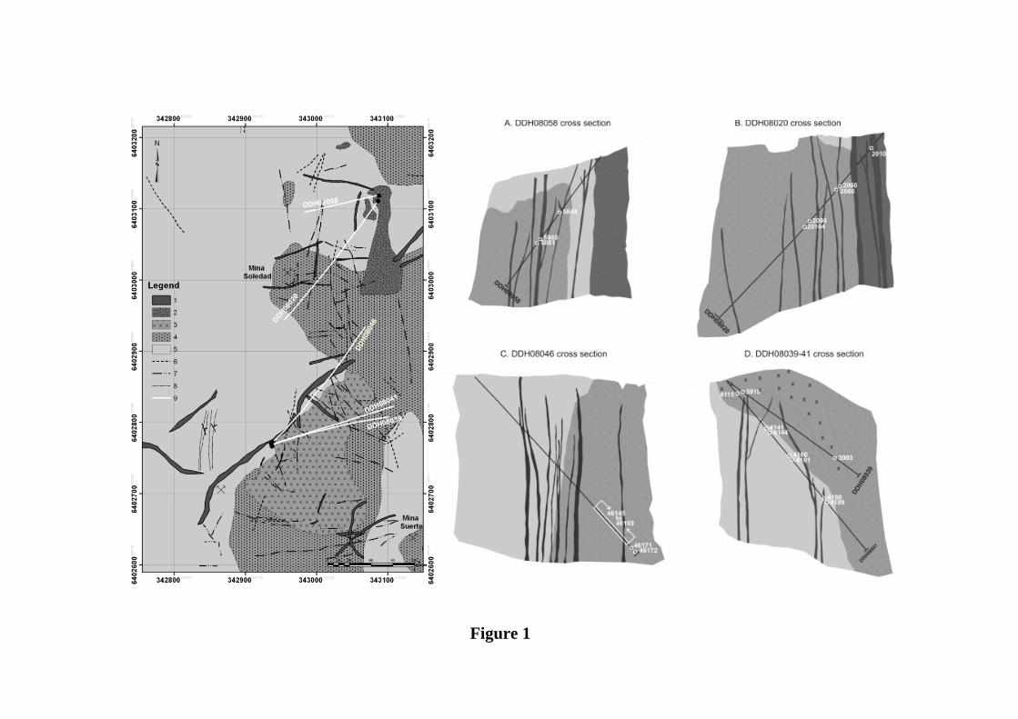
Figure 1

Geochemical Data non normal distributed

Box-Cox Transformation

Box-Cox Normalized Data Matrix

Unsupervised

Pattern Recognition Methods

Supervised

HCA PCA FALDA

Validate the macroscopic classification made “in situ”

Figure 2

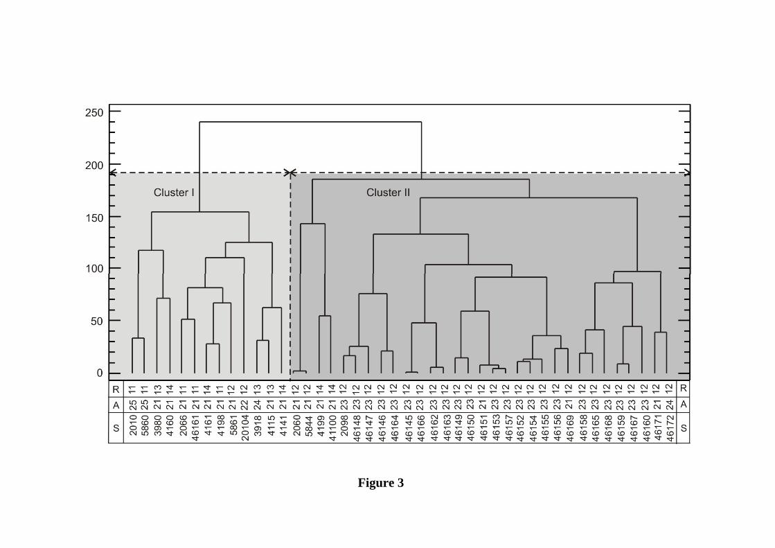
Figure 3

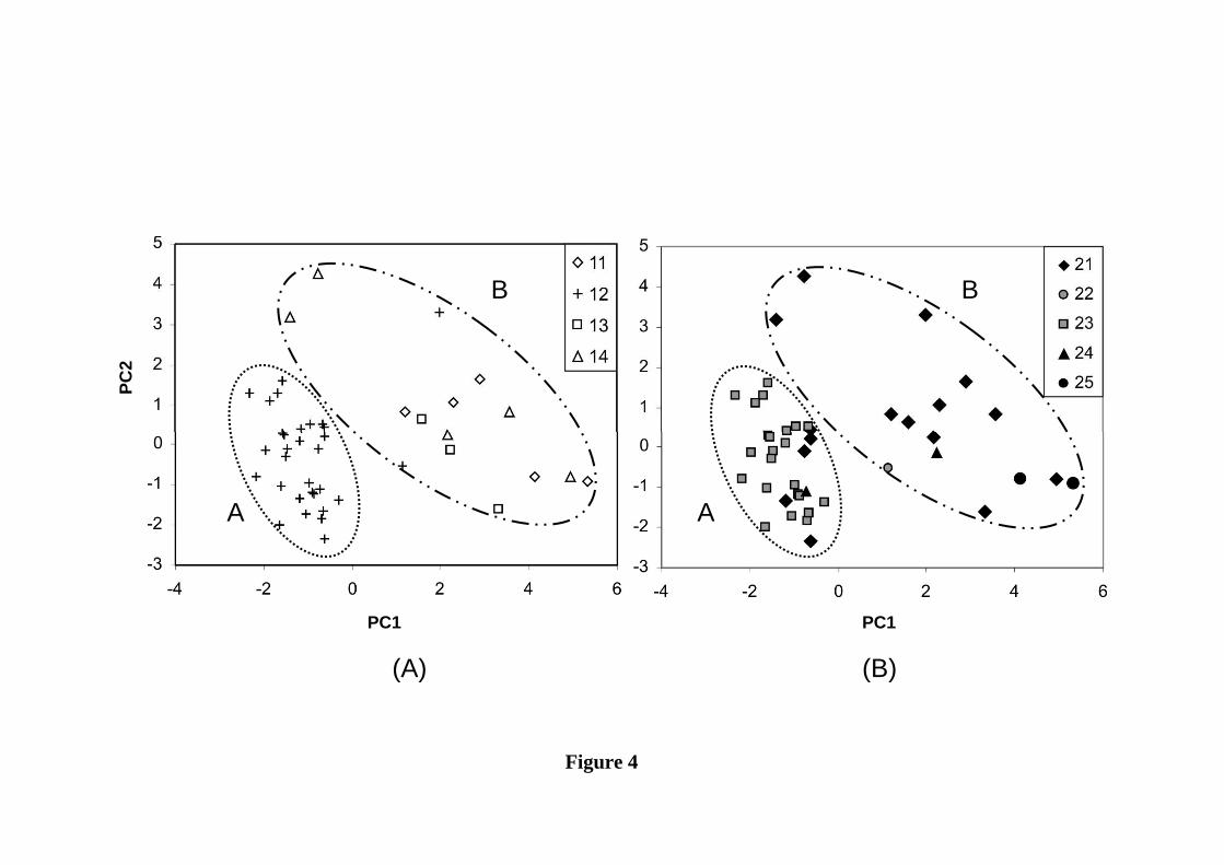
Figure 4

A

B

A

B

(A) (B)

PC1 PC1

PC2

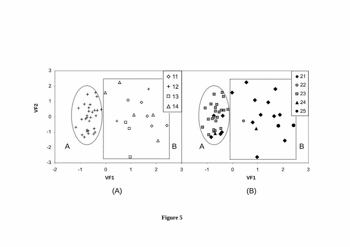
Figure 5

A BA B

(A) (B)

VF1 VF1

VF2

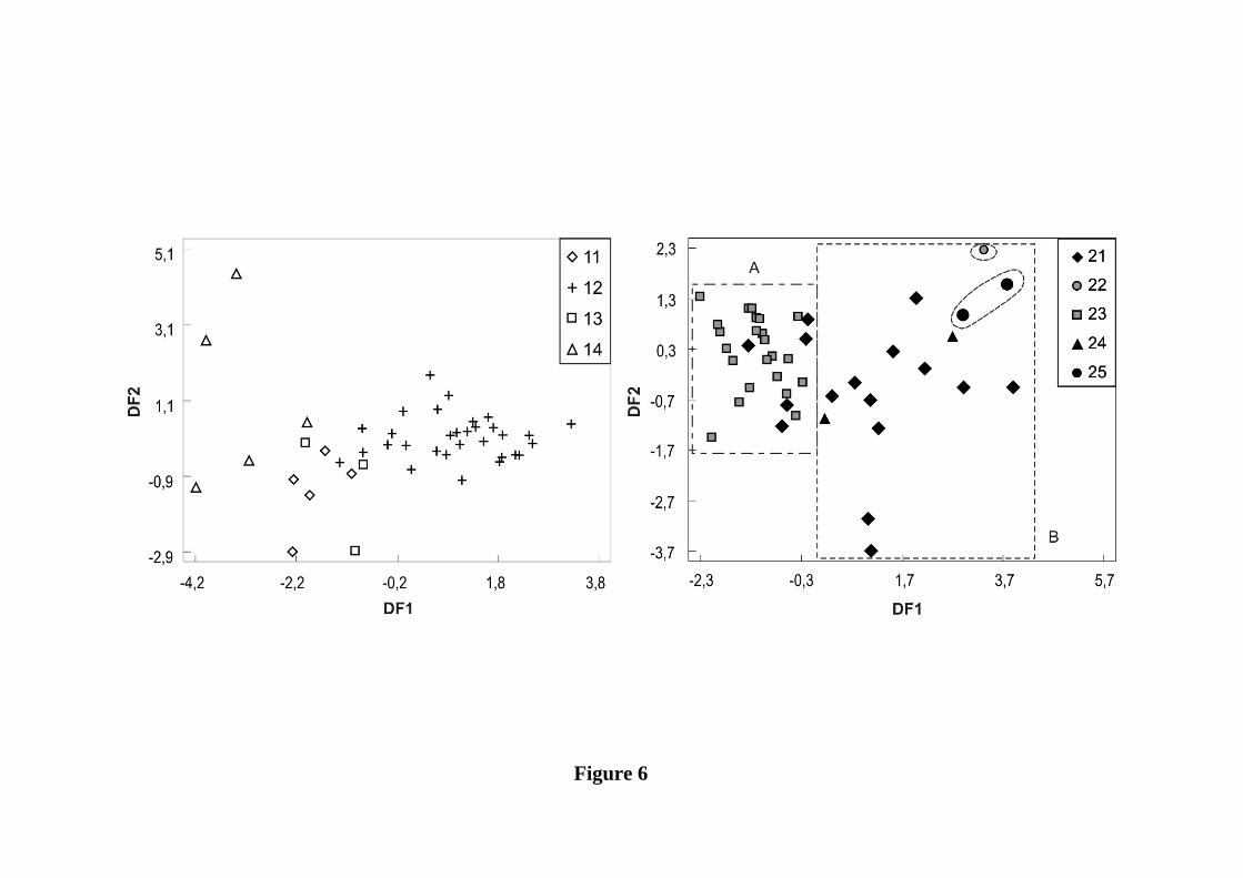
Figure 6

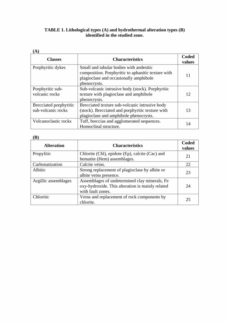
TABLE 1. Lithological types (A) and hydrothermal alteration types (B) identified in the studied zone.

(A)

Classes Characteristics Coded values

Porphyritic dykes Small and tabular bodies with andesitic composition. Porphyritic to aphanitic texture with plagioclase and occasionally amphibole phenocrysts.

11

Porphyritic sub-volcanic rocks

Sub-volcanic intrusive body (stock). Porphyritic texture with plagioclase and amphibole phenocrysts.

12

Brecciated porphyritic sub-volcanic rocks

Brecciated texture sub-volcanic intrusive body (stock). Brecciated and porphyritic texture with plagioclase and amphibole phenocrysts.

13

Volcanoclastic rocks Tuff, breccias and agglomerated sequences. Homoclinal structure. 14

(B)

Alteration Characteristics Coded values

Propylitic Chlorite (Chl), epidote (Ep), calcite (Cac) and hematite (Hem) assemblages. 21

Carbonatization Calcite veins. 22 Albitic Strong replacement of plagioclase by albite or

albite veins presence. 23

Argillic assemblages Assemblages of undetermined clay minerals, Fe oxy-hydroxide. This alteration is mainly related with fault zones.

24

Chloritic Veins and replacement of rock components by chlorite. 25

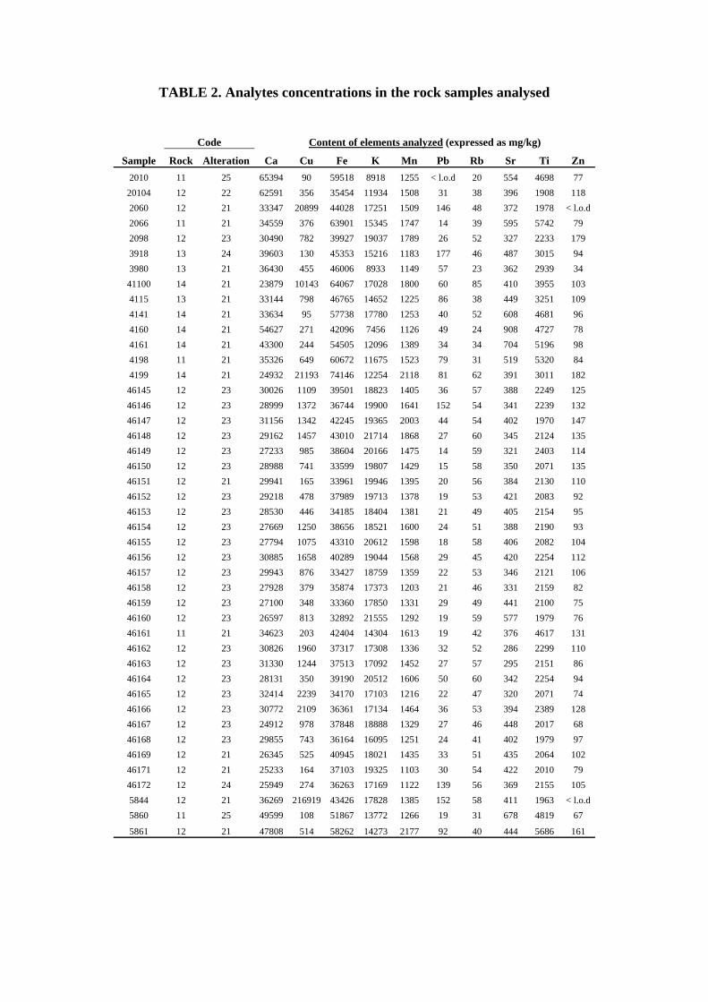
TABLE 2. Analytes concentrations in the rock samples analysed

Code Content of elements analyzed (expressed as mg/kg)

Sample Rock Alteration Ca Cu Fe K Mn Pb Rb Sr Ti Zn 2010 11 25 65394 90 59518 8918 1255 < l.o.d 20 554 4698 77 20104 12 22 62591 356 35454 11934 1508 31 38 396 1908 118 2060 12 21 33347 20899 44028 17251 1509 146 48 372 1978 < l.o.d2066 11 21 34559 376 63901 15345 1747 14 39 595 5742 79 2098 12 23 30490 782 39927 19037 1789 26 52 327 2233 179 3918 13 24 39603 130 45353 15216 1183 177 46 487 3015 94 3980 13 21 36430 455 46006 8933 1149 57 23 362 2939 34 41100 14 21 23879 10143 64067 17028 1800 60 85 410 3955 103 4115 13 21 33144 798 46765 14652 1225 86 38 449 3251 109 4141 14 21 33634 95 57738 17780 1253 40 52 608 4681 96 4160 14 21 54627 271 42096 7456 1126 49 24 908 4727 78 4161 14 21 43300 244 54505 12096 1389 34 34 704 5196 98 4198 11 21 35326 649 60672 11675 1523 79 31 519 5320 84 4199 14 21 24932 21193 74146 12254 2118 81 62 391 3011 182 46145 12 23 30026 1109 39501 18823 1405 36 57 388 2249 125 46146 12 23 28999 1372 36744 19900 1641 152 54 341 2239 132 46147 12 23 31156 1342 42245 19365 2003 44 54 402 1970 147 46148 12 23 29162 1457 43010 21714 1868 27 60 345 2124 135 46149 12 23 27233 985 38604 20166 1475 14 59 321 2403 114 46150 12 23 28988 741 33599 19807 1429 15 58 350 2071 135 46151 12 21 29941 165 33961 19946 1395 20 56 384 2130 110 46152 12 23 29218 478 37989 19713 1378 19 53 421 2083 92 46153 12 23 28530 446 34185 18404 1381 21 49 405 2154 95 46154 12 23 27669 1250 38656 18521 1600 24 51 388 2190 93 46155 12 23 27794 1075 43310 20612 1598 18 58 406 2082 104 46156 12 23 30885 1658 40289 19044 1568 29 45 420 2254 112 46157 12 23 29943 876 33427 18759 1359 22 53 346 2121 106 46158 12 23 27928 379 35874 17373 1203 21 46 331 2159 82 46159 12 23 27100 348 33360 17850 1331 29 49 441 2100 75 46160 12 23 26597 813 32892 21555 1292 19 59 577 1979 76 46161 11 21 34623 203 42404 14304 1613 19 42 376 4617 131 46162 12 23 30826 1960 37317 17308 1336 32 52 286 2299 110 46163 12 23 31330 1244 37513 17092 1452 27 57 295 2151 86 46164 12 23 28131 350 39190 20512 1606 50 60 342 2254 94 46165 12 23 32414 2239 34170 17103 1216 22 47 320 2071 74 46166 12 23 30772 2109 36361 17134 1464 36 53 394 2389 128 46167 12 23 24912 978 37848 18888 1329 27 46 448 2017 68 46168 12 23 29855 743 36164 16095 1251 24 41 402 1979 97 46169 12 21 26345 525 40945 18021 1435 33 51 435 2064 102 46171 12 21 25233 164 37103 19325 1103 30 54 422 2010 79 46172 12 24 25949 274 36263 17169 1122 139 56 369 2155 105 5844 12 21 36269 216919 43426 17828 1385 152 58 411 1963 < l.o.d5860 11 25 49599 108 51867 13772 1266 19 31 678 4819 67

5861 12 21 47808 514 58262 14273 2177 92 40 444 5686 161

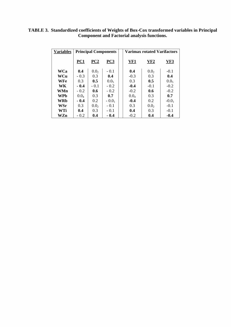
TABLE 3. Standardized coefficients of Weights of Box-Cox transformed variables in Principal Component and Factorial analysis functions.

Variables Principal Components Varimax rotated Varifactors PC1 PC2 PC3 VF1 VF2 VF3

WCa 0.4 0.02 - 0.1 0.4 0.02 -0.1 WCu - 0.3 0.3 0.4 -0.3 0.3 0.4 WFe 0.3 0.5 0.05 0.3 0.5 0.05 WK - 0.4 - 0.1 - 0.2 -0.4 -0.1 -0.2

WMn - 0.2 0.6 - 0.2 -0.2 0.6 -0.2 WPb 0.04 0.3 0.7 0.04 0.3 0.7 WRb - 0.4 0.2 - 0.01 -0.4 0.2 -0.01 WSr 0.3 0.02 - 0.1 0.3 0.02 -0.1 WTi 0.4 0.3 - 0.1 0.4 0.3 -0.1 WZn - 0.2 0.4 - 0.4 -0.2 0.4 -0.4

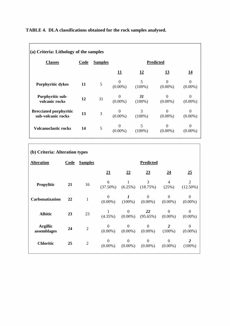
TABLE 4. DLA classifications obtained for the rock samples analysed.

(a) Criteria: Lithology of the samples

Classes Code Samples Predicted

11

12

13

14

Porphyritic dykes 11 5 0 (0.00%)

5 (100%)

0 (0.00%)

0 (0.00%)

Porphyritic sub-volcanic rocks 12 31 0

(0.00%) 31

(100%) 0

(0.00%) 0

(0.00%) Brecciated porphyritic

sub-volcanic rocks 13 3 0 (0.00%)

3 (100%)

0 (0.00%)

0 (0.00%)

Volcanoclastic rocks 14 5 0 (0.00%)

5 (100%)

0 (0.00%)

0 (0.00%)

(b) Criteria: Alteration types Alteration Code Samples Predicted

21 22 23 24

25

Propylitic 21 16 6 (37.50%)

1 (6.25%)

3 (18.75%)

4 (25%)

2 (12.50%)

Carbonatization 22 1 0 (0.00%)

1 (100%)

0 (0.00%)

0 (0.00%)

0 (0.00%)

Albitic 23 23 1 (4.35%)

0 (0.00%)

22 (95.65%)

0 (0.00%)

0 (0.00%)

Argillic

assemblages 24 2 0 (0.00%)

0 (0.00%)

0 (0.00%)

2 (100%)

0 (0.00%)

Chloritic 25 2 0 (0.00%)

0 (0.00%)

0 (0.00%)

0 (0.00%)

2 (100%)