1

Topic 5 - Joint distributions and the CLT• Joint distributions

– Calculation of probabilities, mean and variance– Expectations of functions based on joint distributions

• Central Limit Theorem – Sampling distributions

• Of the mean• Of totals

22

• Often times, we are interested in more than one random variable at a time.

• For example, what is the probability that a car will have at least one engine problem and at least one blowout during the same week?

• X = # of engine problems in a week

• Y = # of blowouts in a week

• P(X ≥ 1, Y ≥ 1) is what we are looking for

• To understand these sorts of probabilities, we need to develop joint distributions.

33

Discrete distributions

• A discrete joint probability mass function is given by

f(x,y) = P(X = x, Y = y)where

all ( , )

all ( , )

all ( , )

1. ( , ) 0 for all ,

2. ( , ) 1

3. (( , ) ) ( , )

4. ( ( , )) ( , ) ( , )

x y

x y A

x y

f x y x y

f x y

P X Y A f x y

E h X Y h x y f x y

44

Return to the car example

• Consider the following joint pmf for X and Y

• P(X ≥ 1, Y ≥ 1) =

• P(X ≥ 1) = • E(X + Y) =

X\Y 0 1 2 3 4

0 1/2 1/16 1/32 1/32 1/32

1 1/16 1/32 1/32 1/32 1/32

2 1/32 1/32 1/32 1/32 1/32

55

Joint to marginals• The probability mass functions for X and Y individually

(called marginals) are given by

• Returning to the car example:

fX(x) =

fY(y) =

E(X) =

E(Y) =

all all ( ) ( , ), ( ) ( , )X Yy x

f x f x y f y f x y

66

Continuous distributions

• A joint probability density function for two continuous random variables, (X,Y), has the following four properties:

- -

- -

1. ( , ) 0 for all ,

2. ( , ) 1

3. (( , ) ) ( , )

4. ( ( , )) ( , ) ( , )

A

f x y x y

f x y dxdy

P X Y A f x y dxdy

E h X Y h x y f x y dxdy

77

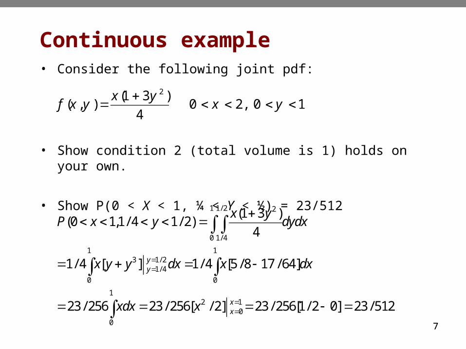
Continuous example• Consider the following joint pdf:

• Show condition 2 (total volume is 1) holds on your own.

• Show P(0 < X < 1, ¼ < Y < ½) = 23/512

2(1 3 )( , ) 0 2, 0 1

4x y

f x y x y

1 1/ 2 2

0 1/ 4

1 13 1/ 2

1/ 4

0 0

12 1

0

0

(1 3 )(0 1,1/ 4 1/ 2)

4

1/ 4 [ ] 1/ 4 [5 / 8 17 / 64]

23/ 256 23/ 256[ / 2] 23/ 256[1/ 2 0] 23/ 512

yy

xx

x yP x y dydx

x y y dx x dx

xdx x

88

Joint to marginals

• The marginal pdfs for X and Y can be found by

• For the previous example, find fX(x) and fY(y).

( ) ( , ) , ( ) ( , )X Yf x f x y dy f y f x y dx

1 23 1

0

0

(1 3 )( ) = / 4[ ] = / 4[2 0] / 2

4y

x y

x yf x dy x y y x x

2 22 2 2

2 20

0 0

2

(1 3 ) (1 3 ) (1 3 )( ) = = [ / 2]

4 4 4

1 3

2

xy x

x y y yf y dx xdx x

y

99

Independence of X and Y

• The random variables X and Y are independent if

– f(x,y) = fX(x) fY(y) for all pairs (x,y).

• For the discrete clunker car example, are X and Y independent?

• For the continuous example, are X and Y independent?

2 2 2(1 3 ) (1 3 ) (1 3 )( , ) ( ) ( ) ( )

4 2 2 4x y

x y x y x yf x y f x f y

1010

Sampling distributions• We assume that each data value we collect represents a

random selection from a common population distribution.

• The collection of these independent random variables is called a random sample from the distribution.

• A statistic is a function of these random variables that is used to estimate some characteristic of the population distribution.

• The distribution of a statistic is called a sampling distribution.

• The sampling distribution is a key component to making inferences about the population.

Statistics used to infer parametersWe take samples and calculate statistics to make inferences about the population parameters.

Sample Population

Mean

Std. Dev.

Variance

Proportion

11

x

s 2s 2

p̂ p

1212

StatCrunch example• StatCrunch subscriptions are sold for 6 months ($5) or 12

months ($8).

• From past data, I can tell you that roughly 80% of subscriptions are $5 and 20% are $8.

• Let X represent the amount in $ of a purchase.

• E(X) =

• Var(X) =

1313

StatCrunch example continued• Now consider the amounts of a random sample of two

purchases, X1, X2.

• A natural statistic of interest is X1 + X2, the total amount of the purchases.

Outcomes

X1 + X2 Probability

5,5

5,8

8,5

8,8

X1 + X2

Probability

1414

StatCrunch example continued

• E(X1 + X2) =

• E([X1 + X2]2) =

• Var(X1 + X2) =

1515

StatCrunch example continued

• If I have n purchases in a day, what is– my expected earnings?– the variance of my earnings?– the shape of my earnings distribution for large n?

• Let’s experiment by simulating 10,000 days with 100 purchases per day using StatCrunch.

1616

Simulation instructions

• Data > Simulate data > Binomial

• Specify Rows to be 10000, Columns to be 1, n to be 100 and p to be .2. This will give you a new column called Binomial1

• To compute the total for each day, go to Data > Transform data and enter the expression, 8*Binomial1+5*(100-Binomial1). This will add a new column to the data table.

• Make a histogram and set the bin width to 1 for best results.

• For the new sum column, do a histogram and a QQ plot. Both should verify normality!

StatCrunch

17

Should result in a dataset like this

1818

Central Limit Theorem• We have just illustrated one of the most important

theorems in statistics.

• As the sample size, n, becomes large the distribution of the sum of a random sample from a distribution with mean and variance 2 converges to a Normal distribution with mean n and variance n2.

• A sample size of at least 30 is typically required to use the CLT (arguable in the general statistics community).

• The amazing part of this theorem is that it is true regardless of the form of the underlying distribution.

1919

Airplane example

• Suppose the weight of an airline passenger has a mean of 150 lbs. and a standard deviation of 25 lbs.

• What is the probability the combined weight of 100 passengers will exceed the maximum allowable weight of 15,500 lbs?

• How many passengers should be allowed on the plane if we want this probability to be at most 0.01?

What are the probabilities at n = 99?The mean is The variance isThe standard deviation is

20

99*150 14850299*25 61850

61875 248.75

( 15500)

0.004487TOTP X

2121

The distribution of the sample means

• For constant c, E(cY) = cE(Y) and Var(cY) = c2Var(Y)

•

•

• The CLT says that for large samples, is approximately normal with a mean of and a variance of 2/n.

• So, the variance of the sample mean decreases with n.

X

22

2 2

1 1 1( ) ( ) ( )Var X Var x Var x n

n n n n

What are the probabilities we get asample average at some level?If the parent population is assumed with a mean of 150 lbs. and a standard deviation of 25 lbs., what’s the probability we get a sample average below 141 with a sample size of 30?

Talking about thesampling distribution,the mean is 150 and thestandard deviation is

22

254.5644

30

Sampling distribution applet

• In StatCrunch, go to the “Applets” tab and click on “sampling distributions”. It will demonstrate how any parent distribution will converge to normal with larger, repeated samples.

• The closer the parent is to symmetrical, the quicker the sampling distribution will converge.

The additional file for Topic 5 has discussion and examples on both sampling distributions and joint probability distributions. There are also additional examples of double integration.

2323