Embed Size (px)
Citation preview
1
TRANSPORT OF WATER BY ADVECTION AND DIFFUSION 1
By A. T. Corey and P. D. Corey 2
May 26, 2016 3
ABSTRACT 4
This investigation is concerned with transport of discrete particles in water 5
solutions occupying porous media. The solid boundary of a water solution is 6
employed as a frame of reference for defining particle velocities so that velocity 7
of the boundary is defined as zero in this frame of reference. Experimental 8
evidence shows that net flux of fluid particles is the sum of advection and 9
diffusion. Flux refers to velocity of a reference volume of a water solution as a 10
whole, not velocity of individual particles. The term “osmosis” is often used to 11
describe a combination of advection and diffusion. Advection in a particular 12
direction is flux of fluid particles driven by a force proportional to normal surface 13
forces in that direction on the boundary of a reference volume of a liquid water 14
solution as a whole, as well as body forces in that direction acting on mass within 15
a reference volume. Diffusion of liquid water particles in a particular direction is 16
flux proportional to the directional derivative of kinetic energy of water particles 17
per unit volume. Kinetic energy is due to particle velocities relative to the 18
boundary velocity. Models describing mass transport of fluid particles in water 19
solutions based on a definition of diffusion as flux of fluid particles relative to 20
mean flux do not predict fluxes relative to the solution boundary. Functions 21
describing conditions for fluid equilibrium do not describe fluid flux. 22
23
OBJECTIVES 24
25
An objective of this investigation is to show that net flux of a liquid water 26
solution is the sum of advection and diffusion. Another objective is to show that 27
definition of diffusion as a flux relative to mean flux is flawed, and the concept of 28
non-equilibrium thermodynamics for describing fluid flux is also flawed. 29

2
A particle is a mass that translates as a unit in a solution. No assumption 1
is made regarding its structure. For example, a particle could be a gas molecule 2
in a gaseous solution or a water cluster in a water solution. 3
Fluids, as defined here, are not treated as continua, as often is the case 4
for fluids discussed in fluid dynamics texts. Transport of particles in a soil water 5
solution is frequently assumed proportional to a directional derivative of a single 6
potential even though net flux in a particular direction may be driven by 7
directional derivatives of at least two significant potentials, that is, potentials 8
referring to energy associated with advection and energy associated with 9
diffusion. 10
A potential is the energy of particles per unit volume (or per unit mass) of 11
a solution. When referring to advection the potential refers to energy per unit 12
volume of particles in a reference volume of the solution as a whole, and when 13
referring to diffusion, a potential is energy per unit mass of a set of particles in a 14
reference volume. Net flux is equal to velocity of the centroid of a reference 15
volume as a whole and is equal to the sum of advection and diffusion. 16
The term kinetic energy refers to energy associated with particle velocities 17
in a frame of reference relative to the solid boundary of the fluid solution. A 18
directional derivative of a potential evaluates the driving force in a particular 19
direction. Kinetic energy, as defined here, is employed as a potential for diffusion 20
with dimensions of energy per unit mass. 21
Although most current investigators of flow in porous media employ the 22
term gradient when referring to a directional derivative, the distinctions in 23
meaning (for example) between dx
dp and p are emphasized here. A directional 24
derivative is used to evaluate a force driving particles in any particular direction at 25
a point in a fluid system; whereas a gradient evaluates the maximum driving 26
force at a particular point. Flux components described in most current literature 27
dealing with flux of liquid solutions in porous media are rarely the largest flux 28
components possible at points in a porous medium, although the driving force is 29
often incorrectly evaluated as a gradient of a potential. 30
3
To illustrate principles applying to net flux of liquid water in porous media, 1
a de-ionized liquid water solution occupying a stable porous medium is examined 2
theoretically and experimentally. Such a water solution is rarely, if ever, found in 3
soils or aquifers because water solutions found in soils or aquifers are not 4
de-ionized. A de-ionized water solution is examined here; because theoretically 5
only advection and diffusion of water particles are involved in this special case. It 6
is easier to focus attention on principles that apply to advection and diffusion of 7
liquid water for this special case. 8
Summing fluxes due to advection and diffusion is not sufficient to 9
evaluate net flux of water solutions in general. Cases where mixed fluid 10
phases (where each phase is often treated as a separate continuum) are not 11
discussed here. Flux of compressible fluids, e.g., air or other gases, in 12
particular, is not discussed. The reader is referred to the text by Corey, A.T. 13
1994 for a discussion of advection of multiple phases. Driving force due to 14
directional derivatives of electrical potential is also not discussed. The reader 15
is referred to papers by Kemper, W.D. 1960, Olsen, H.W. 1985, and Malusis, 16
M.A., C.H. Shackelford and H.W. Olsen 2001 for a discussion of electrical 17
potentials in soil solutions. 18
This investigation ignores the effect of de-ionized water on the 19
geometry of fluid channels in porous media, such as, clay swelling in soils. 20
Experiments with advection and diffusion in de-ionized liquid water solutions 21
occupying porous media (unaffected by a liquid water solution) are cited. 22
Conclusions based on theoretical analyses are presented if they have been 23
verified by published experimental observations. 24
25
BACKGROUND 26
27
The earliest literature dealing with flux of liquid water through porous 28
media is by Henri Darcy 1856. A packed sand bed employed by Darcy in his 29
4
experiments contained fluid channels small enough that inertial resistance is 1
negligible, but large enough that net flux is dominated by advection. Inertial 2
resistance is neglected because net flux of water through the packed sand bed is 3
sufficiently small that inertia is not a significant factor. Du Plessis, J.P. 1994, has 4
provided rigorous theoretical and experimental research describing conditions 5
where this assumption is justified. 6
Darcy described net flux employing macroscopic variables, and described 7
the driving force for advection of a liquid water solution as the directional 8
derivative of hydraulic head. The term macroscopic implies that the flux 9
measured is averaged over a cross-section that includes solids as well as a liquid 10
solution. Hydraulic head is a potential, the directional derivative of which is 11
dimensionless, representing force per weight of water solution. 12
An equation, analogous to Darcy’s equation, written in macroscopic units 13
with driving force per volume, rather than per weight of water solution is given by: 14
15
)( gpdx
dK
x
aq . (1) 16
17
The flux vector evaluated by Eq. (1) is volume flux (referring to the solution as a 18
whole) per unit area per unit time, that is, it has dimensions of velocity. 19
Eq. (1) is often called Darcy’s equation where the body force, g, is gravity. 20
Orientation of the cross-section, through which flux is evaluated, is arbitrary and 21
the variables employed are macroscopic. K is a coefficient called hydraulic 22
conductivity relating advective flux (in a direction normal to the cross-section 23
selected) to its driving force; g is a scalar representing potential energy per mass 24
resulting from position in a gravitational field, p is pressure, and ρ is fluid 25
density. 26
Directions of flux components evaluated by Eq. (1) are determined by 27
directional derivatives of the sum in parentheses, called piezometric pressure. 28
5
Fluxes evaluated by Eq. (1) represent components of flux driven by force 1
evaluated with directional derivatives, not gradient operators. 2
An equation with a form similar to Eq. (1) may refer to a force unrelated to 3
gravity, e.g., a force driving diffusion. Fluxes evaluated by equations with the 4
same form are additive because each flux can be expressed with the same 5
dimensions by choosing a coefficient with appropriate dimensions. However, 6
potentials associated with advection and diffusion cannot be added because they 7
are different functions of porous media. 8
Driving forces for advection should be described as force per unit volume, 9
because the potentials involved include energy resulting from surface forces that 10
cannot be evaluated over an element of mass. Diffusion should be described as 11
force per unit mass, because the component of flux evaluated is flux of particular 12
particles, and the volume occupied by a set of particles is unknown. 13
The sum in parentheses in Eq. (1) is frequently referred to as piezometric 14
pressure p*, a variable with dimensions of energy per volume Experience shows 15
that Eq. (1) provides an acceptable evaluation of net flux in a particular direction 16
in most agricultural soils and aquifers, because diffusion is usually an 17
insignificant mechanism of transport compared to advection in soils and aquifers. 18
The coefficient employed in Eq. (1) is a function of fluid viscosity, as well 19
as media properties, and should be adjusted for viscosity, a function of 20
temperature. For advective flux in horizontal directions, the gradient of 21
piezometric pressure reduces to a gradient of pressure only. 22
In evaluating a flux component with Eq. (1) in a real system, one may 23
attempt to evaluate a flux component in a direction parallel to bedding planes of a 24
geologic earth formation or perhaps through a membrane in a normal direction. 25
Fluxes evaluated are in a direction chosen for convenience. When flux 26
components resulting from directional derivatives, in general, are combined, they 27
should refer to the same direction. Vectors such as fluxes or forces are indicated 28
by symbols with bold font in this investigation. 29
6
Although, experience shows that Eq. (1) provides an acceptable 1
evaluation of net flux in a particular direction over a large range of conditions, 2
Eq. (1) fails to describe net flux in media such as membranes in living cells, shale 3
layers where the petroleum industry currently extracts natural gas, or compacted 4
clay layers used to retain dangerous chemicals in mining waste storage dumps. 5
Eq. (1) also does not describe advective flux of compressible fluids through 6
porous media, e. g., gases, because it is impossible for a pressure difference to 7
exist in gases without inducing diffusion as well as advection, and causing 8
slippage at solid boundaries. 9
10
Advection in porous media 11
The definition of advection given above is a flux due to surface force on a 12
reference volume of a liquid solution as a whole, plus a body force on mass 13
within a reference volume. This defines advection at a point in a fluid system 14
because a reference volume is defined at a point in space, that is, the centroid of 15
a reference volume. Experience shows that if a finite advection is found at a point 16
in the channels within a porous medium, advection will be found at all points 17
within channels occupied by a liquid solution. However, fluxes of liquid solutions 18
as a whole apparently approach zero at solid boundaries. This does not imply 19
that velocity of individual particles is necessarily zero at a boundary. 20
Flux velocities at other points in a liquid water solution are found to be 21
inversely proportional to the distance normal to the surface of solids. Such 22
velocity distributions, called viscous flux, result in angular deformation of 23
reference volumes, and resistance to viscous flux is found to be proportional to 24
rate of angular deformation of reference volumes. 25
26
Diffusion through plant membranes 27
Plant scientists often regard net flux of particles through plant membranes 28
as being proportional to directional derivatives of activity, where activity is a 29
potential with dimensions of energy per unit mass, referring to a particular 30
7
particle. Although transport of individual particles evaluated by the directional 1
derivatives of potentials with dimensions of energy per unit mass evaluates mass 2
transport due to diffusion, mass transport due to advection is not evaluated. 3
Many plant scientists apparently consider that directional derivatives of 4
activity evaluate forces that can drive advection, as well as diffusion. They 5
apparently believe surface forces, e.g., pressure and viscous resistance, are 6
accounted for by employing directional derivatives of activity to evaluate forces 7
driving advection as well as diffusion. 8
However, pressure is normal force per unit area and viscous resistance is 9
tangential surface force per unit area. Surface force can be evaluated on the 10
surface of volumes, not on elements of mass. Consequently, there is no logical 11
way to apply activity as a potential for evaluating advection. Such a potential is 12
useful for evaluating mass flux of particular particles, a process defined as 13
diffusion. 14
When plant scientists discover an occasional particle with insufficient 15
activity to have arrived inside a plant by diffusion, they often assume the energy 16
difference allowing it to have passed a plant membrane must have been created 17
by the pumping action of living cells. Apparently, many plant scientists think plant 18
membranes do not permit advection that could provide transport of particles 19
larger than water clusters through root hairs without pumping by a vital process. 20
Advective fluxes capable of allowing particles larger than water particles to 21
pass through plant membranes against an activity difference, unrelated to a 22
process of living organisms, are possible. However, because fluid channels 23
through root hairs are likely to be small enough to impede advection, diffusion is 24
probably the primary mechanism of transport through root hairs in most cases. 25
26
Diffusion 27
The scientific community has long recognized that diffusion as well as 28
advection contributes significantly to net flux in porous media having very small 29
fluid channels. Investigators have differed concerning the definition of diffusion. It 30
8
was originally regarded as a flux of particles relative to a solid matrix, and later 1
incorrectly defined as flux relative to a moving stream. 2
The earliest experiments dealing specifically with diffusion are 3
experiments conducted by Graham, T. 1833 regarding diffusion of gases through 4
plaster-of-Paris, a porous medium with extremely small fluid channels. Graham 5
likely regarded advection through plaster-of-Paris to be negligible compared to 6
diffusion. 7
To insure diffusion was the flux measured in his experiments, Graham 8
manually held the pressure of each gas employed equal on both sides of a 9
porous plug of plaster of Paris and measured flux components through a cross-10
section normal to gravity. Theoretically, such flux components are due to 11
diffusion only. 12
Graham evidently regarded diffusion as flux of particular particles relative 13
to the solid material forming the boundary of gaseous mixtures. The fluxes he 14
measured are with respect to the porous medium used for his experiments, not 15
flux relative to a moving stream. Graham regarded diffusion as flux of particular 16
particles because he stated that diffusive flux is inversely proportional to the 17
square root of particle mass. 18
Experience of numerous subsequent investigators has confirmed 19
Graham’s findings, e.g., Hoogschagen, J. 1953, and Knaff, G. and 20
E.U. Schlunder 1985. But many investigators have also discovered that diffusive 21
flux of liquid water particles is found experimentally to increase with temperature, 22
e. g., the diffusive fluxes measured by Corey, A.T., W.D. Kemper and J.H. Dane. 23
2010. 24
25
Fick’s equation 26
The first equation for evaluating diffusion was proposed by Fick, A. 1855, 27
following experiments with isothermal diffusion of solutes in liquids. Fick found 28
that rate of molar diffusion of a solute in a particular direction within a liquid 29
solution is proportional to the directional derivative of its concentration in an 30
9
isothermal liquid water solution. Experience of numerous subsequent 1
investigators has shown this rule also applies to flux of isothermal ideal gases 2
through porous media. The same rule applies to diffusion of solutes in liquids as 3
for particles in an ideal gaseous solution, according to van’t Hoff, J.H. 1887. 4
Evidently solutes, unlike solvents, are not part of a semi-crystalline lattice that 5
restricts translation of solvents. However, at room temperatures only a small 6
fraction of solvents translate in three dimensions in a water solution. 7
An equation presented by Bird, R.B., W.E. Stewart and E.N. Lightfoot 8
1960, rewritten in terms of macroscopic variables applied to isothermal diffusion 9
through porous media, is: 10
11
))/(
(dx
ccdD i
iid
q . (2) 12
13
Di is a coefficient with dimensions of length squared per time, and ci is the 14
concentration of a particular particle that translates in three dimensions, c is total 15
concentration, and dq is a vector with dimensions of velocity that represents the 16
sum of diffusive fluxes in a solution. 17
Fick’s equation, as originally written, evaluates molar flux, and the driving 18
potential is concentration rather than mole fraction, so Fick’s original equation is 19
non-linear, but it is not incorrect. Eq. (2) employs the Bird, R.B., W.E. Stewart 20
and E.N. Lightfoot 1960 driving potential, mole fraction, rather than 21
concentration, to evaluate volume fluxes rather than molar fluxes. Coefficients in 22
Eq. (2) are not the same as the coefficient for a molar flux in Fick’s original 23
equation, because the coefficients employed are, mole fraction, rather than 24
concentration per se. However, the coefficients employed are functions of fluid 25
properties that vary with viscosity, which is a function of temperature, as well as 26
other media properties. Eq. (2) is assumed to provide a sum of linear 27
relationships associated with volume fluxes rather than mole fluxes. 28
10
Although Fick derived his original equation following experiments with 1
isothermal diffusion of solutes in liquid solutions, an analogous equation can be 2
derived from probability considerations. The number of particles with a particular 3
mass passing a unit area is equal to the product of volume flux and the 4
concentration of such particles in a unit volume. The potential for diffusion 5
includes kinetic energy of individual particles per unit volume. Each coefficient Di 6
in Eq. (2) applies to particles with a particular mass. The coefficients are 7
sometimes referred to as diffusivities. 8
The potential for advection, including pressure, is normal surface force 9
averaged over the boundary of reference volumes as well as body force acting 10
on mass within reference volumes as a whole. Potentials for advection and 11
diffusion are different functions of porous media. However, fluxes proportional to 12
directional derivatives for both advection and diffusion are additive, if expressed 13
in the same dimensions. The sum of advective and diffusive fluxes is evaluated 14
by choosing appropriate coefficients. 15
16
Diffusion defined as a flux relative to mean velocity 17
Authors employing non-equilibrium thermodynamics (NET), among others, 18
have adopted a model for mass transport that defines diffusion as a flux relative 19
to mean flux. This definition (first proposed by Maxwell, J.C. 1866) is currently 20
widely accepted and is employed in most current literature dealing with mass 21
transport, e.g., Krishna, R. and J.A. Wesselingh 1997, although these authors 22
(like numerous others) cannot verify transport models, based on this theory, with 23
experimental results. Altevogt, A.S., D.E. Rolston and R.T. Venterea 2003 24
conclude, based on their experiments, that the subject requires additional 25
research. Investigators, e.g., Farr, J.M. 1993, and Auvermann, B.W. 1996 find 26
that experimental data in published literature do not support transport models 27
based on the concept that diffusion is a flux relative to mean flux. Farr attempted 28
to define a diffusion equation that would be consistent with the definition of 29
diffusion as a flux relative to mean flux. Success is obtained by this approach 30
11
1
over a narrow range of fluid particle sizes only. According to Corey, A.T. and 2
B.W. Auvermann 2003 the problem is the model, not Fick’s equation. 3
A model for mass transport by a combination of advection and diffusion, 4
employing the concept that diffusion is a constituent flux relative to mean flux, is 5
currently widely accepted, especially by chemical engineers. Chemical engineers 6
get their concepts concerning mass transport largely from a textbook on 7
Transport Phenomena by Bird, R.B., W.E. Stewart and E.N. Lightfoot (1960, 8
2002). This model is based on the assumption that transport by diffusion for all 9
particles in a solution sum to zero so that mean flux, sometimes referred to as 10
motion of the flowing stream, is unaffected by diffusion. 11
Many authors apparently believe that mass flux is evaluated by the 12
Navier-Stokes equation for fluid advection. For example, Bird, R. B., W. E. 13
Stewart and E. N. Lightfoot 1960 assume mean mass flux is given by the Navier-14
Stokes equation in the form: 15
16
)vgv
( ptD
D. (3) 17
18
Apparently these authors believe Eq. (3) evaluates barycentric velocity because 19
they use the symbol for barycentric velocity in this equation rather than the 20
symbol for volume flux. 21
Eq. (3) is incorrect; because this equation equates mass times 22
acceleration to forces acting on reference volumes, not on reference masses. 23
Another problem with Eq. (3) arises when applied to viscous flux in porous media 24
in a particular direction. When a flux component is evaluated in a particular 25
direction, use of a three-dimensional operator to evaluate viscous resistance to 26
flux through a porous medium is inappropriate; because the direction of the 27
applicable viscous resistance is in a direction parallel to solid boundaries only. 28
12
Viscous flux is two-dimensional; flux components normal to solid boundaries do 1
not exist. 2
Viscous flux at solid boundaries is found to be zero, so that slippage that 3
occurs with gases in the general case is zero for all cases analyzed here. This 4
investigation is concerned with flux of water particles in de-ionized liquid water 5
solutions. Advective fluxes described here are viscous fluxes. 6
Definition of diffusion as a flux that sums to zero, when the summation is 7
over all constituents in a solution, contradicts the definition of diffusion employed 8
by investigators, e.g., Graham T. 1833, Fick A. 1855, van’t Hoff, J.H. 1887, or 9
Glasstone, S., K.J. Laidler and H. Eyring 1941, each of whom describe diffusion 10
processes that do not sum to zero. 11
The concept of diffusion, as originally conceived by Graham and Fick, is 12
not diffusion as postulated by the Maxwell-Stefan model for diffusion. Krishna, R. 13
and J. A. Wesselingh 1997 state that Fick’s law of diffusion postulates a linear 14
dependence of diffusion flux with respect to the molar average mixture velocity. 15
The original papers by Fick, A. 1855 do not justify such a definition of diffusion as 16
Fick’s law of diffusion. 17
Fick defined diffusion as a flux responding to a directional derivative of 18
concentration in a frame of reference attached to the fluid boundary, not as a flux 19
relative to mean velocity. Fick’s papers also do not support the conclusion 20
appearing in the Krishna, R. and J.A. Wesselingh 1997 Abstract: The Maxwell-21
Stefan formulation provides the most general and convenient, approach for 22
describing mass transport, because this formulation fails to predict mass 23
transport where diffusion is a significant mechanism of transport (Farr, 1993, 24
Auvermann, 1996). 25
26
Self-diffusion of liquid water 27
Glasstone, S., K.J. Laidler and H. Eyring 1941 show experimentally, as 28
well as analytically, that Eq. (2) applies to solvents, as well as solutes, in a liquid 29
water solution, provided the concentration entered in Eq. (2) is proportional to the 30
13
concentration of particles that translate in three dimensions. Glasstone, S., K. J. 1
Laidler and H. Eyring 1941 have found this concentration to be approximated by 2
an exponential function of temperature. Only a small fraction of solvents translate 3
in three dimensions at room temperature, but at boiling temperature all solvents 4
enter the gaseous phase and translate in three dimensions. Diffusion of solvents 5
is called self-diffusion by Glasstone, S., K.J. Laidler and H. Eyring 1941. 6
Temperature, per se, is not a potential, the directional 7
derivative of which is proportional to a driving force for diffusion in a particular 8
direction, but the actual driving force, for self-diffusion of liquid water, increases 9
with temperature in two ways: The number of moles per unit volume that 10
translate in three dimensions increases with temperature, and kinetic energy of 11
each particle in this set also increases with temperature. 12
The interpretation of Corey, A.T. and B.W. Auvermann 2003 that 13
temperature is a force potential for diffusion applies only to solutes in a liquid, or 14
to molecules of an ideal gas, where concentration of particles that translate in 15
three dimensions is a constant proportional to temperature. 16
According to Glasstone, S., K.J. Laidler and H. Eyring 1941, self-diffusion 17
of water is given by: 18
dx
ccdD w
ww
d
)/(q . (4) 19
20
Fluxes evaluated by Eq. (4) are fluxes of liquid water in particular directions due 21
to self-diffusion. Fluxes evaluated by Eq. (4) have dimensions of volume per unit 22
area per unit time, or velocity; the coefficients have dimensions of length squared 23
per unit time; wc is concentration of water particles that translate in three 24
dimensions; c is total concentration of water particles. 25
26
Total potential 27
Historically, investigators have attempted to evaluate net flux in porous 28
media by defining a single potential the directional derivative of which supposedly 29
14
evaluates the force driving diffusion as well as advection. Such an equation, 1
developed by soil scientists, is the total potential equation. This equation is 2
derived by adding potentials referring to diffusion as well as advection. 3
Corey, A.T. and W.D. Kemper 1961 show, with a simple thought 4
experiment, that such an equation does not predict direction or magnitude of net 5
flux. They state that a valid potential for this purpose, in terms of water variables 6
only, does not exist because magnitude and direction of fluxes depend on 7
medium as well as fluid properties. Corey, A.T. and A. Klute 1985 show that 8
adding potentials associated with advection, as well as diffusion, involves adding 9
potentials with unlike dimensions. Adding such potentials gives physically 10
meaningless numbers. 11
12
Non-equilibrium thermodynamics 13
Groenevelt, P.H., and G.H. Bolt 1969 proposed a total potential based on 14
a generalized Gibbs function having dimensions of energy per unit mass. The 15
directional derivative of this potential includes terms proportional to force 16
inducing advection as well as diffusion. Groenevelt and Bolt refer to their theory 17
as NET, meaning non-equilibrium thermodynamics. 18
Gibbs’ function was originally developed to describe equilibrium 19
conditions in a fluid system where neither gravity nor a pressure gradient is a 20
significant factor. de Groot, S. R. and P. Mazur 1962 suggested that this theory 21
could be extended to apply to flux, provided the flux was sufficiently slow. NET is 22
based on the concept that force acting on fluid as a whole in a particular direction 23
is the directional derivative of a function describing conditions at equilibrium. 24
One might conclude this theory is valid from a statement made in the text 25
by Zemansky, M. W. and R. N. Dittman 1997. See section 11.6, where they state 26
that the gradient of chemical potential can be thought of as the driving force for 27
the flow of matter. 28
A theoretical development that might appear to lead to this conclusion is 29
provided in section 11.6. However, this development applies to flux of particles of 30
15
1
a given size through a membrane that blocks flux of all other particles so this 2
development applies to diffusion only. It does not apply to advection where the 3
applicable driving force is given by Newton’s second law of motion applied to a 4
reference volume of the solution as a whole. 5
The fact that temperature is a variable in a generalized Gibbs function 6
precludes this function from being a valid potential for evaluating mass flux. 7
Temperature is a function of total energy that includes heat energy, only a 8
fraction of which is kinetic energy, in the general case. The directional derivative 9
of temperature does not correlate with mass flux, even though this derivative has 10
the same dimensions as the directional derivative of kinetic energy. 11
A somewhat less obvious reason that flux of water does not correlate with 12
difference in temperature is that Gibbs’ function does not include the mass of the 13
particle per unit volume. Newton’s second law states that force on a reference 14
volume in motion is proportional to rate of change of momentum. Momentum 15
depends on mass as well as velocity. However, Gibbs’ function for fluids at 16
equilibrium includes no term for molecular mass per unit volume. It includes 17
terms for concentration of each particle but not their mass. 18
19
Mean Flux 20
Definition of diffusion as a flux relative to mean flux apparently began with 21
Maxwell, J.C. 1866, although investigators often referred to diffusion as a flux 22
relative to the velocity of a flowing stream, or the bulk-flow velocity. This concept 23
continues to be employed in recent studies, e.g., de Groot, S.R. and P. Mazur 24
1962, Cunningham, R.E. and Williams, R.J. 1980, Krishna R. and A. Wesselingh 25
1997. This definition is also accepted by soil physicists employing non-26
equilibrium thermodynamic theory, e.g., Groenevelt, P.H. and G.H. Bolt, 1969. It 27
is accepted by many chemical engineers, having been adopted by the authors of 28
a popular chemical engineering textbook, Bird, R.B., W.E. Stewart, and 29
E. N. Lightfoot 1960, 2002. 30
16
1
Reasoning based on a definition of diffusion as velocity relative to mean 2
velocity, or velocity of a flowing stream, leads to the conclusion that the vector 3
sum of diffusion velocities is zero. This definition contradicts diffusion as 4
interpreted by pioneers, e.g., Graham T. 1833 and A. Fick 1855, because they 5
defined fluxes that do not sum to zero as diffusion. 6
Use of mean velocity as a reference velocity for defining diffusion is 7
adopted by de Groot, S.R. and P. Mazur 1962 who state in their text book, 8
dealing with non-equilibrium thermodynamics, that an equation describing flux is 9
independent of the frame of reference in which the flux is defined. They use this 10
relationship to justify defining diffusion as a flux relative to mean flux. 11
However, the mathematical principle quoted in their text applies only to 12
fluxes that are independent of the frame of reference to which they apply. It does 13
not apply to fluxes that contribute to reference velocities. One may arrive at this 14
conclusion by considering limiting cases in which mean flux results from diffusion 15
only, as for the gas fluxes measured by Thomas Graham 1833. 16
Transport by diffusion only is described in most elementary texts dealing 17
with chemistry. Students are taught that net flux of a constituent in a particular 18
direction is proportional to the directional derivative of chemical potential. This 19
theory does not describe transport due to advection. Advection in a particular 20
direction must be evaluated by a potential having dimensions of energy per unit 21
volume, because advection is a flux that results from force per unit volume. 22
Historically, authors of textbooks dealing with elementary fluid mechanics 23
usually assume the fluids examined are homogeneous so that flux of a reference 24
volume is evaluated with an equation that employs a total derivative to evaluate 25
mass acceleration. The so-called total derivative is a function of channel 26
dimensions and time, as a reference particle moves in time and space. It is 27
assumed that this derivative is a function of space variables and time only, so 28
that the rate of change of density is assumed to be zero. This assumption is valid 29
17
for homogeneous fluids only where density is a constant in time and space. It is 1
not valid for evaluating mass acceleration of interest to plant and soil scientists. 2
The basic equation that applies to advective flux is Newton’s second law 3
of motion, that is, force equals mass times acceleration. However, the derivative 4
of non-homogeneous fluids is a function of density, as well as the space 5
variables and time, as mass continuity requires. Systems where diffusion, as well 6
as advection, is significant cannot employ the so-called total derivative as 7
described in elementary texts dealing with hydraulics or fluid mechanics, 8
because this description assumes the fluid is homogeneous, that is, density is 9
constant in a reference volume that moves in space and time. 10
In the general case, resistance forces include fluid inertia and viscous 11
resistance, indicated by the rate of change of shape of a reference volume. 12
Resistance to divergence of flow must be accounted for in formulating equations 13
describing many flow systems, e. g., open channels or rivers. The assumptions 14
one can make depend on the application under investigation. 15
Textbooks dealing with hydraulics refer to the energy of a unit weight of 16
water solution as a whole as pressure head, elevation head, and velocity head 17
with dimensions of length. Analogous variables are listed in the Bernoulli 18
equation expressed as energy per unit volume (Zemansky, M.W. and R.N. 19
Dittman, 1997). The directional derivative of each energy variable in the Bernoulli 20
equation is a force in a particular direction inducing advection in that direction 21
because these are variables referring to a reference volume as a whole. 22
Driving forces for advection include normal force acting on the boundary of 23
a reference volume, as well as body force acting on mass within a reference 24
element with constant volume. In the general case, resistance to divergence of 25
flow must be accounted for in formulating equations describing many flow 26
systems, e.g., open channels or rivers. However, this requirement can be 27
neglected for most cases involving flux in porous media. 28
Pressure is often treated as an intensive variable at a point in space, 29
referring to the centroid of a reference volume. Pressure due to random motion of 30
18
1
particles per unit volume of an ideal gas is two-thirds the kinetic energy of the 2
particles, because pressure is a normal surface force only, whereas kinetic 3
energy includes motion in three dimensions. Zemansky, M.W. and R.N. Dittman 4
1997 provide a rigorous derivation of this relationship. Experimental evidence 5
verifying this conclusion has been conducted with gas molecules of known 6
structure and mass, but it is assumed that the relationship applies for other 7
particles in liquid solutions as well. 8
9
Forces driving advection 10
One of the forces driving a reference volume of a water solution in a 11
particular direction is proportional to a directional derivative of pressure; another 12
is a body force, usually gravity, acting on mass within a reference volume. Both 13
of these forces drive a reference volume of a fluid solution as a whole. Pressure 14
is a normal surface force averaged over the boundary of a reference volume. 15
Kinetic energy refers to velocity of particles that have no preferred 16
direction so kinetic energy is a scalar; but the directional derivative of kinetic 17
energy of particular particles evaluates force that drives diffusion in a particular 18
direction. 19
20
ANALYSIS 21
22
Net flux, in the special case investigated here, results from advection and 23
diffusion as described above for non-homogeneous fluids. For a case of interest 24
to soil and plant scientists, a suitable reference volume for evaluating net flux 25
must be a volume element; a surface stress cannot be averaged over the surface 26
of a fluid particle consisting of mass occupying an undefined space. 27
Experience shows that resistance to fluid inertia may be neglected for flux 28
through most porous media. Resistance due to divergence of flow may also be 29
neglected because net flux in what is called porous media is very slow compared 30
19
to net flux in general. Rate of divergence is also too slow to cause a measurable 1
resistance. 2
Plant and soil scientists cannot assume a liquid solution is homogeneous; 3
they must deal with transport of individual particles across membranes. The 4
same is true for engineers dealing with leakage of dangerous chemicals, e.g., 5
chemicals that may be radioactive, through compacted clay barriers. The Navier-6
Stokes equation, in its original form, is inadequate to describe flux of individual 7
particles. 8
A few years ago petroleum engineers were interested only in advection; 9
production of petroleum liquids by diffusion was not deemed profitable. Now that 10
horizontal drilling is feasible, petroleum engineers must deal with transport in 11
strata with very small permeabilities so that fluxes observed can be affected by 12
diffusion. 13
Reference volumes 14
Reference volumes (fluid particles) that can be assumed to obey Newton’s 15
second law of motion for a flux of interest to plant and soil scientists must apply 16
to flux of fluids with a variety of particles. A reference volume assumed to obey 17
Newton’s second law varies with density. A reference volume must include 18
particles with sizes that may approach the dimensions of flow channels in some 19
cases. 20
A reference volume, for this analysis, is assumed to be large enough to 21
contain a representative concentration of each particle included in the solution as 22
a whole. Representative is in italics because concentration and density vary from 23
one region to another. A question arises as to the size of a region as well as the 24
size needed to define a valid reference volume. A detailed discussion of what 25
constitutes a valid reference volume for fluids in porous media is found in a text 26
by Bear, J. 1972. 27
Reference volumes employed here are usually assumed to have 28
dimensions significantly larger than individual particles. However, the dimensions 29
are usually assumed to be small compared to dimensions of fluid channels in 30
20
porous media where advective flux is given by Eq. (1). It is possible for the 1
dimensions of reference volumes to approach the size of fluid channels in some 2
porous media. Impedance of advective flux is expected to depend on the ratio of 3
the dimensions of a reference volume to dimensions of fluid channels. 4
5
Volume and mass flux 6
Volume flux has dimensions of velocity, but it is not a velocity from a 7
mathematical perspective because flux refers to motion of many constituents in a 8
reference volume rather than to a point in space. However, volume flux is 9
assumed to have the same magnitude and direction as velocity of the centroid of 10
a reference volume at a point in space so this velocity is employed to represent 11
net volume flux. Net volume flux (designated byu ) is equal to the sum of 12
diffusion indicated by the symbol d
u and advection indicated bya
u . 13
Although mass flux does not have dimensions of velocity, mass flux is 14
assumed to be equal to velocity of the center of mass of a reference volume 15
designated by v, called barycentric velocity. Volume flux and barycentric velocity 16
are independent variables as the thought experiment (Fig.1) indicates. 17
The Navier-Stokes equation assumes resistance to viscous flux is 18
proportional to rate of angular deformation of reference volumes. For viscous 19
flux, motion of reference volumes with respect to a particular direction is entirely 20
two-dimensional because there can be no component of flux normal to a solid 21
boundary. For flux in porous media, Eq. (3) is rewritten as: 22
23
)(22 zyd
dp
x
2
a
2
aauuu
*
Dt
D. (5) 24
25
Symbol x in Eq. (5) is a length in an arbitrary direction and coordinates y and z 26
are normal to x. Eq. (5) evaluates a component of volume flux rather than mass 27
flux because driving and resistance forces in this equation are surface forces. 28
29
21
Force driving diffusion 1
Diffusion differs from advection in that diffusion refers to transport of 2
individual particles rather than transport of reference volumes as a whole. 3
However, diffusion contributes to net volume flux as well as net mass flux for this 4
analysis. Kinetic energy per mole increases with temperature. Concentration of 5
moles per unit volume is constant at a particular temperature in an ideal gas. For 6
fluids in general, including liquids, number of moles that translate in three 7
dimensions is also constant at a particular temperature. 8
9
Other mechanisms of transport 10
Flux through fluid channels approaching the dimensions of reference 11
volumes is force acting on a subset of particles with dimensions smaller than fluid 12
channels in porous media evaluated by Eq. (1). Flux that needs to be evaluated 13
in this case can be different from advection as defined here; because particles in 14
this subset may be smaller than larger particles present in a reference volume as 15
a whole that are totally blocked by the solid boundary. 16
Consider a mixture of particles of equal mass that differ only in respect to 17
color. For example, half of the particles occupying a portion of a particular space 18
are red and another half of this space is occupied by blue particles. When the 19
mixture reaches equilibrium, the red particles and the blue particles will be 20
equally distributed. This motion is a flux in response to a force per unit volume on 21
particles with a particular color because the motion is due to a directional 22
derivative of mass per unit volume which is proportional to concentration of 23
particles with a particular color in this case. 24
However, we may regard the motion as a response to a derivative of 25
entropy, a potential with the same dimensions as the potential associated with 26
diffusion. Theory indicates that entropy approaches a maximum at equilibrium. 27
28
29
30
22
Transport of liquid solutions in aquifers 1
Experience shows the dominant force per unit volume producing net flux 2
in a particular direction in agricultural soils and aquifers is usually the directional 3
derivative of piezometric pressure, the potential in Eq. (1). Dimensions of fluid 4
channels in agricultural soils and aquifers apparently are large enough that only 5
advection is significant. Research to date indicates diffusion is insensitive to 6
channel dimensions over a large range of pore sizes, and is usually much less 7
important than advection. 8
9
Kinetic energy related to pressure 10
Pressure in liquid solutions is different from the sum of partial pressures 11
because pressure in liquid solutions includes normal force resulting from inter-12
molecular forces at the boundary of reference volumes as well as rate of change 13
of momentum of translating particles crossing normal to the boundary of 14
reference volumes. The component of pressure resulting from the change of 15
momentum of translating particles is proportional to their kinetic energy, and is 16
apparently proportional to the vapor pressure of a solvent. 17
Vapor pressure of water (as a function of temperature) is found in any 18
edition of the Handbook of Chemistry and Physics. Eq. (4) in terms of 19
macroscopic variables is rewritten by substituting vapor pressure for 20
concentration: 21
dx
dpw
v
ww
dDq . (6) 22
23
This substitution is permissible because experience shows that vapor pressure of 24
water solutions is proportional to concentration of water particles that can 25
translate in three dimensions (Corey, A.T., W.D. Kemper and J.H. Dane 2010). 26
Rewriting the driving force for diffusion as a directional derivative of a 27
potential with dimensions of energy per volume, rather than as a dimensionless 28
fraction, requires that dimensions of the coefficient must also change so the flux 29
23
evaluated has dimensions of volume flux and can be combined with advective 1
flux evaluated by Darcy’s equation. Vapor pressure and piezometric pressure 2
cannot be added, because wD and
xK are different functions of a porous 3
medium even though they have the same dimensions. 4
\ 5
Experiments verifying Eq. (6) 6
Corey, A.T., W.D. Kemper and J.H. Dane 2010 show the contribution of 7
diffusion to net flux of liquid water particles in a particular direction is proportional 8
to a directional derivative of water vapor pressure. Corey, A.T., W.D. Kemper and 9
J.H. Dane 2010 measured net flux of liquid water through two different 10
membranes, each of which had fluid channels small enough to insure that 11
diffusion is significant, but large enough that Eq. (1) evaluates advection with 12
sufficient accuracy in both membranes. Eq. (1) does not evaluate net flux 13
because it does not evaluate diffusion, a significant flux through both membranes 14
investigated. 15
Detailed description of the apparatus and methods employed is provided 16
by Corey, A.T., W.D. Kemper and J.H. Dane 2010. The membranes were 17
manufactured by Dow Chemical for desalination purposes so they were designed 18
to provide as little resistance as possible, consistent with the necessity of 19
removing most of the salt from liquid water solutions efficiently. Apparently, this 20
requires manufacturing porous media with channels having as little tortuosity as 21
possible. 22
It is first determined experimentally that Eq. (1) provides an acceptable 23
evaluation of advection over the range of temperatures and membranes 24
employed in each experiment provided the hydraulic coefficient is adjusted for 25
mean temperature in each experiment. Advection in one direction and diffusion in 26
the other direction is then induced by imposing a large temperature difference 27
across vertical membranes. Net flux is measured directly. Diffusive flux is 28
calculated as the difference between net flux and advective flux. 29
24
Correlation between net flux and temperature difference imposed across 1
the membranes employed is negligible because the apparatus employed 2
provides no control over the fraction of energy dissipated by conduction. Heat as 3
defined here is total energy per unit mass that includes vibration or spin of 4
particles. Flux of that portion of total energy per unit mass that includes only 5
vibration and spin does not contribute to mass flux. 6
Diffusive flux, plotted as a function of water vapor pressure, fits a straight 7
line passing through the origin in each experiment, indicating that self-diffusion of 8
particles in a particular direction is proportional to the directional derivative of 9
water vapor pressure, and that net flux of water particles is the sum of advection 10
and self-diffusion. 11
Net flux 12
Assuming evidence provided by Corey, A.T., W.D. Kemper and J.H. Dane 13
2010 is sufficient to state that net flux of de-ionized liquid water is, in fact, equal 14
to the sum of advection and diffusion, a question arises as to whether or not a 15
single potential can be found such that the directional derivative correlates with 16
net flux in the same manner as the sum of advection and diffusion. 17
Such a potential is not the sum of unlike potentials appearing in equations 18
(1) and (6). Though the directional derivatives of these potentials when multiplied 19
by their respective coefficients have the same dimensions, the coefficients are 20
different functions of the porous medium. The only way directional derivatives of 21
the sum of two unlike potentials are proportional to net flux is for the products of 22
coefficients and directional derivatives of potentials to be additive. However, the 23
potentials for advection and diffusion cannot be added because they are different 24
functions of the porous media. 25
A single potential necessary to provide the correct evaluation of net flux is 26
necessarily a function of the coefficients for each flux mechanism. Furthermore, 27
any derivative of a sum of potentials would have to account for the fact that the 28
coefficients are strongly dependent on the direction chosen. For these reasons, 29
25
evaluation of the sum of diffusion and advection as a flux driven by a directional 1
derivative of a single potential is impossible. 2
Consideration of mass continuity requires including source terms in 3
reference volumes. The so-called “total” derivative does not apply to non-4
homogeneous fluids. This fact is explained in the text by Streeter, V. L. 1948, and 5
is the reason modern textbooks dealing with fluid dynamics, e.g., Turner, 6
J.S.1973, employ a term evaluating momentum flux in their flux equations that is 7
not found in Eq. (5). The fact that Eq. (5) applies only to homogeneous fluids has 8
been pointed out by Brenner, H. 2006, and by Greenshields, C.J. and 9
J.M. Reese 2006. 10
Deriving an advective flux equation applicable for non-homogenous fluids 11
requires applying Newton’s second law of motion, that is, force is equal to the 12
rate of change of momentum. For force on a reference volume of fluid with a 13
density gradient this is: 14
dt
d )( u
dt
d
dt
d u
u . 15
The time derivative of u is acceleration, which we assume is negligible, but the 16
time derivative of density is not zero for cases where a significant density 17
variation exists. Corey, A. T. and S. D. Logsden 2005 show that this derivative is 18
related to a density variation in a particular direction by: 19
20
dx
d
dt
dx
dx
d 2
aaau uu )(
dt
dρ. (6) 21
22
Eq. (5) is re-written to apply for an advective flux in porous media as: 23
24
2
2
2
2*
zydx
dp
dx
d2
a
2
a2
a
uuu
. (7) 25
26
26
Eq. (7) can be regarded as a version of Stokes equation for viscous flux in 1
porous media, because inertial resistance is set to zero, but this equation is 2
theoretically applicable to fluids with a single particle species only. 3
Eq. (7) contains two independent driving forces but only a single resisting 4
force. The two independent driving forces make Eq. (7) impractical for evaluating 5
advection in porous media in any case, but impossible where particles with more 6
than a single particle mass are involved. Density gradients can be significant for 7
cases where more than a single particle mass is involved, and the single 8
resistance function applies only to homogeneous fluids where diffusion is not a 9
significant mechanism of transport. 10
According to the Dusty-Gas Model presented by Mason, E.A., and 11
A.P. Malinauskas, 1983, lighter particles transfer momentum in a particular 12
direction to heavier particles upon contact, so the resistance function that 13
involves only directional derivatives normal to the solid boundary is insufficient in 14
the general case. 15
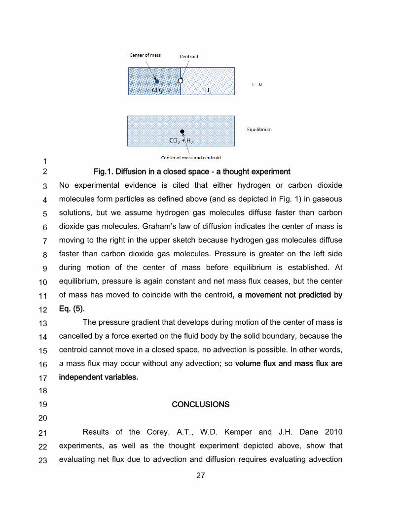
A thought experiment 16
The fact that net mass flux and advective flux are different variables, and 17
that Eq. (5) does not evaluate net mass flux is demonstrated by the following 18
thought experiment: Diffusion in a closed space is employed to illustrate that 19
even for this limiting condition, such that motion of reference volumes is 20
completely blocked, transport of mass by diffusion only is still possible. The 21
upper sketch depicts such a space where the center of mass of particles in the 22
space is moving to the right by diffusion. The bottom sketch of the same space 23
depicts the motion that has occurred after the center of mass has reached an 24
equilibrium position, so the center of mass and centroid coincide. 25
26
27
1
Fig.1. Diffusion in a closed space - a thought experiment 2
No experimental evidence is cited that either hydrogen or carbon dioxide 3
molecules form particles as defined above (and as depicted in Fig. 1) in gaseous 4
solutions, but we assume hydrogen gas molecules diffuse faster than carbon 5
dioxide gas molecules. Graham’s law of diffusion indicates the center of mass is 6
moving to the right in the upper sketch because hydrogen gas molecules diffuse 7
faster than carbon dioxide gas molecules. Pressure is greater on the left side 8
during motion of the center of mass before equilibrium is established. At 9
equilibrium, pressure is again constant and net mass flux ceases, but the center 10
of mass has moved to coincide with the centroid, a movement not predicted by 11
Eq. (5). 12
The pressure gradient that develops during motion of the center of mass is 13
cancelled by a force exerted on the fluid body by the solid boundary, because the 14
centroid cannot move in a closed space, no advection is possible. In other words, 15
a mass flux may occur without any advection; so volume flux and mass flux are 16
independent variables. 17
18
CONCLUSIONS 19
20
Results of the Corey, A.T., W.D. Kemper and J.H. Dane 2010 21
experiments, as well as the thought experiment depicted above, show that 22
evaluating net flux due to advection and diffusion requires evaluating advection 23
28
and diffusion independently. Eq. (5) does not evaluate mean flux if diffusion 1
occurs. A single flux equation to evaluate net flux where diffusion as well as 2
advection exists usually requires too many independent variables to be practical 3
for use in the general case where fluid particles with multiple masses are 4
involved. 5
The Corey, A.T., W.D. Kemper, and J.H. 2010 experiments show 6
advection of de-ionized liquid water is sometimes evaluated with acceptable 7
accuracy by Eq. (1) even where diffusion also is significant. These experiments 8
show self-diffusion of liquid water particles in a de-ionized solution is proportional 9
to the vapor pressure of a water solution. 10
Net flux of a particular particle in a water solution in porous media, in a 11
particular direction, is accomplished by first determining flux of the particle 12
associated with advection of the water solution as a whole in a particular 13
direction and adding the diffusive flux in that direction. 14
For a special case where advective flux is approximated with sufficient 15
accuracy by Eq. (1), an appropriate equation can be written as: 16
17
dx
dp
dx
dpK
c
cq i
vw
w
i
x iD
*
i (8) 18
19
For the particular case of flux of de-ionized liquid water, Eq. (8) reduces to: 20
21
dx
dp
dx
dpKq w
xxx
v
w
w
wwD
*
(9) 22
23
The driving forces in equations (8) and (9) are evaluated by directional 24
derivatives, not gradient operators. 25
Equations (8) and (9) apply to flux of water constituents in a de-ionized 26
liquid water solution where the water cluster is theoretically the only particle 27
transported by self-diffusion. Eq. (9) is verified by experimental evidence for net 28
29
flux of liquid water provided by Corey, A.T., W.D. Kemper and J.H. Dane 2010. 1
This equation can be applied to a special case of transport of water constituents 2
in liquid water solutions through porous media with channels small enough that 3
diffusion is significant, but large enough that Eq. (1) provides an adequate 4
evaluation of advection. 5
6
Need for additional research 7
Additional research is needed to evaluate flux of liquid solutions through 8
porous media, e.g., shale, compacted clay layers, or membranes that separate 9
living cells such as in capillaries in the mammalian cardiovascular or plant 10
systems. Research appearing in the literature to date does not show clearly 11
where transport of a reference volume is evaluated with sufficient accuracy by an 12
equation relating advective flux to the directional derivative of piezometric 13
pressure. A rule that describes conditions under which Eq. (1) evaluates 14
advective flux with acceptable accuracy is needed. 15
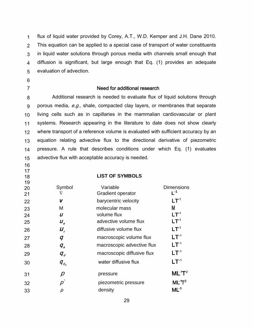
16 17 LIST OF SYMBOLS 18
19 Symbol Variable Dimensions 20 Gradient operator L-1
21
v barycentric velocity -1LT 22
M molecular mass M 23 u volume flux -1LT 24
au advective volume flux -1LT 25
d
u diffusive volume flux -1LT 26
q macroscopic volume flux -1LT 27
a
q macroscopic advective flux -1LT 28
dq macroscopic diffusive flux
-1LT 29
wd
q water diffusive flux -1LT 30
p pressure 2-1TML 31
*p piezometric pressure 2-1TML 32
ρ density -3ML 33
30
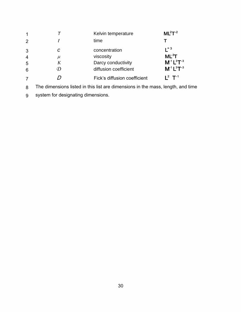
T Kelvin temperature -22TML 1
t time T 2
c concentration 3-L 3
viscosity TML-3 4 K Darcy conductivity
-33-1 TL M 5
D diffusion coefficient -33-1 TL M 6
D Fick’s diffusion coefficient 2L -1T 7
The dimensions listed in this list are dimensions in the mass, length, and time 8
system for designating dimensions. 9
31
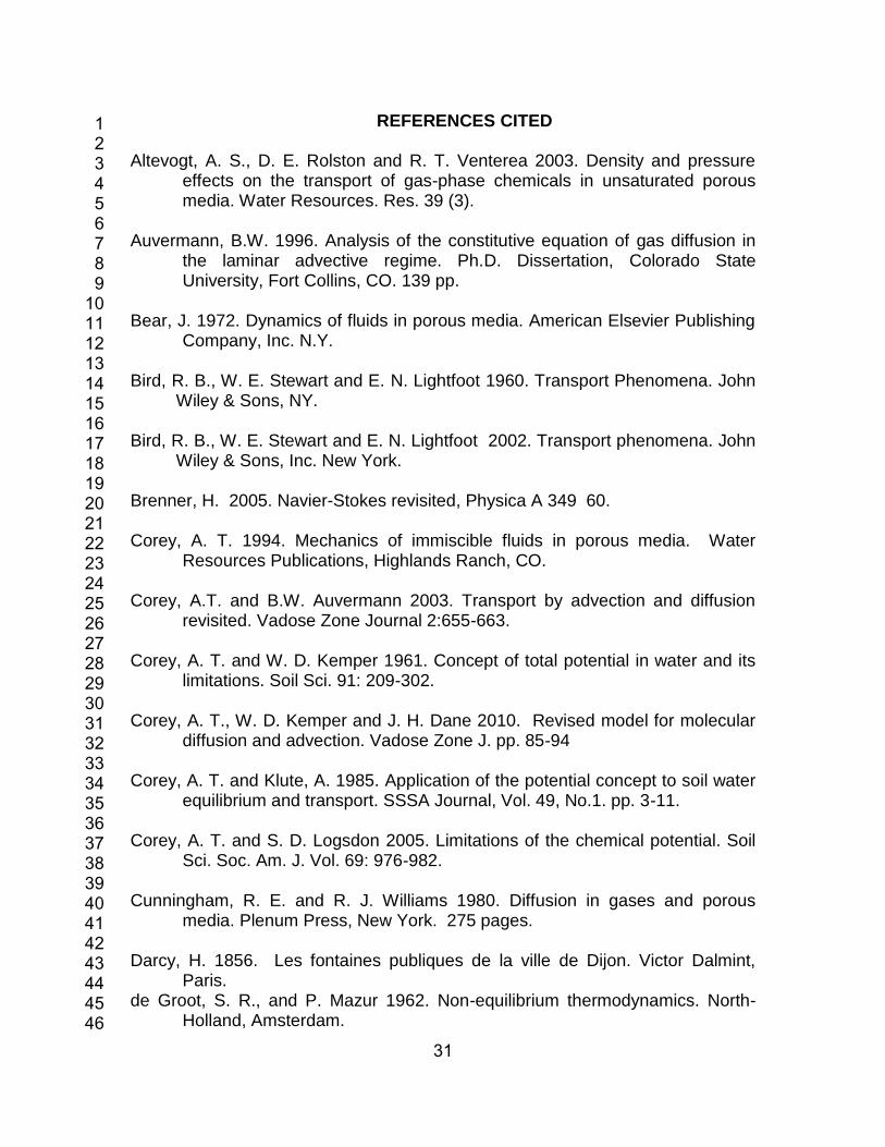
REFERENCES CITED 1 2 Altevogt, A. S., D. E. Rolston and R. T. Venterea 2003. Density and pressure 3
effects on the transport of gas-phase chemicals in unsaturated porous 4 media. Water Resources. Res. 39 (3). 5
6 Auvermann, B.W. 1996. Analysis of the constitutive equation of gas diffusion in 7
the laminar advective regime. Ph.D. Dissertation, Colorado State 8 University, Fort Collins, CO. 139 pp. 9
10 Bear, J. 1972. Dynamics of fluids in porous media. American Elsevier Publishing 11
Company, Inc. N.Y. 12 13 Bird, R. B., W. E. Stewart and E. N. Lightfoot 1960. Transport Phenomena. John 14
Wiley & Sons, NY. 15 16 Bird, R. B., W. E. Stewart and E. N. Lightfoot 2002. Transport phenomena. John 17
Wiley & Sons, Inc. New York. 18 19 Brenner, H. 2005. Navier-Stokes revisited, Physica A 349 60. 20 21 Corey, A. T. 1994. Mechanics of immiscible fluids in porous media. Water 22
Resources Publications, Highlands Ranch, CO. 23 24 Corey, A.T. and B.W. Auvermann 2003. Transport by advection and diffusion 25
revisited. Vadose Zone Journal 2:655-663. 26 27 Corey, A. T. and W. D. Kemper 1961. Concept of total potential in water and its 28
limitations. Soil Sci. 91: 209-302. 29 30 Corey, A. T., W. D. Kemper and J. H. Dane 2010. Revised model for molecular 31
diffusion and advection. Vadose Zone J. pp. 85-94 32 33 Corey, A. T. and Klute, A. 1985. Application of the potential concept to soil water 34
equilibrium and transport. SSSA Journal, Vol. 49, No.1. pp. 3-11. 35 36 Corey, A. T. and S. D. Logsdon 2005. Limitations of the chemical potential. Soil 37
Sci. Soc. Am. J. Vol. 69: 976-982. 38 39 Cunningham, R. E. and R. J. Williams 1980. Diffusion in gases and porous 40
media. Plenum Press, New York. 275 pages. 41 42 Darcy, H. 1856. Les fontaines publiques de la ville de Dijon. Victor Dalmint, 43
Paris. 44 de Groot, S. R., and P. Mazur 1962. Non-equilibrium thermodynamics. North-45
Holland, Amsterdam. 46
32
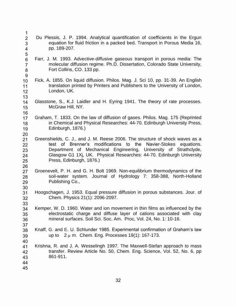
1 Du Plessis, J. P. 1994. Analytical quantification of coefficients in the Ergun 2
equation for fluid friction in a packed bed. Transport in Porous Media 16, 3 pp. 189-207. 4
5 Farr, J. M. 1993. Advective-diffusive gaseous transport in porous media: The 6
molecular diffusion regime. Ph.D. Dissertation, Colorado State University, 7 Fort Collins, CO. 133 pp. 8
9 Fick, A. 1855. On liquid diffusion. Philos. Mag. J. Sci 10, pp. 31-39. An English 10
translation printed by Printers and Publishers to the University of London, 11 London, UK. 12
13 Glasstone, S., K.J. Laidler and H. Eyring 1941. The theory of rate processes. 14
McGraw Hill, NY. 15 16 Graham, T. 1833. On the law of diffusion of gases. Philos. Mag. 175 (Reprinted 17
in Chemical and Physical Researches: 44-70. Edinburgh University Press, 18 Edinburgh, 1876.) 19
20 Greenshields, C. J., and J. M. Reese 2006. The structure of shock waves as a 21
test of Brenner’s modifications to the Navier-Stokes equations. 22 Department of Mechanical Engineering, University of Strathclyde, 23 Glasgow G1 1Xj, UK. Physical Researches: 44-70. Edinburgh University 24 Press, Edinburgh, 1876.) 25
26 Groenevelt, P. H. and G. H. Bolt 1969. Non-equilibrium thermodynamics of the 27
soil-water system. Journal of Hydrology 7: 358-388, North-Holland 28 Publishing Co., 29
30 Hoogschagen, J. 1953. Equal pressure diffusion in porous substances. Jour. of 31
Chem. Physics 21(1): 2096-2097. 32 33 Kemper, W. D. 1960. Water and ion movement in thin films as influenced by the 34
electrostatic charge and diffuse layer of cations associated with clay 35 mineral surfaces. Soil Sci. Soc. Am. Proc, Vol. 24, No. 1: 10-16. 36
37 Knaff, G. and E. U. Schlunder 1985. Experimental confirmation of Graham’s law 38
up to 2 m. Chem. Eng. Processes 19(1): 167-173. 39 40 Krishna, R. and J. A. Wesselingh 1997. The Maxwell-Stefan approach to mass 41
transfer. Review Article No. 50, Chem. Eng. Science, Vol. 52, No. 6, pp 42 861-911. 43
44 45

33
Malusis, M. A., C. H. Schackelford and H. W. Olsen 2001. A laboratory apparatus 1 to measure chemico-osmotic efficiency coefficients for clay soils. Geotech. 2 Test J. 24 (3):229-242. 3
4 Mason, E.A. and A. P. Malinauskas 1983. Gas transport in porous media: The 5
Dusty-Gas Model. Elsevier, Amsterdam-Oxford-New York. Vol 17. 6 7 Maxwell, J. C. 1866. On the dynamical theory of gases. Phil. Trans. R. Soc. 157: 8
49-88. 9 10 Olsen, H. W. 1985. Osmosis: A cause of apparent deviation from Darcy’s law. 11
Can. Geotech. J. 22: 238-241. 12 13 Streeter, V. L. 1948. Fluid Dynamics. McGraw–Hill Publications in Aeronautical 14
Science, NY. 15 16 Turner, J. S. 1973. Buoyancy affects in fluids. Cambridge University Press. 17 18 van’t Hoff, J. H. 1887. The role of osmotic pressure in the analogy between 19
solutions and gases. Z. Physik, Chemie 1: 481-493. A translation by 20 G.L. Blackshear. 21 22 Zemansky, M. W. and R. N. Dittman 1997. Heat and Thermodynamics. McGraw 23
Hill, NY. 24