Using a C1 triangular finite element based ona refined model for analyzing buckling andpost-buckling of multilayered plate/shell

structures

F. Dau∗ O. Polit∗∗ M.Touratier∗∗∗

∗LAMEFIP/ENSAM, Esplanade des arts et metiers, 33405 Talence-France∗∗LMpX, 1 Chemin Desvallieres, 92410 Ville d’Avray-France

∗∗∗LMSP-UMR CNRS-ENSAM/ESEM, 151 Bd de l’Hopital, 75013Paris-France

1 Introduction

Multilayered beam, plate and shell models and finite elements are needed in structuralmechanics for analyzing, dimensionning and designing this kind of structures. In the fieldof multilayered shells where transverse shear stress effects are of great importance, manyhigh order shell theories exist but very few numerical tools have been developped, see forexample the review paper [4].

The aim of this work is to present a new finite element, simple to use, free from classicalnumerical problems and very efficient for computing both displacements and stresses formultilayered shell applications. This new C1 shell finite element is based on the refinedkinematic model given in [7] which incorporates :

– a cosine distribution for the transverse shear strains avoiding the use of shear correc-tion factors,

– the continuity conditions between layers of the laminate for both displacements andtransverse shear stresses,

– the satisfaction of the boundary conditions at the top and bottom surfaces of theshell,

– the use of only five independent generalized displacements (three translations and tworotations).

A conforming finite element method and high-order finite element approximations, Ar-gyris interpolation for the transverse displacement and Ganev interpolation for membranedisplacements and transverse shear rotations, are both retained in this work.

Some unavoidable geometric shell considerations are firstly presented to introduce nec-essary tools for shell description. In the second part of this paper, the shell model basedon a refined kinematic approach is developped. The next part is dedicated to the finiteelement approximations and the present triangular finite element. Finally, numerical re-sults, compared with experimental ones, are presented. Good results on classical tests for

1

multilayered plates and shells for both linear static and dynamic analysis have already beenobtained using this new element. In this paper, critical buckling and post buckling prob-lems are especially studied to show the efficiency of this new finite element for multilayeredstructures.

2 Geometric considerations

A shell C with a middle surface S and a constant thickness e is defined by, see [3] :

C =M ∈ R3 :

−−→OM(ξ, ξ3) = ~Φ(ξ) + ξ3~a3; ξ ∈ Ω;−1

2e(ξ) ≤ ξ3 ≤ 1

2e(ξ)

where the middle surface is described by a map ~Φ from a parametric bidimensional domainΩ as :

~Φ : Ω ⊂ R2 −→ S ⊂ R3

ξ = (ξ1, ξ2) 7−→ ~Φ(ξ)(1)

For a point on the shell middle surface, covariant base vectors are usually obtained asfollows :

~aα = ~Φ(ξ1, ξ2),α ; ~a3 =~a1 × ~a2

||~a1 × ~a2||= ~t3 (2)

In Eq. (2) and further on, latin indices i, j, . . . take their values in the set 1, 2, 3 whilegreek indices α, β, . . . take their values in the set 1, 2. The summation convention on

repeated indices and the classic notation ( ),α =∂( )

∂ξαare used.

For any point of the shell, covariant base vectors are now deduced as :

~gα = ~r(ξ1, ξ2, ξ3),α = (δβα − ξ3bβα)~aβ = µβα~aβ and ~g3 = ~a3 (3)

The mixed tensor mβα must also be introduced and is defined by the relation :

mβα = (µ−1)βα =

1

µδβα + ξ3(bβα − 2Hδβα) (4)

where µ = det(µβα) = 1− 2Hξ3 + (ξ3)2K ; H = 12tr(bβα) ; K = det(bβα).

Therefore, the covariant metric tensor aαβ, covariant bαβ and mixte bβα curvature tensorscan be defined. These tensors and some relations between them are recalled hereafter :

aαβ = aβα = ~aα.~aβ

bαβ = bβα = −~aα.~a3,β

~aα = aαβ~aβ

bβα = aβγbγαa = det(aαβ) (5)

Finally, the surface element dS and the volume element dV are classically given by :

dS =√adξ1dξ2

dV = µdSdξ3 (6)

All these relations are classic and more details in order to obtain the Christoffel symbolsand other differential geometric entities could be found in Bernadou [3].

2

3 The shell model

3.1 The displacement field

Let us denote by u(k)i (ξ1, ξ2, ξ3 = z, t), i ∈ 1, 2, 3 the curvilinear components of the

displacement field associated with the contravariant base vectors ~ai.The refined displacement field is based on continuity requierements from [2] and follows

classical plate/shell assumption σ33 = 0. In a layer (k), it is expressed as [5] :

u(k)1 (ξ1, ξ2, z, t) = µα1 vα(ξ1, ξ2, t)− z v3,1(ξ1, ξ2, t) + F α

1(k)(z) γ0

α(ξ1, ξ2, t)

u(k)2 (ξ1, ξ2, z, t) = µα2 vα(ξ1, ξ2, t)− z v3,2(ξ1, ξ2, t) + F α

2(k)(z) γ0

α(ξ1, ξ2, t)

u(k)3 (ξ1, ξ2, z, t) = v3(ξ1, ξ2, t)

(7)

where t is the time and the classical summation on repeated indices is used. In Eq. (7),vi are displacements of a point on the middle surface and γ0

α is the transverse shear strainat z = 0, while F α

β(k) are functions of the normal transverse co-ordinate z defining the

distribution of the transverse shear stresses through the thickness. They are defined by :

F 11

(k)(z) = f1(z) + g1(k)(z) F 2

1(k)(z) = g2

(k)(z)F 1

2(k)(z) = g3

(k)(z) F 22

(k)(z) = f2(z) + g4(k)(z)

(8)

In Eq. (8), the thickness functions f1, f2, g1(k), . . . , g4

(k) depend on coefficients a(k)i , d

(k)i , b44, b55

and trigonometric functions as follows :

f1(z) = f(z)− eπb55f

′(z)f2(z) = f(z)− e

πb44f

′(z)gi

(k)(z) = ai(k)z + di

(k) i = 1, 2, 3, 4. and k = 1, 2, 3, . . . , N.(9)

with f(z) =e

πsin

πz

eand f ′(z) stands for f(z) derivative with respect to z co-ordinate. N

represents the number of layers.

These coefficients are determined from the boundary conditions on the top and bot-tom surfaces of the shell, and from the continuity requirements at the layer interfaces fordisplacements and stresses, see Beakou [2].

From Eq. (7), classical shell models can be deduced :

• the classical shell theory (Koıter theory), called CST model with :

f1(z) = f2(z) = 0 et gki (z) = 0

• the first order shear deformation theory (Naghdi theory), called FSDT model with :

f1(z) = f2(z) = z et gki (z) = 0

Hereafter, the superscript (k) for uα(k) components is omitted in order to simplify the finite

element description.

3

3.2 The strain field

After some algebraic calculations, the covariant strain tensor components are obtained inthe local contravariant basis ~ai as follows :

ε = εij(ai ⊗ aj) with

2εαβ =1

µ

(ε0αβ + ε0βα + F ν

α (z) ε1νβ + F νβ (z) ε1να +Gν

α(z) ε2νβ +Gνβ(z) ε2να

+z

(bλβ − 2Hδλβ) (ε0αλ + F να (z) ε1νλ +Gν

α(z) ε2νλ) +

(bλα − 2Hδλα)(ε0βλ + F ν

β (z) ε1νλ +Gνβ(z) ε2νλ

))

2εα3 = F ν′α (z) γ0

ν

(10)

with Gνα(z) = F ν

α (z) − δνα z and F ν′α (z) stands for F ν

α (z) derivative with respect to z co-ordinate.

By convenience, the following notations have been introduced in Eq. (10) to caracterizethe mechanical effects :

membrane strain : ε0αβ = vα|β − bαβv3

bending strain 1 : ε1αβ = βα|β

bending strain 2 : ε2αβ = bλαvλ|β + bλα|βvλ + v3|αβ

transverse shear strain : γ0α = βα + bβαvβ + v3,α

where the notation |β stands for the covariant derivation with respect to the ξβ curvilinearco-ordinate.

4 The finite element approximation

4.1 The discrete weak form of the boundary value problem

The discrete formulation of the shell boundary value problem in linear elasticity is deducedfrom the following functional :

a(~uh, ~u∗h)∪Ωe = f(~u∗h)∪Ωe + F (~u∗h)∪Ce , ∀~u∗h (11)

where ∪Ωe is the triangulation of the multilayered structure and ∪Ce is the edge of themeshed structure. In addition, ~uh is the finite element approximation of the displacementfield ~u given by Eq. (7) and ~u∗h is the finite element approximation of the correspondingvirtual velocity field ~u∗. Linear functions f and F represent the body (including inertiaterms) and surface loads, actually surface and line loads respectively, due to the integrationperformed throughout the thickness in Eq. (11). The superscript h introduced in Eq. (11)indicates the finite element approximation. It is also used for finite element approximationof the generalized displacements in Eq. (7), denoted by vi

h and θαh with i = 1, 2, 3 and

α = 1, 2.The geometry of the shell is approximated by the classical three node triangular finite

element.

4

4.2 The generalized displacement approximations

In a conforming finite element approach, the displacement field, given by Eq. (7) indicatesthat v3

h must be approximated by a C1-continuous function. The other generalized dis-placements vα

h and θαh have to be defined in the Sobolev space H1(Ωe). Those functions

must be at least C0-continuous.Therefore, Argyris interpolation for the deflexion and the Ganev interpolation for the

other generalized displacements are used. Note that the Argyris interpolation is exactlyof continuity C1 and the Ganev interpolation involves a semi-C1 continuity which is notneeded here. Due to very long expressions for these interpolations, the reader is referred toeither the original papers [1] and [6] or a recent book [3].

The degrees of freedom associated with one finite element in the local curvilinear basisare given as :

• for a corner node :v1 v1,1 v1,2 v2 v2,1 v2,2

v3 v3,1 v3,2 v3,11 v3,22 v3,12

θ1 θ1,1 θ1,2 θ2 θ2,1 θ2,2

(12)

• while, for a mid-side node :v1 v1,n v2 v2,n

v3,n

θ1 θ1,n θ2 θ2,n

(13)

where p,n is the derivative with respect to the normal direction of the edge element.

Then, having derivatives in the previous set of degrees of freedom (dof), the followingmethodology is used to prescribe kinematic boundary conditions.

For a given p function with the condition p(ξ1 = 0, ξ2) = 0 to satisfy ∀ξ2, then the firstorder derivatives become :

p,1(0, ξ2) = limh→0p(h, ξ2)− p(0, ξ2)

h6= 0

p,2(0, ξ2) = limh→0p(0, ξ2 + h)− p(0, ξ2)

h= 0

(14)

and so on for the second order derivatives.

4.3 The elementary matrices

4.3.1 The stiffness matrix

The elementary stiffness matrix [Ke] is obtained by computing the bilinear form given inEq. (11) at the elementary level as :

a(~uh, ~u∗h)Ωe =∫

Ωe

∫ e/2

−e/2

[ε∗eh]T [

C(k)] [εeh]µdz√adΩe

=∫

Ωe

[E∗e

h]T(∫ e/2

−e/2[Be]

T[C(k)

][Be]µdz

) [Ee

h]√

adΩe

=∫

Ωe

[E∗e

h]T

[Ae][Ee

h]√

adΩe

= [Q∗e]T [Ke] [Qe]

(15)

5

Using the displacement field ~u in Eq. (7) and the strain components in Eq. (10), thematrix [Be] can easily be deduced. It is computed by the following relation :

[Be] = [Ep][Geo] (16)

In the above expression of matrix [Be], [Ep] is a matrix containing thickness functionsof the co-ordinate z whereas [Geo] is a matrix including only differential geometry entitiessuch as metric tensor, curvature tensor and Christoffel symbols (see Bernadou [3]).

The matrix [Eeh] (identically for [E∗e

h] adding the asterisk superscript), which may beseen as a generalized displacements matrix, is given by :

[Ee

h]T

=[v1h v1

h,1 v1

h,2

... v2h v2

h,1 v2

h,2

...

v3h v3

h,1 v3

h,2 v3

h,11 v3

h,12 v3

h,22

...

θ1h θ1

h,1 θ1

h,2

... θ2h θ2

h,1 θ2

h,2

](17)

The finite element approximations, defined at the above section 4.2, are directly usedto express the matrix

[Ee

h]

as a function of the elementary degrees of freedom vector [Qe]

(see Eq. (12) and Eq. (13)).Finally, [Ae] contains the material behaviour matrix for a multilayered finite element,

resulting from the integration with respect to the thickness co-ordinate, and differentialgeometry entities such as metric, curvature, Christoffel symbols, . . .

4.4 Extension to the geometric non linearity

The multilayered structure is now considered in a Total Lagrangian configuration, so that itsmesh is denoted ∪Ωe(0) with edge ∪Ce(0) where (0) indicates the initial (fixed) configurationused. Lagrangian co-ordinates will hereafter be written ξi as previously. The discreteboundary value problem ”stated” above for linear analysis Eq. (11) is therefore formulatedby the following Total Lagrangian functional available for non-linear analysis :

J(~uh, ~u∗h)∪Ωe(0) = a(~uh, ~u∗h)∪Ωe(0) − f(~u∗h)∪Ωe(0) − F (~u∗h)∪Ce(0) = 0 , ∀~u∗h (18)

Absence of followed forces is considered here. Thus, the main feature of the non-linearformulation is incorporated into the virtual internal power and the following expression isobtained :

a(~uh, ~u∗h)Ω(0) =∫

Ω(0)

∫ e/2

−e/2

[ε∗eh]T [

C(k)] [εeh]µdz√adΩe(0) (19)

All the quantities in Eq. (19) refer to the initial (fixed) configuration. Virtual strainrates and strains can be split into their linear (index L) and non-linear (index NL) partsas follows : [

ε∗eh]

=[εL∗eh]

+[εNL

∗eh]

[εeh]

=[εLe

h]

+[εNLe

h] (20)

The geometrically non-linear formulation now considered is based on Von-Karmannassumptions where deflexion is moderately large, while rotations and strains remain small.Non-linear virtual strain rate matrix in Eq. (20) is then given by :

[εNL

∗eh]T

= [1

2(v3

h,1 + bα1 vα

h)(v∗3h,1 + bα1 v

∗αh)

1

2(v3

h,2 + bα2 vα

h)(v∗3h,2 + bα2 v

∗αh)

(v3h,1 + bα1 vα

h)(v∗3h,2 + bλ2v

∗λh) + (v3

h,2 + bα2 vα

h)(v∗3h,1 + bλ1v

∗λh)

0 0 ]

(21)

6

and non-linear strain matrix is :

[εNLe

h]T

= [1

2(v3

h,1 + bα1 vα

h)2 1

2(v3

h,2 + bα2 vα

h)2

(v3h,1 + bα1 vα

h)(v3h,2 + bλ2vλ

h) 0 0 ](22)

4.4.1 Consistent linearization procedure

From these last equations, it is evident that Eq. (19) is non-linear with respect to displace-ments, and a Newton algorithm has to be used to find a numerical solution of Eq. (18). Fora Newton-type method, knowledge of the tangent stiffness is required and can be derivedusing standard linearization procedures. Applying it to Eq. (18), we obtain :

J(~uh, ~u∗h)∪Ωe(0) = J(~uh, ~u∗h)∪Ωe(0) +D~uJ(~u

h, ~u∗h).∆~uh (23)

with ~uh = ~uh

+ ∆~uh, where ~uh

refers to a known state.According to Eq. (23), the linearized form of the functional Eq. (18) is deduced and we

now have to find the solution of the following equation :

D~ua(~uh, ~u∗h)∪Ωe(0).∆~u

h = −a(~uh, ~u∗h)∪Ωe(0) + f(~u∗h)∪Ωe(0) + F (~u∗h)∪Ce(0) , ∀~u∗h (24)

The left member of Eq. (24) has to be computed and gives the tangent operator, whileother quantities in the right member are known vectors as they depend only on the known

state ~uh.

4.4.2 The tangent stiffness matrix

The tangent stiffness matrix is now derived from the left member of Eq. (24). For anarbitrary finite element Ωe(0) of the mesh ∪Ωe(0), the tangent operator is found as :

D~ua(~uh, ~u∗h)Ωe(0).∆~u

h =∫

Ωe(0)

[E∗e

h]T

[Ae][∆Ee

h]√

adΩe(0)+∫

Ωe(0)

[E∗e

h]T [

Ae(~uh)] [

∆Eeh]√

adΩe(0)+∫

Ωe(0)

[E∗e

h]T [

Ae(σh)] [

∆Eeh]√

adΩe(0)

(25)

In Eq. (25), the matrix [Ae] has been given in 4.3.1 (see Eq. (15)), as well as vectors

[Eeh] and [∆Ee

h] = ∆[Eeh] from Eq. (17). The matrix [Ae(~u

h)] depends on material

properties and on both linear and quadratic known state ~uh. Finally, the matrix [Ae(σ

h)]is linked to the in-plane stresses.

Following the procedure given in 4.3.1 to derive the linear stiffness matrix [Ke], it iseasy to compute the tangent stiffness matrix, denoted [KT e], so that :

D~ua(~uh, ~u∗h)Ωe(0).∆~u

h = [Q∗e]T [KT e] [∆Qe] (26)

where[KT e] = [Ke] +

[Ke(~u

h)]

+[Ke(σ

h)]

(27)

In Eq. (27), to compute either matrix [Ke] or[Ke(~u

h)]

or[Ke(σ

h)], we use Eq. (15)

respectively based either on [Ae] or [Ae(~uh)] or [Ae(σ

h)].

7

5 Numerical results on non linear test

Only buckling and post-buckling analysis are presented here. For both analysis, numericalsimulations are compared with results issued from experiments. Experiment and modelisa-tion are firstly described and results are then discussed.

Experiment : Experimental conditions are now described.

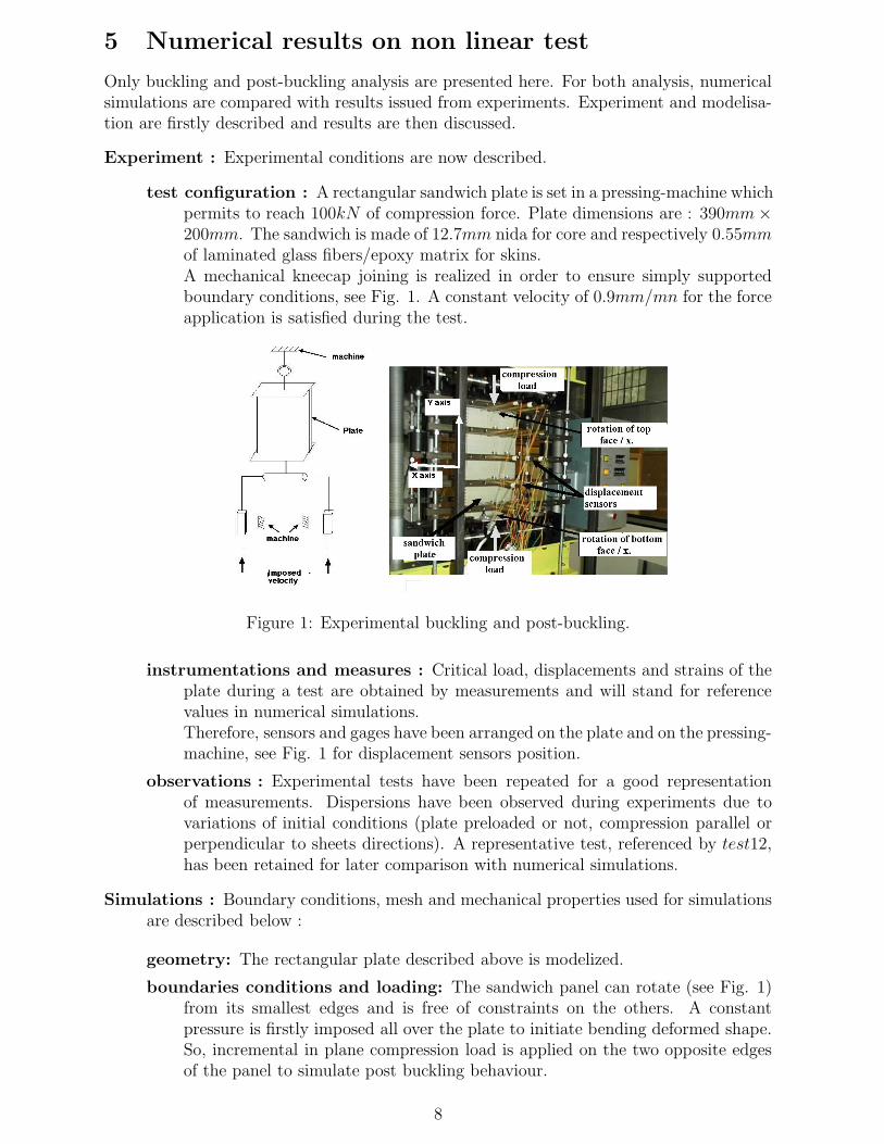
test configuration : A rectangular sandwich plate is set in a pressing-machine whichpermits to reach 100kN of compression force. Plate dimensions are : 390mm×200mm. The sandwich is made of 12.7mm nida for core and respectively 0.55mmof laminated glass fibers/epoxy matrix for skins.A mechanical kneecap joining is realized in order to ensure simply supportedboundary conditions, see Fig. 1. A constant velocity of 0.9mm/mn for the forceapplication is satisfied during the test.

Figure 1: Experimental buckling and post-buckling.

instrumentations and measures : Critical load, displacements and strains of theplate during a test are obtained by measurements and will stand for referencevalues in numerical simulations.Therefore, sensors and gages have been arranged on the plate and on the pressing-machine, see Fig. 1 for displacement sensors position.

observations : Experimental tests have been repeated for a good representationof measurements. Dispersions have been observed during experiments due tovariations of initial conditions (plate preloaded or not, compression parallel orperpendicular to sheets directions). A representative test, referenced by test12,has been retained for later comparison with numerical simulations.

Simulations : Boundary conditions, mesh and mechanical properties used for simulationsare described below :

geometry: The rectangular plate described above is modelized.

boundaries conditions and loading: The sandwich panel can rotate (see Fig. 1)from its smallest edges and is free of constraints on the others. A constantpressure is firstly imposed all over the plate to initiate bending deformed shape.So, incremental in plane compression load is applied on the two opposite edgesof the panel to simulate post buckling behaviour.

8

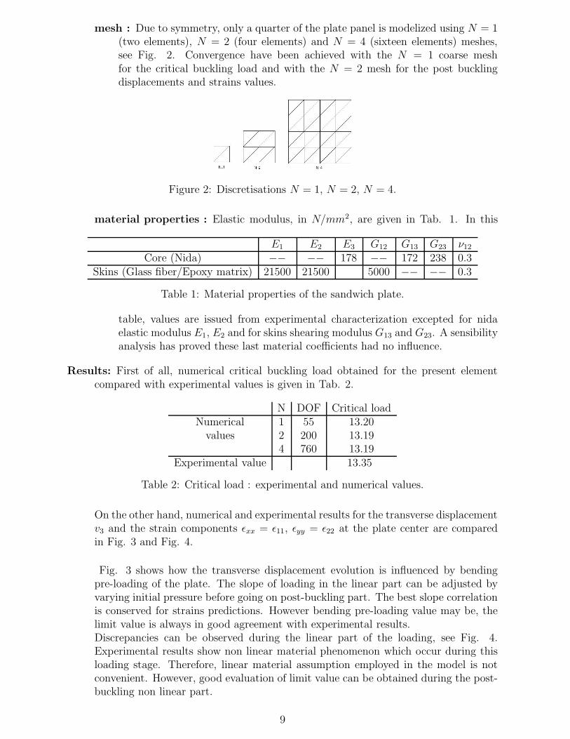
mesh : Due to symmetry, only a quarter of the plate panel is modelized using N = 1(two elements), N = 2 (four elements) and N = 4 (sixteen elements) meshes,see Fig. 2. Convergence have been achieved with the N = 1 coarse meshfor the critical buckling load and with the N = 2 mesh for the post bucklingdisplacements and strains values.

Figure 2: Discretisations N = 1, N = 2, N = 4.

material properties : Elastic modulus, in N/mm2, are given in Tab. 1. In this

E1 E2 E3 G12 G13 G23 ν12

Core (Nida) −− −− 178 −− 172 238 0.3Skins (Glass fiber/Epoxy matrix) 21500 21500 5000 −− −− 0.3

Table 1: Material properties of the sandwich plate.

table, values are issued from experimental characterization excepted for nidaelastic modulus E1, E2 and for skins shearing modulus G13 and G23. A sensibilityanalysis has proved these last material coefficients had no influence.

Results: First of all, numerical critical buckling load obtained for the present elementcompared with experimental values is given in Tab. 2.

N DOF Critical loadNumerical 1 55 13.20

values 2 200 13.194 760 13.19

Experimental value 13.35

Table 2: Critical load : experimental and numerical values.

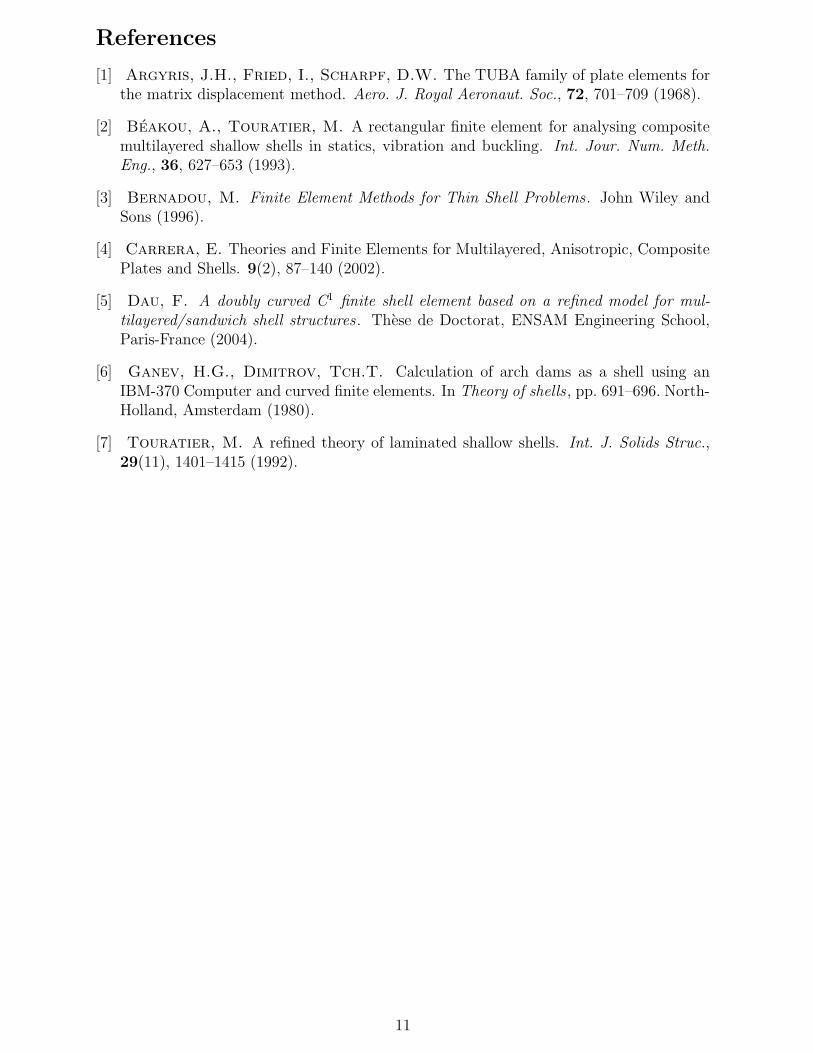
On the other hand, numerical and experimental results for the transverse displacementv3 and the strain components εxx = ε11, εyy = ε22 at the plate center are comparedin Fig. 3 and Fig. 4.

Fig. 3 shows how the transverse displacement evolution is influenced by bendingpre-loading of the plate. The slope of loading in the linear part can be adjusted byvarying initial pressure before going on post-buckling part. The best slope correlationis conserved for strains predictions. However bending pre-loading value may be, thelimit value is always in good agreement with experimental results.Discrepancies can be observed during the linear part of the loading, see Fig. 4.Experimental results show non linear material phenomenon which occur during thisloading stage. Therefore, linear material assumption employed in the model is notconvenient. However, good evaluation of limit value can be obtained during the post-buckling non linear part.

9

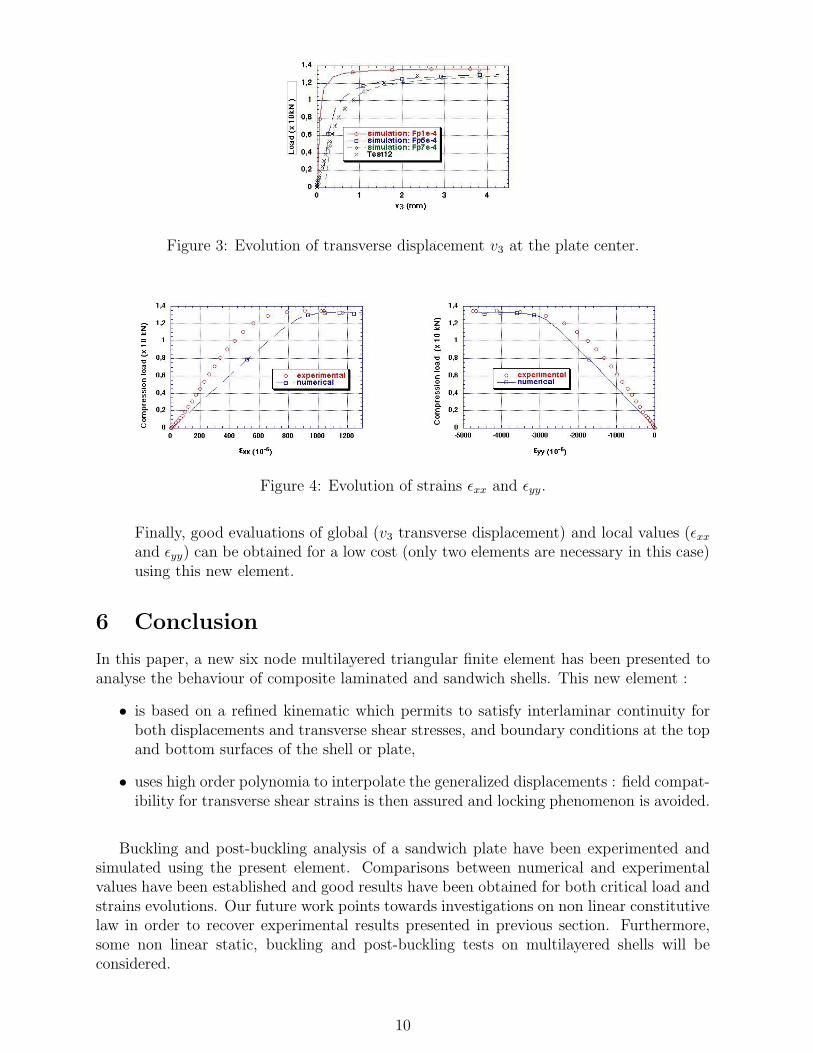
Figure 3: Evolution of transverse displacement v3 at the plate center.

Figure 4: Evolution of strains εxx and εyy.

Finally, good evaluations of global (v3 transverse displacement) and local values (εxxand εyy) can be obtained for a low cost (only two elements are necessary in this case)using this new element.

6 Conclusion

In this paper, a new six node multilayered triangular finite element has been presented toanalyse the behaviour of composite laminated and sandwich shells. This new element :

• is based on a refined kinematic which permits to satisfy interlaminar continuity forboth displacements and transverse shear stresses, and boundary conditions at the topand bottom surfaces of the shell or plate,

• uses high order polynomia to interpolate the generalized displacements : field compat-ibility for transverse shear strains is then assured and locking phenomenon is avoided.

Buckling and post-buckling analysis of a sandwich plate have been experimented andsimulated using the present element. Comparisons between numerical and experimentalvalues have been established and good results have been obtained for both critical load andstrains evolutions. Our future work points towards investigations on non linear constitutivelaw in order to recover experimental results presented in previous section. Furthermore,some non linear static, buckling and post-buckling tests on multilayered shells will beconsidered.

10

References

[1] Argyris, J.H., Fried, I., Scharpf, D.W. The TUBA family of plate elements forthe matrix displacement method. Aero. J. Royal Aeronaut. Soc., 72, 701–709 (1968).

[2] Beakou, A., Touratier, M. A rectangular finite element for analysing compositemultilayered shallow shells in statics, vibration and buckling. Int. Jour. Num. Meth.Eng., 36, 627–653 (1993).

[3] Bernadou, M. Finite Element Methods for Thin Shell Problems. John Wiley andSons (1996).

[4] Carrera, E. Theories and Finite Elements for Multilayered, Anisotropic, CompositePlates and Shells. 9(2), 87–140 (2002).

[5] Dau, F. A doubly curved C1 finite shell element based on a refined model for mul-tilayered/sandwich shell structures. These de Doctorat, ENSAM Engineering School,Paris-France (2004).

[6] Ganev, H.G., Dimitrov, Tch.T. Calculation of arch dams as a shell using anIBM-370 Computer and curved finite elements. In Theory of shells, pp. 691–696. North-Holland, Amsterdam (1980).

[7] Touratier, M. A refined theory of laminated shallow shells. Int. J. Solids Struc.,29(11), 1401–1415 (1992).

11