Embed Size (px)
Citation preview
1
Visualization and Data Mining techniques
By- Group number- 14
Chidroop Madhavarapu(105644921)Deepanshu Sandhuria(105595184)
Data Mining CSE 634Prof. Anita Wasilewska
2
References
http://coblitz.codeen.org:3125/citeseer.ist.psu.edu/cache/papers/cs/10335/ftp:zSzzSzftp.cs.umn.eduzSzdeptzSzuserszSzkumarzSzdatavis.pdf/ganesh96visual.pdf
http://www.ailab.si/blaz/predavanja/ozp/gradivo/2002-Keim-Visualization%20in%20DM-IEEE%20Trans%20Vis.pdf
http://www.geocities.com/anand_palm/
http://citeseer.ist.psu.edu/cache/papers/cs/27216/http:zSzzSzwww-users.cs.umn.eduzSzzCz7EctluzSzPaperTalkFilezSzits02.pdf/shekhar02cubeview.pdf
http://www.cs.umn.edu/Research/shashi-group/
http://www.cs.umn.edu/Research/shashi-group/Book/sdb-chap1.pdf
http://www.cs.umn.edu/research/shashi-group/alan_planb.pdf
http://coblitz.codeen.org:3125/citeseer.ist.psu.edu/cache/papers/cs/27637/http:zSzzSzwww-users.cs.umn.eduzSzzCz7EpushengzSzpubzSzkdd2001zSzkdd.pdf/shekhar01detecting.pdf

3
Motivation
Visualization for Data Mining
• Huge amounts of information
• Limited display capacity of output devices
Visual Data Mining (VDM) is a new approach forexploring very large data sets, combining traditionalmining methods and information visualization
techniques.

4
Why Visual Data Mining

5
Why Visual Data Mining
6
VDM Approach
VDM takes advantage of both,
The power of automatic calculations, and
The capabilities of human processing. Human perception offers phenomenal
abilities to extract structures from pictures.

7
Levels of VDM
No or very limited integration Corresponds to the application of either traditional
information visualization or automated data mining methods.
Loose integration Visualization and automated mining methods are applied
sequentially.
The result of one step can be used as input for another step.
Full integration Automated mining and visualization methods applied in
parallel.
Combination of the results.
8
Methods of Data Visualization
Different methods are available for visualization of data
based on type of data
Data can be
Univariate
Bivariate
Multivariate

9
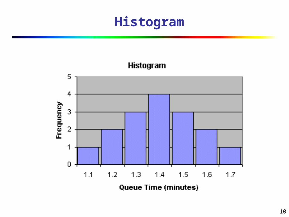
Univariate data
Measurement of single quantitative variable
Characterize distribution
Represented using following methods
Histogram
Pie Chart
10
Histogram

11
Pie Chart

12
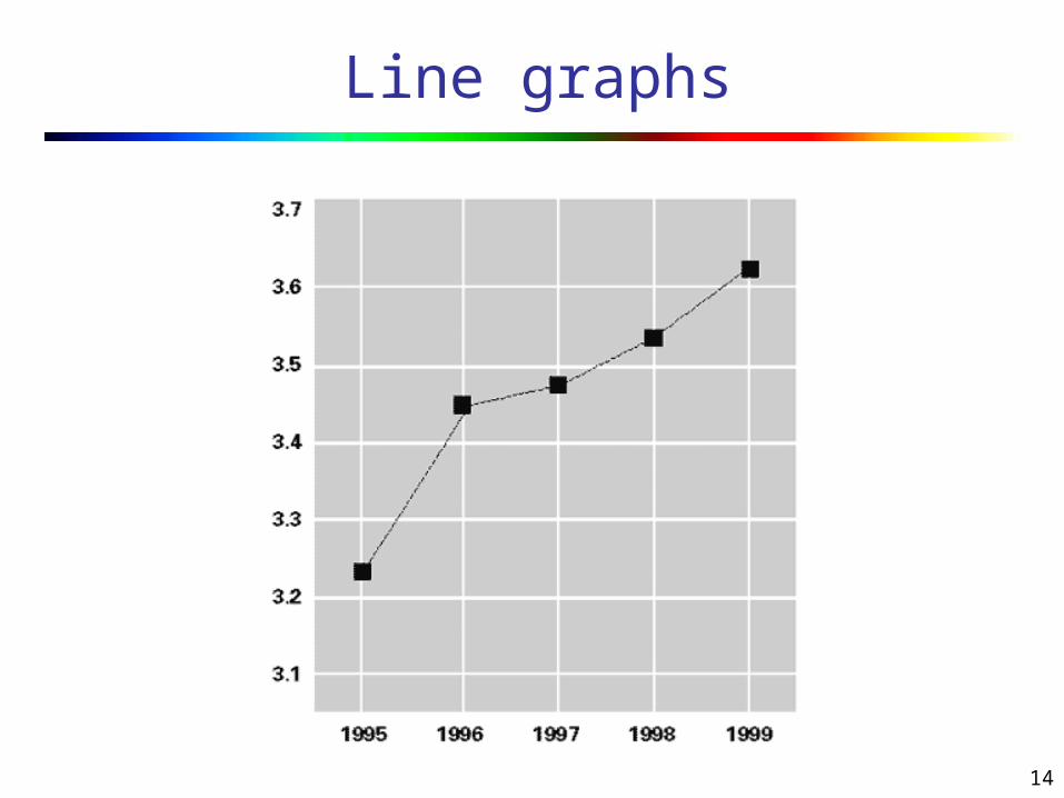
Bivariate Data
Constitutes of paired samples of two quantitative variables
Variables are related
Represented using following methods
Scatter plots
Line graphs

13
Scatter plots
14
Line graphs

15
Multivariate Data
Multi dimensional representation of multivariate data
Represented using following methods
Icon based methods
Pixel based methods
Dynamic parallel coordinate system

16
Icon based Methods
17
Pixel Based Methods
Approach:
Each attribute value is represented by one colored pixel (the value ranges of the attributes are mapped to a fixed color map).
The values of each attribute are presented in separate sub windows.
Examples: Dense Pixel Displays
18
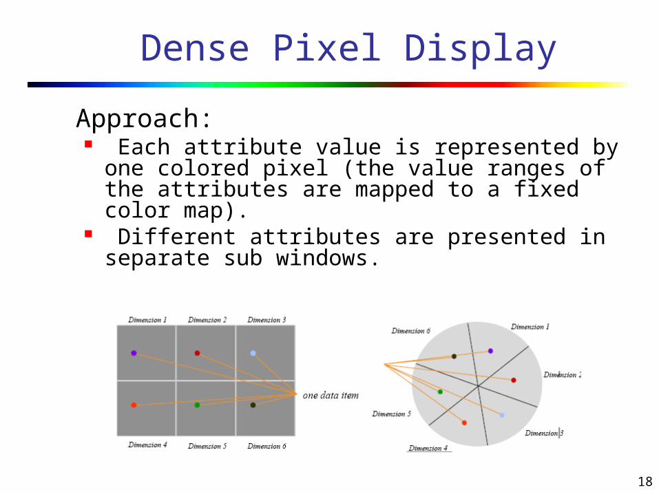
Dense Pixel Display
Approach: Each attribute value is represented by one
colored pixel (the value ranges of the attributes are mapped to a fixed color map).
Different attributes are presented in separate sub windows.
19
Visual Data Mining: Framework and Algorithm Development
Ganesh, M., Han, E.H., Kumar, V., Shekar, S., & Srivastava, J. (1996).
Working Paper. Twin Cities, MN: University of Minnesota, Twin Cities Campus.

20
References
http://coblitz.codeen.org:3125/citeseer.ist.psu.edu/cache/papers/cs/10335/ftp:zSzzSzftp.cs.umn.eduzSzdeptzSzuserszSzkumarzSzdatavis.pdf/ganesh96visual.pdf
http://www.ailab.si/blaz/predavanja/ozp/gradivo/2002-Keim-Visualization%20in%20DM-IEEE%20Trans%20Vis.pdf
http://www.geocities.com/anand_palm/
21
Abstract
VDM refers to refers to the use of visualization techniques in Data Mining process to
Evaluate Monitor Guide
This paper provides a framework for VDM via the loose coupling of databases and visualization systems.
The paper applies VDM towards designing new algorithms that can learn decision trees by manually refining some of the decisions made by well known algorithms such as C4.5.

22
Components of VQLBCI
The three major components of VQLBCI are Visual Representations, Computations and Events.

23
Visual Development of Algorithms
Most interesting use of visual data mining is the development of new insights and algorithms.
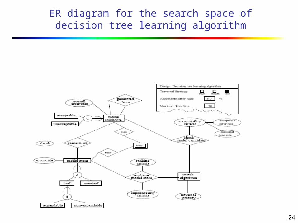
The figure below shows the ER diagram for learning classification decision trees.
This model allows the user to monitor the quality and impact of decisions made by the learning procedure.
Learning procedure can be refined interactively via a visual interface.
24
ER diagram for the search space of decision tree learning algorithm
25
General Framework
Learning a classification decision tree from a training data set can be regarded as a process of searching for the best decision tree that meets user-provided goal constraints.
The problem space of this search process consists of Model Candidates, Model Candidate Generator and Model Constraints.
Many existing classification-learning algorithms like C4.5 and CDP fit nicely within this search framework. New learning algorithms that fit user’s requirements can be developed by defining the components of the problem space.

26
General Framework
Model Candidate corresponds to the partial classification decision tree. Each node of the decision tree is a Model Atom
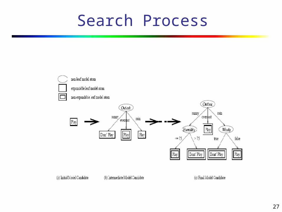
Search process is the process of finding a final model candidate such that it meets user goal specifications.
Model Candidate Generator transforms the current model candidate into a new model candidate by selecting one model atom to expand from the expandable leaf model atoms.
Model Constraints (used by Model Candidate Generator) provide controls and boundaries to the search space.
27
Search Process

28
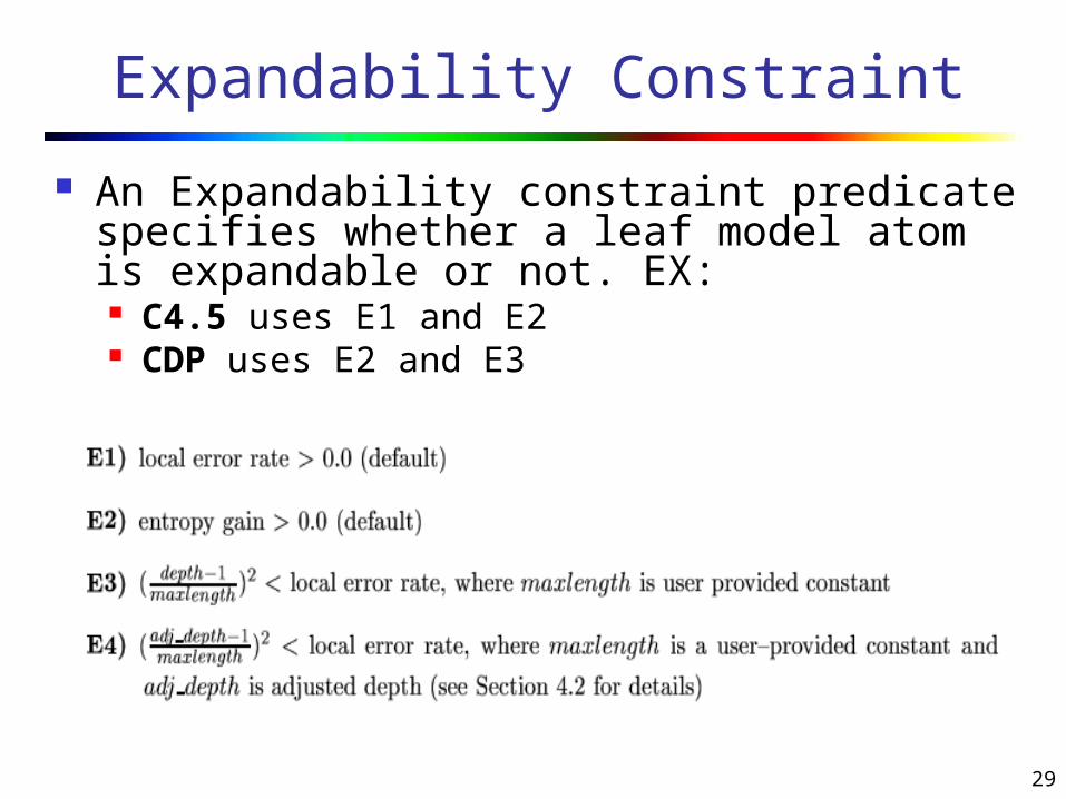
Acceptability Constraint
Model Constraints consist of Acceptability constraints, Expandability constraints and a Data-Entropy calculation function.
Acceptability constraint predicate specifies when a model candidate is acceptable and thus allows search process to stop. EX:
A1) Total no of expandable leaf model atoms = 0. A2) Overall error rate of the model candidate <=
acceptable error rate. A3) Total number of model atoms in the model
candidate>= maximal allowable tree size.
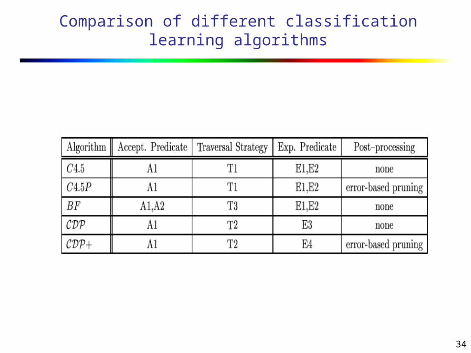
A1 is used in C4.5 and CDP
29
Expandability Constraint
An Expandability constraint predicate specifies whether a leaf model atom is expandable or not. EX: C4.5 uses E1 and E2 CDP uses E2 and E3
30
Traversal Strategy
Traversal strategy ranks expandable leaf model atoms based on the model atom attributes. EX:
Increasing order of depth Decreasing order of depth Orders based on other model atom attributes.

31
Steps in Visual Algorithm Development
No single algorithm is the best all the time, performance is highly data dependent.
By changing different predicates of model constraints, users can construct new classification-learning algorithm.
This enables users to find an algorithm that works the best on a given data set.
Two algorithms are developed : BF based on Best First search idea and CDP+ which is a modification of CDP
32
BF
This algorithm is based on the Best-First search idea.
For Acceptability criteria, it includes A1 and A2 with a user specified acceptable error rate.
The Traversal strategy chosen is T3 In Best-First, expandable leaf model atoms
are ranked according to the decreasing order of the number of misclassified training cases. (local error rate * size of subset training data set)
The traversal strategy will expand a model atom that has the most misclassified training cases, thus reducing the overall error rate the most.
33
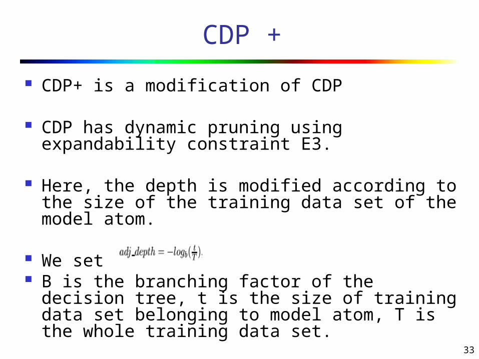
CDP +
CDP+ is a modification of CDP
CDP has dynamic pruning using expandability constraint E3.
Here, the depth is modified according to the size of the training data set of the model atom.
We set B is the branching factor of the decision tree,
t is the size of training data set belonging to model atom, T is the whole training data set.
34
Comparison of different classification learning algorithms
35
Experiment
The new BF and CDP+ algorithms are compared with the C4.5 and CDP algorithms.
Various metrics are selected to compare the efficiency, accuracy and size of final decision trees of the classification algorithm.
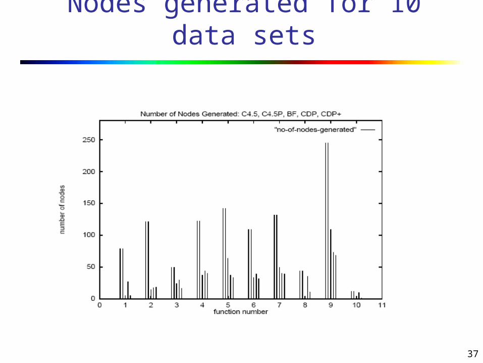
The generation efficiency of the nodes is measured in terms of the total number of nodes generated.
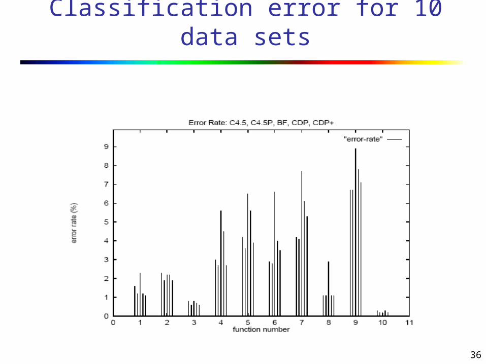
To compare accuracy of the various algorithms, the mean classification error on the test data sets have been computed.
36
Classification error for 10 data sets
37
Nodes generated for 10 data sets

38
Final decision tree size
39
Results/Conclusion
CDP has accuracy comparable to C4.5 while generating considerably fewer nodes.
CDP+ has accuracy comparable to C4.5 while generating considerably fewer nodes.
CDP+ outperformed CDP in error rate and number of nodes generated.
Considering all performance metrics together, CDP+ is the best overall algorithm.
Considering classification accuracy alone, C4.5P is the winner.
40
Conclusion
Different datasets require different algorithms for best results.
Diverse user requirements put different constraints on the final decision tree.
The experiment shows that Interactive Visual Data Mining Framework can help find the most suitable algorithm for a given data set and group of user requirements.
41
Data Mining for Selective Visualization of Large Spatial
Datasets
Proceedings of 14th IEEE International Conference on Tools with Artificial Intelligence
(ICTAI'02), 2002. Washington (November 2002), DC, USA,
Shashi Shekhar, Chang-Tien Lu, Pusheng Zhang, Rulin Liu
Computer Science & Engineering DepartmentUniversity of Minnesota
42
References
http://citeseer.ist.psu.edu/cache/papers/cs/27216/http:zSzzSzwww-users.cs.umn.eduzSzzCz7EctluzSzPaperTalkFilezSzits02.pdf/shekhar02cubeview.pdf
http://www.cs.umn.edu/Research/shashi-group/
http://www.cs.umn.edu/Research/shashi-group/Book/sdb-chap1.pdf
http://www.cs.umn.edu/research/shashi-group/alan_planb.pdf
http://coblitz.codeen.org:3125/citeseer.ist.psu.edu/cache/papers/cs/27637/http:zSzzSzwww-users.cs.umn.eduzSzzCz7EpushengzSzpubzSzkdd2001zSzkdd.pdf/shekhar01detecting.pdf

43
Basic Terminology
Spatial databases Alphanumeric data + geographical cordinates
Spatial mining Mining of spatial databases
Spatial datawarehouse Contains geographical data
Spatial outliers Observations that appear to be inconsistent with
the remainder of that set of data
44
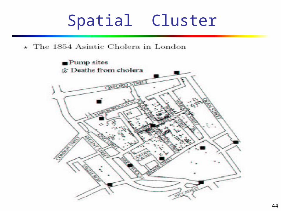
Spatial Cluster

45
Contribution
Propose and implement the CubeView visualization system
General data cube operations Built on the concept of spatial data
warehouse to support data mining and data visualization
Efficient and scalable spatial outlier detection algorithms
46
Challenges in spatial data mining
Classical data mining - numbers and categories. Spatial data – more complex and extended objects such as points, lines and
polygons.
Second, classical data mining works with explicit inputs, whereas spatial predicates and attributes are often implicit.
Third, classical data mining treats each input independently of other inputs.
47
Application Domain
The Traffic Management Center - Minnesota Department of Transportation (MNDOT) has a database to archive sensor network.
Sensor network includes about nine hundred stations each of which contains one to four loop detector
Measurement of Volume and occupancy. Volume is # vehicles passing through station in
5-minute interval Occupancy is percentage of time station is
occupied with vehicles

48
Basic Concepts
Spatial Data Warehouse Spatial Data Mining Spatial Outliers Detection
49
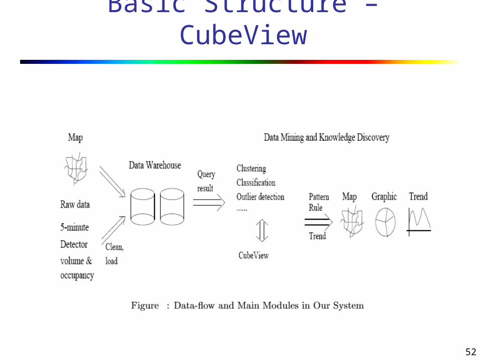
Spatial Data Warehouse
Employs data cube structure Outputs - albums of maps. Traffic data warehouse
Measures - volume and occupancy Dimensions - time and space.

50
Spatial Data Mining
Process of discovering interesting and useful but implicit spatial patterns.
key goal is to partially ‘automate’ knowledge discovery
Search for “nuggets” of information embedded in very large quantities of spatial data.

51
Spatial Outliers Detection
Suspiciously deviating observations Local instability Each Station
Spatial attributes – time, space Non spatial attributes – volume, occupancy
52
Basic Structure – CubeView
53
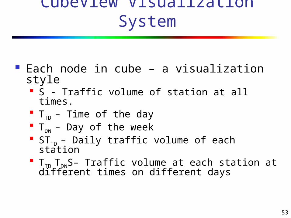
CubeView Visualization System
Each node in cube – a visualization style S - Traffic volume of station at all times. TTD – Time of the day TDW – Day of the week STTD – Daily traffic volume of each station TTD TDWS– Traffic volume at each station at
different times on different days
54
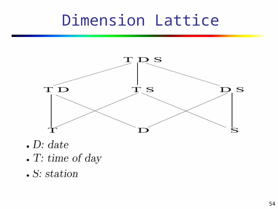
Dimension Lattice

55
CubeView Visualization System
56
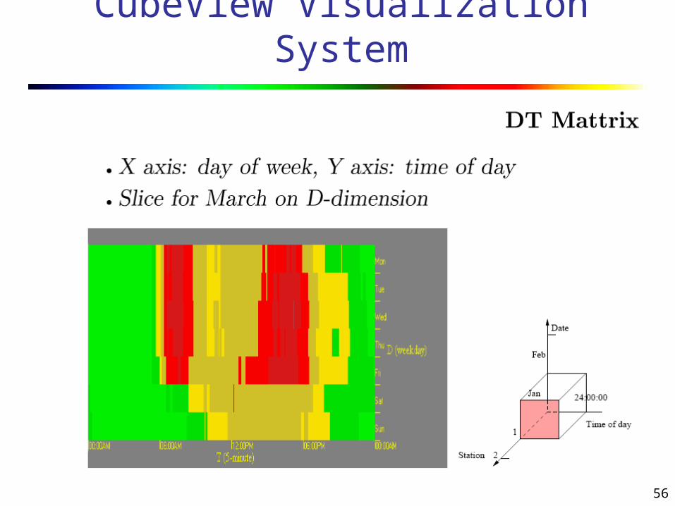
CubeView Visualization System

57
CubeView Visualization System
58
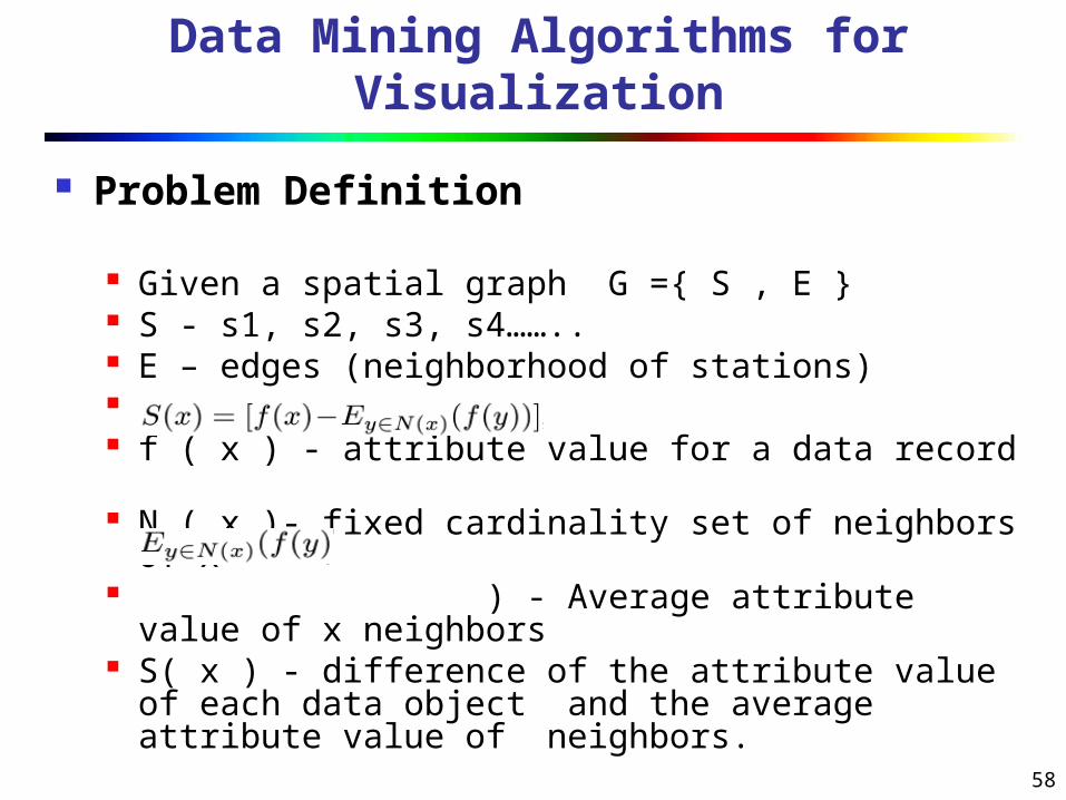
Data Mining Algorithms for Visualization
Problem Definition
Given a spatial graph G ={ S , E } S - s1, s2, s3, s4…….. E – edges (neighborhood of stations) f ( x ) - attribute value for a data record N ( x )- fixed cardinality set of neighbors of x ) - Average attribute value of x
neighbors S( x ) - difference of the attribute value of each
data object and the average attribute value of neighbors.

59
Data Mining Algorithms for Visualization
Problem Definition cont…
S( x ) - difference of the attribute value of each data object and the average attribute value of neighbors.
Test for detecting an outlier
confidence level threshold θ

60
Data Mining Algorithms for Visualization
Few points
First, the neighborhood can be selected based on a fixed cardinality or a fixed graph distance or a fixed Euclidean distance.
Second, the choice of neighborhood aggregate function can be mean, variance, or auto-correlation.
Third, the choice for comparing a location with its neighbors can be either just a number or a vector of attribute values.
Finally, the statistic for the base distribution can be selected as normal distribution.

61
Data Mining Algorithms for Visualization
Algorithms
Test Parameters Computation(TPC) Algorithm
Route Outlier Detection(ROD) Algorithm

62
Data Mining Algorithms for Visualization

63
Data Mining Algorithms for Visualization

64
Data Mining Algorithms for Visualization
65
Software
http://www.cs.umn.edu/research/shashi-group/vis/traffic_volumemap2.htm
http://www.cs.umn.edu/research/shashi-group/vis/DataCube.htm
66
Visualization and Data Mining techniques
Thank you!!!!