1

VM Scaling and Load Balancing via Cost Optimal

MDP Solution

Mark Shifrin, Roy Mitrany, Erez Biton, Omer Gurewitz

Abstract

We address a cost optimization problem faced by a user who runs instances of applications in a remote

cloud configuration constructed of multiple virtual machines (VMs). Each VM runs a single application instance

which can execute tasks specific to that application. Managing the VMs involves a sophisticated trade-off between

cloud-related demands, which are expressed by the provisional costs of leased cloud resources, and exogenous cost

demands expressed by service revenues that are typically bound to service level agreements (SLAs). The internal

costs may include VM deployment/termination cost, and VM lease cost, per time unit. The exogenous costs refer

to rewards accumulated due to the successfully accomplished tasks being run by each application instance. In the

case where the SLA restricts performance to a certain load level at each VM, tasks incoming at VMs that reached

that level are rejected. Rejections cause fines deducted against the rewards. In addition, the performance level is

also quantified, namely, by means of a delay cost, according to the average delay experienced by tasks. Typical

examples for specific applications which fall within this class of problems include handling of scientific worklflows

and network functioning virtualization (NFV). In the latter case the rejection penalties are particularly high.

We model this problem by cost-optimal load balancing to a queuing system with a flexible number of queues,

where a queue (VM) can be deployed, can have a task directed to it and can be terminated. We analyze the

system by Markov decision process (MDP) and numerically solve it to find the optimal policy, which captures

the aforementioned costs and performance constraints. Within this constrained framework, we also investigate the

impact of average VM deployment time. We show that the optimal policy possesses decision thresholds which

depend on several parameters. We validate policies found by MDP, through directing an exogenous computational

tasks flow, which is typical of image processing, to a set-up implemented on AWS. The policy which we propose

here can be adopted by any cloud infrastructure.

I. INTRODUCTION

Cloud computing is a distributed paradigm which enables remote usage of resources (such as servers,

storage, applications and information), by a vast user population distributed over the world. These cloud

arX

iv:1

611.

0695

6v2

[cs

.NI]

4 A

pr 2

019

2

resources are typically allocated in the form of virtual machines (VMs) which are assigned to cloud users

(typically applications) on a rental basis on demand 1. Obviously, to support the enormous number of

applications utilizing the cloud and the large variability of incoming requests, a dynamic resource allocation

mechanism is essential. Such resource allocation mechanisms are essential both by cloud providers who

provide the infrastructure and the consumers, the applications. The objectives and constraints of either

are not necessarily aligned and sometimes are even opposed. Specifically, on the one hand the cloud

provider needs to place the VMs on physical machines taking into account various constraints such as

determining which physical machine best suits each VM’s requirements, spreading VMs over multiple

physical machines for fault tolerance. Moreover, it needs to overcome failures, and accommodate bursty

VM requests trying to admit all incoming requests, to ensure load balancing while cutting expenses,

increasing revenue, etc. On the other hand, the user utilizing the cloud (an application) is charged based

on the resources (VMs) it retains. Its incentive is to lower costs, hence to utilize as few VM resources

as possible. On the other hand, the number of requests from the applications consumers, handled by a

VM hosting the application can affect performance (e.g., many requests, higher latency). Accordingly, the

application aspires to deploy a dynamic resource allocation mechanism which adopts the number of leased

VMs to the current demands. Due to its high importance and its impact on bringing cloud computing to

more domains in our daily life, both aspects of resource allocation have drawn a lot of attention over

the last few years both by the industry and by the academy. Notably, for most objectives the resource

allocation problem is an NP-hard optimization problem (see, e.g., [4], [16] for the problem hardness

discussion). Throughout this paper we concentrate on the applications mechanism. We assume that the

cloud providers are abundant with resources which they lease on request, and charge the application based

on various pre-agreed parameters, such as the cost per VM, installing or removing VMs, etc.

As mentioned, the trade-off between performance and number of VMs an application acquires, ne-

cessitates a dynamic resource allocation mechanism which increases or decreases the resources, in the

form of VMs, to fulfill the elastic demands of the application. Such adaptive resource allocations are

typically attained via two mechanisms, load balancing and scaling. Load balancing is responsible for

distributing the application traffic-load or application requests between the leased VMs, such that no VM

is overloaded while others are less congested. Scaling refers to the procedure of adding (scale-out) or

1Even though our method applies both for public and private clouds, for clarity we will mostly refer to public cloud

3

releasing (scale-in) VMs according to the demand 2. Clearly, the scaling mechanism which dynamically

adds or removes resources (VMs) needs to ensure that the applications clients will be satisfied and if

there exists a Service Level Agreement (SLA) between the application and its consumers, it is kept.

Accordingly, the dynamic resource allocation mechanism should balance financial considerations (e.g.,

adding or maintaining unnecessary VMs) and user satisfaction (e.g., performance).

Common application-resource-allocation mechanisms utilize an on demand approach, aiming at maxi-

mizing resource utilization by means of avoiding both overload and underload of VMs while maximizing

users performance, typically consent with users SLA. However, it is clear that without pre-planning and,

specifically, without trying to predict future demands, the resources maintained by an application can be

satisfactory on the short term, yet badly utilized on the long run. Furthermore, due to its commercial

nature, there are other perspectives, besides the complying with the SLAs, that should be considered. For

example, due to the cost-effect reasoning, a user can prevent adding a VM (scaling out), thus compromising

performance, or even risk a rejected task allocation request, or, on the contrary, bear the cost of multiple

active yet underutilized VMs, in order to avoid future performance degradation and/or a rejection. In

addition, a user can decide to migrate tasks from one VM to others in order to terminate a VM and

save the expense or not to divert traffic to a VM in order to release it in the near future. Typically, the

cloud providers implement application programming interfaces (APIs) for applications to set up several

predefined parameters (thresholds) for execution scale out/in. However, a cloud user, who deploys an

application(s) for clients, and reduces costs by controlling its own scaling and load balancing mechanisms,

needs to take all these considerations into account, dynamically and automatically, transparently to the

clients using the application, and without altering the application with respect to each action taken.

To this end, the set of costs incurred by the application can be conceptually divided into two types: the

provisional costs (PC) and service revenues (SR). PC refer to the payments incurred by the cloud provider,

i.e., the costs that the cloud provider charges the cloud hosts (the applications) for utilizing its resources.

These costs are typically per resource utilization (e.g., the number of VMs the application utilizes per unit

time, the cost for acquiring or releasing a VM, etc.). The SR refer to the costs which are exogenous to the

cloud and stem from the SLA (with exogenous clients) and the performance level measured by the cloud

user, i.e., the enterprise through its cloud exploitation. Specifically, the PC are accumulated continuously

2Scaling also refers to the procedure of adding or removing resources such as computing power, memory, storage, or network capabilities,to an existing machine (termed Scale-up and Scale-down, respectively). This procedure is not common hence will not be addressed throughoutthis paper.

4

according to the retained resources (VMs) which are controlled dynamically via the application scaling

mechanism. Namely, an enterprise which runs the application decides on scale out/in operations which

increase/decrease (i.e., deploy/terminate) the number of VMs, respectively. Obviously, utilizing scale up

and down mechanisms which can upgrade (add resources to) or downgrade (remove resources from)

existing VMs, can also effect the PC, however these procedures which are not broadly supported (e.g.,

they are not supported by Amazon Web Services (AWS) which we exploit throughout this paper) and are

not addressed in this paper. On the other hand, scale up and down mechanisms do affect SR by various

factors. The foremost factor is the performance which is directly affected by load on each VM, which

is affected by both the scaling and load balancing mechanisms. Note that the effect on performance is

not necessarily a simple function of the number of employed VMs or the number of users utilizing the

application. For example, the expected delay experienced by a video streamer request, definitely relies on

the load of the VM which addresses this request, however it relies on several other factors (such as the

negative impact of other requests being concurrently served on the same VM ) and is not necessarily a

linear function of the load. In our mathematical formulation, we address this generality.

Throughout this paper, we will assume that the PC are typically set according to a price-list which is

agreed upon on advance (note that in private clouds it is possible to quantify the costs of utilizing resources

as well). As for the SR, it is expressed via rewards or fines, associated with successfully processed or

rejected tasks, respectively. We assume that these costs are negotiable between the application and its

users, yet this is determined a-priori (e.g., via SLA). In order to materialize the service quality associated

with the performance (e.g., delay), we translate it to performance costs which stand for additional fines

inflicted on the enterprise, thus encouraging faster processing. Typically, the calculation of these costs is

implemented by means of pre-negotiated delay cost factors (DCF) which appropriately scale the delay

function. The DCF value versus the experienced delay provide an additional complexity to the problem.

We term by cost parameters (CP) the fixed set of all costs VM deployment/termination cost, DCF, reward,

rejection fine and VM holding cost.

In this paper, we explore and formulate the enterprises objective of optimizing its revenues under the set

of costs. Specifically, we devise a decision maker (DM) which implements optimal scaling, load balancing

and admittance control, based on the predefined CP and the current known system state.

Scaling and load balancing in the cloud has drawn a lot of attention over the last few years both by

the academy and by the industry; many studies have addressed the problem of dynamic scaling in the

5

cloud. The review on cloud auto-scaling [18] would categorize our work within a class of reinforcement

learning (RL-based) scaling techniques, as in, e.g., [28] which utilizes Q-learning for resource allocation

in data center. Yet, works mentioned wherein do not account for load balancing and do not capture the

cost trade-offs we address. Another class of works ( [7]) concentrate on architectural novelties, while the

scaling is governed by heuristically set thresholds. The recent survey in [31] on load balancing reasons

the NP-hardness of the general LB problem in cloud and categorizes the existing algorithms into heuristic

and meta-heuristic. However, we argue that for the carefully defined assumptions, an optimal solution

can be presented, without sacrificing the major part of the generality. Hence, this paper is the first to

give a mathematical formulation from the perspective of the enterprise’s long-run cost optimization, while

capturing the trade-off structure in this degree of generality. The solution we provide directly leads to

the practical methodology, to be implemented within existing or yet-to-come scaling and load balancing

architectures.

To this end, we model the problem by a queuing system with a dynamic yet limited number of queues.

The controllable queuing system represents the dynamic VM deployment and tasks balancing problem

which we treat by introducing a stochastic control model based on Markov decision process (MDP)

formulation. The solution to the MDP provides the optimal policy.

While the set of costs described above implies no trivial policy could exist, some of the parameters

have contradicting impacts which may dictate certain properties of the policy. For example, in the case

where the delay cost function sharply increases with the load, the DM will attempt to deploy as many

VMs as possible. On the other hand, in the case where keep-alive cost is comparatively high, the DM

may prioritize minimization of the active VMs number. A distinctive impact has a VM deployment time,

which we separately explore.

Once applied, the policy potentially reveals the optimal average number of active VMs and the cor-

responding optimal average number of tasks in the queue associated with the VMs. This allows the

enterprise to assess the demands and to plan ahead. Moreover, the solution to the MDP is expressed by

value function which indicates what are the costs and revenues the enterprise will receive in the long run,

for a given scenario along with its set of parameters.

To summarize, the contribution of this paper is as follows:

• We formulate load balancing of task arrivals and VM scaling problem by stochastic model solvable

by MDP.

6

• The MDP is numerically solved providing the optimal policy which captures the various costs

constraint.

• A detailed research of the value function structure is performed and the insights of the structure of

the optimal policies are brought.

• We separately investigate the impact of the VM deployment time.

• We built a simulation set-up on the basis of AWS platform and apply the policy retrieved from MDP

solution.

Note that this set of constrains we considered was more elaborate than AWS setting allows. Hence, while

we used AWS for the exemplifying purposes, the method we present in this paper is generic, and will

fit any cloud based platform. The only needed input for the MDP consists of system parameters (e.g.

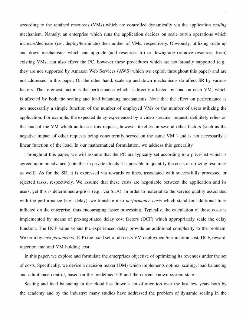
average VM deployment time, average task execution time). The implementation methodology, which

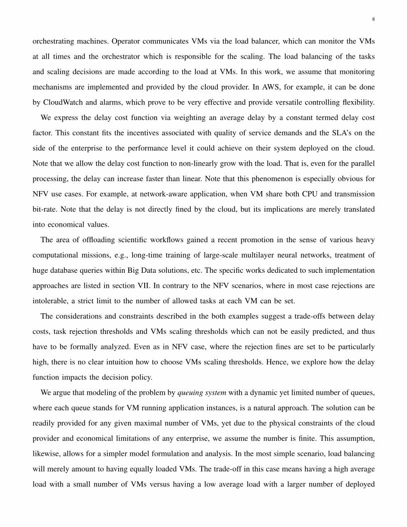
is suggested to be harnessed by enterprises, may be expressed by a closed loop, as it is schematically

depicted in Figure 1.

Fig. 1. Policy calculation closed loop. The scaling time statistics

are firstly measured for an arbitrary policy and then used for the

optimal policy calculation. At least one additional measurement

is needed to adjust to the impact of the MDP driven policy.

The rest of the paper is organized as follows.

The next section provides general background on

VM control in cloud computing, by exemplifica-

tion via NFV and scientific workload scenarios.

This part might be familiar to the experts in cloud

computing. We provide system description in sec-

tion III. Section IV provides the MDP formulation.

The study of the optimal policy and of the impact

of different parameters is discussed in Section V.

Section VI provides the review of our AWS-based implementation and demonstrates the results of applying

the optimal policy on AWS. Section VII gives the related work and concludes this paper.

II. VM CLOUD-BASED CONTROL BACKGROUND

We provide preliminaries and bring the related examples which demonstrate the problem of VM control

in practice. We rely on two scenarios. The first one is driven from NFV paradigm while the second one

is from offloading massive scientific computation workloads. Both examples are characterized by the

tension raised by an enterprise’s aim to maximize the revenues accumulated in the process of successful

task execution, on the one hand, and keeping the cloud expenditures as low as possible, on the other hand.

7

The breakthrough of the NFV concept gave rise to novel demands triggered by the goal to cost-effectively

run persistent networking functionalities. Fulfilling the cost optimality demands, in NFV context, implies

binding VM deployment with solutions to variety of networking aspects. Fo the clarity, we name three

possible interacting sides as follows: 1) The users, who supply the demands, 2) The operator which is

responsible for all control decisions and 3) The cloud provider which supplies the VMs. Once a VM

is deployed, it is uniquely associated with a specific task type, which is related to a specific virtual

networking function (VNF). Note that two possible configurations of deployment are possible: A) where

all VMs are deployed over the remote cloud. In this case all HW-related costs are paid by operator to the

cloud provider and B) The cloud is private and is actually owned by the operator. The costs are associated

with the operator’s activities for handling the owned VMs.

A deployed VM, which is normally started with an image containing the desired VNF, is disposed to

handle a flow of latency sensitive tasks (according to the SLA) which are typically directed to it by a

separately (on-premises or externally) implemented orchestrator which combines in itself a decision maker

(DM) which is responsible for scaling. In addition, there is an virtualized entity which is responsible for the

load balancing. (It may be deployed separately from an orchestrator.) We assume that the functionality

type of VNF of interest is known and fixed, and that there is a constant influx of tasks to be served

by the corresponding VMs deployment, where all such VMs have instances of the corresponding VNF

implemented on them.

The procedure of deployment takes time which depends on various factors which include the type of

VM, availability, booting time, and deployment of the image which includes the application. We account

for a one-time deployment and termination cost applied for each VM. In the case these costs are not

applied at a specific cloud provider, they are just assumed to be zero in the model formulation. Once

deployed, the operator pays per time of having the deployed VMs, regardless of the load. This cost is

charged per unit of VM’s leased time. In AWS, for example, the payment is normally applied per hour

of a usage. Alternatively, in a private cloud owned by the operator, the payments are related to costs

of not leasing those VMs for other revenue making applications. The tasks are directed to VMs upon a

connection establishment via the load balancer (LB). The LB might be separately defined and deployed

by an operator who sets its configuration, yet physical details might be left transparent3. For simplicity,

our model does not account for the costs associated with the deployment of the load balancing and

3The alternative, where the operator would not use cloud provider controlling tools is also possible. In this case she will implement herown load balancing and orchestrating SW and will use it for addressing VMs.

8

orchestrating machines. Operator communicates VMs via the load balancer, which can monitor the VMs

at all times and the orchestrator which is responsible for the scaling. The load balancing of the tasks

and scaling decisions are made according to the load at VMs. In this work, we assume that monitoring

mechanisms are implemented and provided by the cloud provider. In AWS, for example, it can be done

by CloudWatch and alarms, which prove to be very effective and provide versatile controlling flexibility.

We express the delay cost function via weighting an average delay by a constant termed delay cost

factor. This constant fits the incentives associated with quality of service demands and the SLA’s on the

side of the enterprise to the performance level it could achieve on their system deployed on the cloud.

Note that we allow the delay cost function to non-linearly grow with the load. That is, even for the parallel

processing, the delay can increase faster than linear. Note that this phenomenon is especially obvious for

NFV use cases. For example, at network-aware application, when VM share both CPU and transmission

bit-rate. Note that the delay is not directly fined by the cloud, but its implications are merely translated

into economical values.

The area of offloading scientific workflows gained a recent promotion in the sense of various heavy

computational missions, e.g., long-time training of large-scale multilayer neural networks, treatment of

huge database queries within Big Data solutions, etc. The specific works dedicated to such implementation

approaches are listed in section VII. In contrary to the NFV scenarios, where in most case rejections are

intolerable, a strict limit to the number of allowed tasks at each VM can be set.

The considerations and constraints described in the both examples suggest a trade-offs between delay

costs, task rejection thresholds and VMs scaling thresholds which can not be easily predicted, and thus

have to be formally analyzed. Even as in NFV case, where the rejection fines are set to be particularly

high, there is no clear intuition how to choose VMs scaling thresholds. Hence, we explore how the delay

function impacts the decision policy.

We argue that modeling of the problem by queuing system with a dynamic yet limited number of queues,

where each queue stands for VM running application instances, is a natural approach. The solution can be

readily provided for any given maximal number of VMs, yet due to the physical constraints of the cloud

provider and economical limitations of any enterprise, we assume the number is finite. This assumption,

likewise, allows for a simpler model formulation and analysis. In the most simple scenario, load balancing

will merely amount to having equally loaded VMs. The trade-off in this case means having a high average

load with a small number of VMs versus having a low average load with a larger number of deployed

9

VMs. This is the scenario we test on AWS setup, as is explained in section VI. However, having in

mind deployment time and cost, this trade-off still represents a significant challenge as the optimal policy

derivation is not straightforward.

We additionally assume that the VM placement problem and authentication issues are independently

solved prior to the scheduling, and that the solutions are static or have no effect on scheduling-related

parameters (e.g. VM deployment time.) Henceforth we focus on the cost-optimal VM scaling and the

load balancing challenges which are relevant for a given specific type of tasks. In order to circumvent

privacy-related issues, we also assume that all tasks are coming from the same user identity. Extending

to several users or/and to several task types is straightforward and merely converges to solving several

independent problems, where only minor adjustments to the setting are needed.

Note that NFV and offloading workflows are only a portion of the possible scenarios that can be

associated with the described system. We believe that NFV is a best exemplifying candidate both because

of its global nature and of the fact that it is clearly associated with a persistent long-term task flows.

Hence it constitutes an obvious yet open and important problem of long-run cost optimization. Any other

entity with persistent flows of tasks can be considered, provided it introduces the appropriate translations

of task completion successes and failures to the rewards and fines.

For the sake of exemplification, we will use NFV terminology whenever further detailed exemplification

is needed.

III. FORMAL SYSTEM DEFINITION

We assume that the available cloud resources (e.g., NFV infrastructure) can host a finite yet flexible

number of VMs. We further assume, that a load balancer (LB) is deployed and can handle all traffic

demands irrespective of the number of VMs, see Figure 2 for the schematic presentation.

Our theoretical model is based on a Markovian assumption. That is, the service demand is modeled by

a Poisson process of arriving tasks with average rate λ. Upon each task arrival event, (service request), the

decision making (orchestrator) decides whether to instantiate a new queue (VM) to handle the demand, as

long as the maximal number of active queues (VMs) is not reached. In addition, it directs the task towards

a load balancer, which balances tasks across active queues. Once service is ended (i.e., task departure)

and a VM is left idle (the queue is left empty), the orchestrator may keep the VM or destroy it. In what

follows, we will use naming Decision Maker (DM) in order to refer to the operator and queue in order

to refer to a VM.

10

The maximal number of running task on a single VM is limited by the borderline number, above it the

performance degrades below the minimal quality of service and, hence, should never be exceeded.

The DM aims to find a policy which maximizes the total income in the long run. We assume expo-

nentially distributed service time and a time it takes from the moment of VM deployment decision till

the moment it is fully deployed. While the arrival part of the Poisson assumption is rather natural, the

same assumption about the service and deployment part mean that we impose an approximation of the

service times and on VM deployment times. However, the drawback of this approximation proved to be

non-significant, as show our results in Section VI. Moreover, to account for general (but known) service

times, it is merely needed to extend our MDP model to a Semi-Markov Decision Process (SMDP) model,

an effort that is purely technical. As the objective of this work is to present a general methodical paradigm,

we leave the extension to SMDP out of the scope of this paper. Accordingly, incoming tasks are scheduled

to one of the active queues or rejected from service, according to the load balancing policy. Each VM can

handle services in a parallel manner. Namely, the total processing rate is equally shared between all tasks

currently running in the queue. Hence, tasks never wait for a full completion of previously arrived tasks

but are rather processed in parallel. The VM’s limited resources allow processing of a limited number of

services, denoted by B. The parameter B is calculated based on the service SLAs. We omit these detailed

calculations and assume B is given. For simplicity, we assume all VMs are identical, hence characterized

by equal B. We assume that the exponential service times have maximal average rate µ. We assume that

task processing initiation at each VM has no time overhead. However, VM deployment time is significant.

For analytical simplicity we also assume it is exponentially distributed with average rate ζ . Each VM is

modeled by a queue with a buffer size B, having up to B servers with a total processing rate equal to

µ. Since the minimum of exponentially distributed rates is equal to their sum, the total processing rate is

always equal to µ. While this model reflects the ability of VMs to provide concurrent resource sharing, it

can be easily modified for the FIFO service, with only minor changes. Note that for the correspondence

with the mathematical model, which will follow, we use the terms VM and queue interchangeably.

The Service revenues (SR) are primarily composed of rewards for admitted tasks and fines for rejected

tasks. We assume that an admitted task gives a fixed reward, while a rejected task incurs a fine, denoted by

{r, f}, respectively. Intuitively, the number of queues may infinitely grow for some sets of parameters, as

long as the total cost is minimized. For example, in the case where λ� µ, and rejected tasks incur high

fines, it always profitable to have as many VMs deployed as needed in order to avoid tasks rejections.

11

On the other hand, the number of available queues is expected to be bounded by both general system

limitations and economic considerations. We will naturally assume henceforth that the number of active

queues is limited. In case that there is no active VM, i.e., immediately after the VNF on-boarding and

before its VM deployment or in case that all active VMs are overloaded and cannot accommodate new tasks

an incoming task would be rejected. However, for the hypothetical configuration where the deployment

time is instantaneous, rejection could be avoided by an immediate VM deployment. This configuration

merely has theoretical value and is unpractical. Hence we will assume for our validation setup that the

deployment time is not negligible at all times. Furthermore our equations account for the deployment

times.

Set of the queues

We define next vector of queues, which describes both the state of all queues and the number of tasks

in each one of them. Hence, such a vector uniquely reflects the system state. We will need the following

definition for this purpose. Denote the set q = {−2,−1, 0, · · · , B}. The vector of all queues at time t is

denoted by q(t). The maximal number of VMs is given by the size of this vector, namely |q| = n, for

some system-related n which was precalculated and fixed. The state-space (st.-sp.) defines all possible

states the VMs (queues) could possibly have. Denote it by the following

Q = qn ,q(t) ∈ Q

The components of q(t) correspond to the number of tasks in queues and are denoted by qi(t), where i

is the general indexing of the queues. To this end, qi ∈ q. The state ”−2” means the queue is inactive

and state ”−1” means the queue is being currently deployed. Note that this is different from state 0

which means the queue is active and deployed, but empty. (We will omit the time notation in cases

where the current time is of no importance to the analysis.) While for simplicity we assumed µi = µ, the

extension to the system with different processing rates is straightforward, at expense of the appropriate

st.-sp augmentation. The number of all states is denoted by |Q|. We will use the definition of the state

space Q in the next section for the formal MDP formulation.

Cost structure

We now formally define the cost parameters which can be logically divided to the provisional costs

(PC) and the service revenues (SR). We define first the structure of the delay cost. Denote by h the delay

12

cost per unit of processing time, associated with a number of hosted tasks. That is, h serves as a delay

cost factor (DCF) responsible for the part of the SR which associate the SLA with the performance level.

At ith queue, at time t, cost equal to hi(t) per unit of time is inflicted. The delay cost model is represented

by function which increases with the number of hosted tasks at VM. This structure reflects a load increase

(and, consequently, the overall queuing time) with the number of residing tasks at a VM. In particular we

express this load impact by using an increasing function η as follows,

hi(t) = qi(t)η(qi(t))h, (1)

Where η ≥ 1 for all possible qi values and is positive increasing with qi. Namely, more busy VMs perform

with higher delay. Hence, this cost structure penalizes for having busy VMs. Therefore, this formulation

allows to capture parallel processing, such that the delay cost of all running tasks is appropriately weighted

by their quantity at a VM. Note that if we assume η(i) = 1 for all i, the cost will degenerate to the simple

linear model. The cumulative delay cost till time mark t is merely given by

Hi(t) =

∫ t

0

qi(t)η(qi(t))h dt

The DCF, together with earlier defined rewards and fines {r, f} accomplish the definition of SR. As

for cost parameters related to PC, the deployment cost β is applied each time a queue is activated. The

termination cost ψ is applied each time a queue is terminated. Observe that the total delay cost is the

lowest when tasks are equally dispersed over queues. Once a VM is empty no delay cost is applied,

however the keep-alive cost for having a deployed VM is always charged, even if the VM was idle.

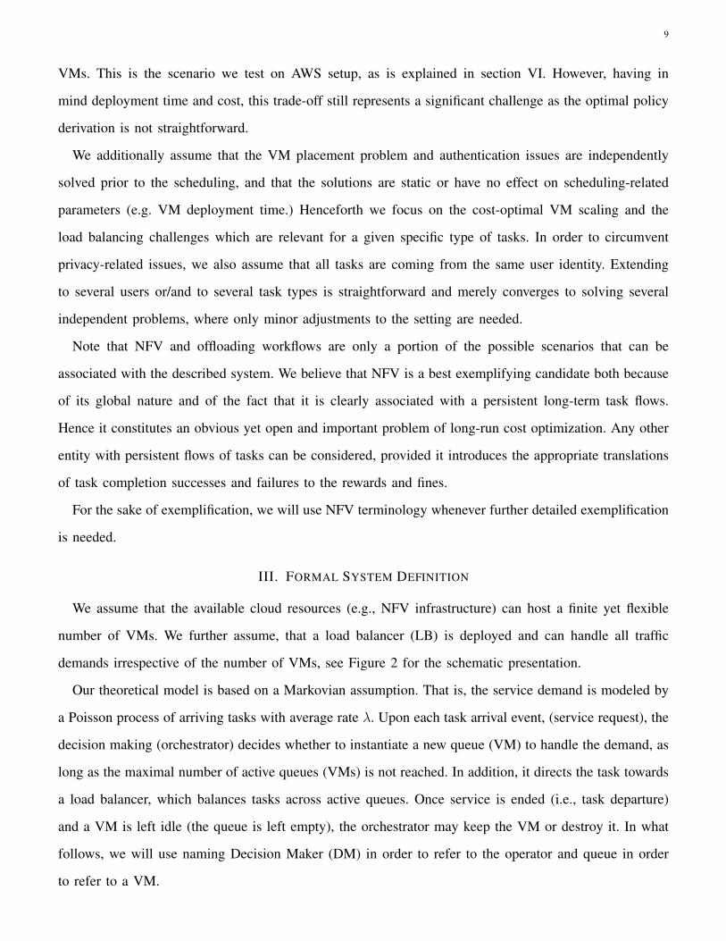
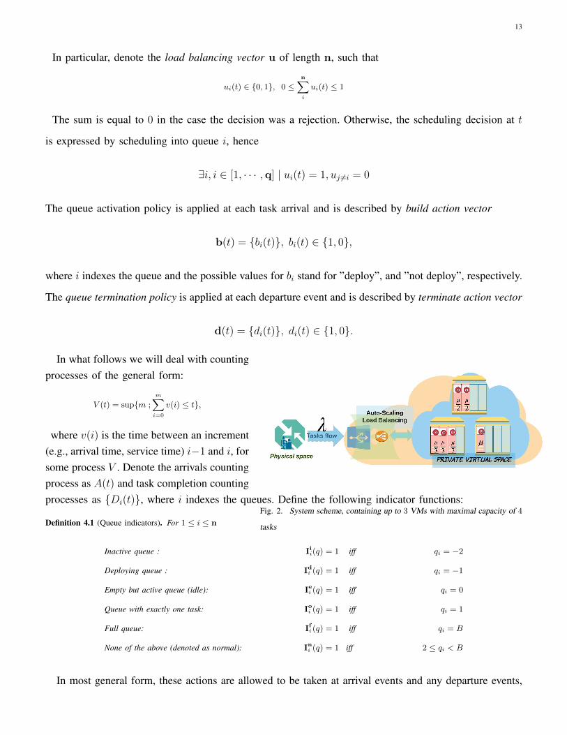
Denote this cost by κ per a time unit. This cost is also a part of PC. Figure 2 depicts a physical enterprise

which constantly offloads tasks with average rate λ to his virtual private space which contains up to 3

VMs, where minimal tolerable service rate is given by µ4.

We are now disposed to formulate the MDP.

IV. MDP FORMULATION

We define the action space first, denote it by A. Denote action a ∈ A at time t as

a = {u,b,d}

13

In particular, denote the load balancing vector u of length n, such that

ui(t) ∈ {0, 1}, 0 ≤n∑i

ui(t) ≤ 1

The sum is equal to 0 in the case the decision was a rejection. Otherwise, the scheduling decision at t

is expressed by scheduling into queue i, hence

∃i, i ∈ [1, · · · ,q] | ui(t) = 1, uj 6=i = 0

The queue activation policy is applied at each task arrival and is described by build action vector

b(t) = {bi(t)}, bi(t) ∈ {1, 0},

where i indexes the queue and the possible values for bi stand for ”deploy”, and ”not deploy”, respectively.

The queue termination policy is applied at each departure event and is described by terminate action vector

d(t) = {di(t)}, di(t) ∈ {1, 0}.

Fig. 2. System scheme, containing up to 3 VMs with maximal capacity of 4

tasks

In what follows we will deal with countingprocesses of the general form:

V (t) = sup{m ;

m∑i=0

v(i) ≤ t},

where v(i) is the time between an increment(e.g., arrival time, service time) i−1 and i, forsome process V . Denote the arrivals countingprocess as A(t) and task completion countingprocesses as {Di(t)}, where i indexes the queues. Define the following indicator functions:

Definition 4.1 (Queue indicators). For 1 ≤ i ≤ n

Inactive queue : Iii(q) = 1 iff qi = −2

Deploying queue : Idi (q) = 1 iff qi = −1

Empty but active queue (idle): Iei (q) = 1 iff qi = 0

Queue with exactly one task: Ioi (q) = 1 iff qi = 1

Full queue: Ifi (q) = 1 iff qi = B

None of the above (denoted as normal): Ini (q) = 1 iff 2 ≤ qi < B

In most general form, these actions are allowed to be taken at arrival events and any departure events,

14

that is, once the counting processes A and Di increase.Define the infinite horizon discounted cost functional, discounted with discount factor γ, for policy π

as follows:

Jπ =

∫ ∞0

e−γt·[−(b(t) · β + d(t) · ψ

)(dA(t) +

n∑i

dDi(t))

(2)

−n∑i

(hi(t) + κ ∗ (1− Iii)

)dt (3)

+ (u(t) · r − f ∗ (1−n∑i

ui(t))dA(t)], (4)

where hi(t) is substituted from Equation (1). The cost can be divided into the components as follows.

The first part of the display above, i.e. (2), stands for the queue deployment cost, denote it as Jπb , and

termination cost, denote it as Jπd . The second part, i.e. (3), stands for queue holding cost, denote it as

Jπh , and delay cost, denote it as Jπκ . The third part, i.e. (4), stands for the cost associated with scheduling

rewards, denote it as Jπr , and the cost associated with rejection fines, denote it as Jπf . That is, the cost is

otherwise written by using the aforementioned components as follows,

Jπ = −Jπb − Jπd − Jπh − Jπκ + Jπr − Jπf .

The value function associated with initial state q is given by

Vq = maxπ

Jπ(q).

We now write the Bellman equation for a simplified and more realistic scenario assuming that buildoperations can be only done at arrivals, while destroy operations can be only done at departures. Denoteby ei vector of length n with value 1 at ith coordinate and zeros in all other coordinates. The Bellmanequation reads

Vq =[ q∑

i

Ini µiVq−ei +

q∑i

IfiµiVq−ei +

q∑i

Ioi µi max{Vq−ei , Vq−2ei − ψ}+

q∑i

Idi ζiVq+ei

+ λmax{

maxb={0,1}

[max

i,Ifi=0,Idi =0{Vq+ei − bβΠjI

ij + r}

], maxb={0,1}

[Vq − f − bβΠjI

ij

]}+ C(q)

]δq, (5)

where the cost function C(q) and normalization factor δ are calculated by

C(q) =

q∑i

hi + κ ∗ (1− Iii)(1− Idi ), and δq =

q∑i

(1− Iii)(1− Iei )(1− Idi )µi +∑i

Idi ζi + λ+ γ (6)

Note that in the case where all queues are full, the outcome of the inner maximization is empty. Inthis case, the second term in outer maximization is selected. The maximization over deployment decisionwhich is denoted by b is made both in rejection and task scheduling cases. Hence, the decision to reject a

15

task, but to start deployment of a previously idle queue is allowed. See that the product ΠjIij is equal to 1

only in the case at least one queue is non-idle. Otherwise, it is equal to 0 and no actual VM deploymenthappens. In the ideal case of instantaneous VM deployment, that is, when ζi = 0, ∀i, we substituteIdi = 0. The state of being deployed then does not effectively exists, hence write

Vq =[∑

i

Ini µiVq−ei +∑i

IfiµiVq−ei +∑i

Ioi µi max{Vq−ei , Vq−2ei − ψ}+ (7)

λmax{

maxi,Ifi=0

{Vq+ei+Iiiei− βIii + r}, Vq − f

}+ C(q)

]δq,

Observe that the action space is effectively restricted, such that only one queue at each time is allowed tobe deployed, at arrival opportunities. The corresponding newly arrived task will be scheduled at the newlydeployed queue. While it restricts in some sense the action space, this setting is practically reasonable.The derivation of equation (7) can be found in Appendix A. The importance of simplistic version ofthe system described by equation (7) is mostly explorational and it is analyzed in Section V. In V-Bthe impact of the parameter ζ is analyzed. The complete and more realistic system version describedby equation (5) is additionally validated by AWS-based implementation in section VI. Bellman equation,such as (7), belongs to the well known class of equations which are solved by the value function V whichconstitutes a fixed point of an operator which corresponds to the equation. In another words, one definesoperator T acting over V in (7) as follows

T Vq =[∑

i

Ini µiVq−ei +∑i

IfiµiVq−ei +∑i

Ioi µi max{Vq−ei , Vq−2ei − ψ}+

λmax{

maxi,Ifi=0

{Vq+ei+Iiiei− β ∗ Iii + r}, Vq − f

}+ C(q)

]δq, (8)

Since V is a fixed point the display above writes V = T V . The detailed theory behind (8) can be found

in, e.g., [5] and is not elaborated in this paper. We merely present the value iteration algorithm which is

numerically applied in order to calculate V . Denote by Ta application of the operator associated with some

action a ∈ A, that is, each Ta refers to correspondent triplet of actions, namely, to a = {u,b,d}. Then,

the value iteration algorithm is merely given in Algorithm 1. Observe that line 7 amounts to applying T .

That is, maxa Ta = T .Note that the size of of the state space exponentially grows with the maximal number of VMs. For

example, for maximum of 5 VMs, each one is allowed to accommodate up to 5 tasks, we have 5 queueswith 8 possible states each. Hence, in this case,

q = {−2,−1, 0, · · · , 5}, |Q| = 85 = 32768 states. (9)

Therefore, algorithm 1, although is written for simplicity in a scalar form, was carefully treated vector-

wise. See also the implementation comments in the following sections.

16

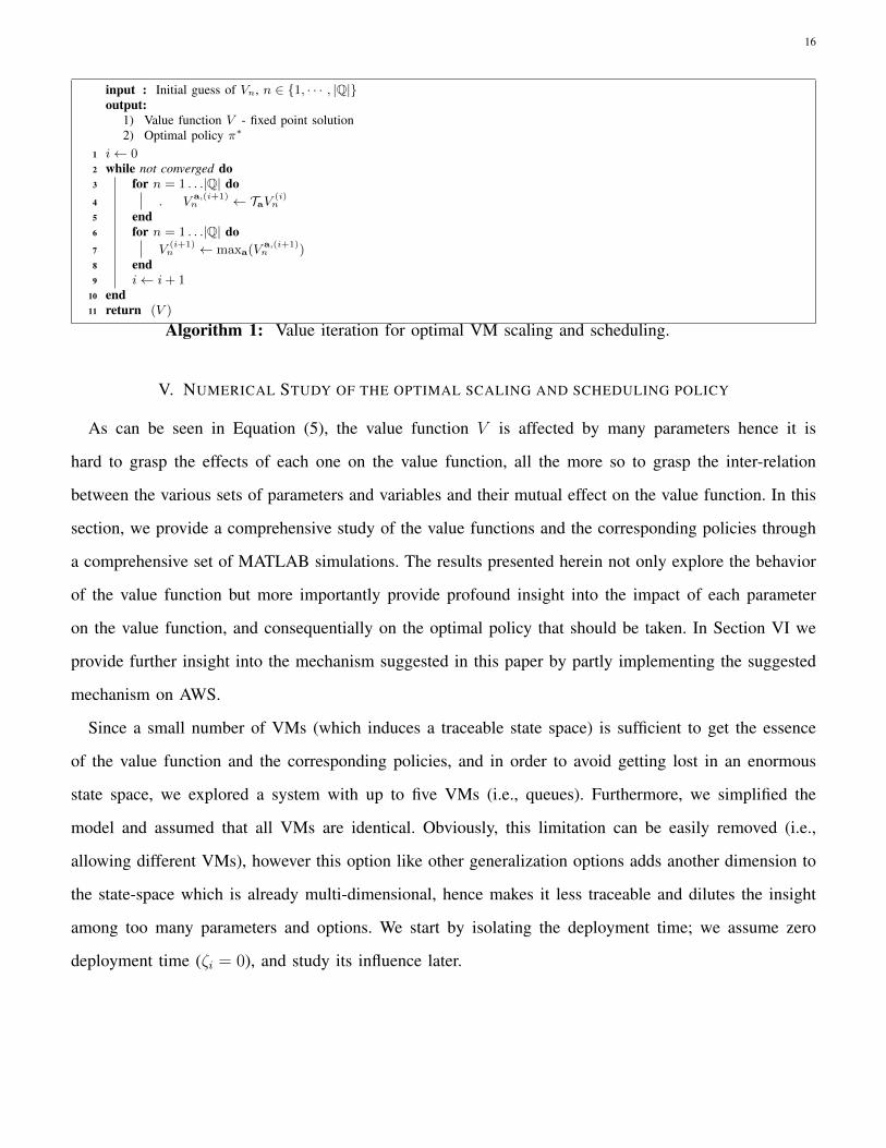
input : Initial guess of Vn, n ∈ {1, · · · , |Q|}output:

1) Value function V - fixed point solution2) Optimal policy π∗

1 i← 02 while not converged do3 for n = 1 . . .|Q| do4 . V

a,(i+1)n ← TaV (i)

n

5 end6 for n = 1 . . .|Q| do7 V

(i+1)n ← maxa(V

a,(i+1)n )

8 end9 i← i+ 1

10 end11 return (V )

Algorithm 1: Value iteration for optimal VM scaling and scheduling.

V. NUMERICAL STUDY OF THE OPTIMAL SCALING AND SCHEDULING POLICY

As can be seen in Equation (5), the value function V is affected by many parameters hence it is

hard to grasp the effects of each one on the value function, all the more so to grasp the inter-relation

between the various sets of parameters and variables and their mutual effect on the value function. In this

section, we provide a comprehensive study of the value functions and the corresponding policies through

a comprehensive set of MATLAB simulations. The results presented herein not only explore the behavior

of the value function but more importantly provide profound insight into the impact of each parameter

on the value function, and consequentially on the optimal policy that should be taken. In Section VI we

provide further insight into the mechanism suggested in this paper by partly implementing the suggested

mechanism on AWS.

Since a small number of VMs (which induces a traceable state space) is sufficient to get the essence

of the value function and the corresponding policies, and in order to avoid getting lost in an enormous

state space, we explored a system with up to five VMs (i.e., queues). Furthermore, we simplified the

model and assumed that all VMs are identical. Obviously, this limitation can be easily removed (i.e.,

allowing different VMs), however this option like other generalization options adds another dimension to

the state-space which is already multi-dimensional, hence makes it less traceable and dilutes the insight

among too many parameters and options. We start by isolating the deployment time; we assume zero

deployment time (ζi = 0), and study its influence later.

17

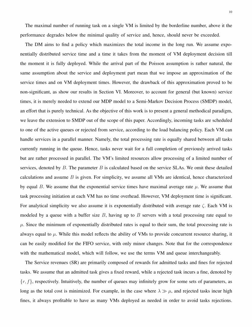
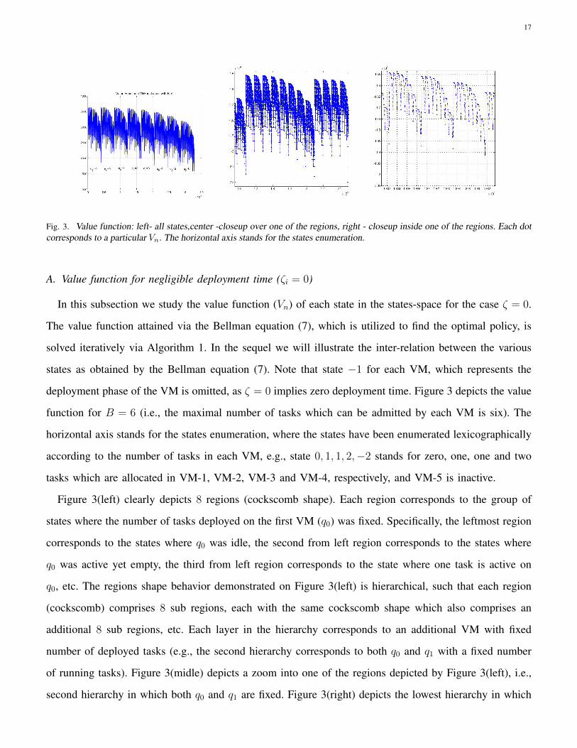
Fig. 3. Value function: left- all states,center -closeup over one of the regions, right - closeup inside one of the regions. Each dotcorresponds to a particular Vn. The horizontal axis stands for the states enumeration.

A. Value function for negligible deployment time (ζi = 0)

In this subsection we study the value function (Vn) of each state in the states-space for the case ζ = 0.

The value function attained via the Bellman equation (7), which is utilized to find the optimal policy, is

solved iteratively via Algorithm 1. In the sequel we will illustrate the inter-relation between the various

states as obtained by the Bellman equation (7). Note that state −1 for each VM, which represents the

deployment phase of the VM is omitted, as ζ = 0 implies zero deployment time. Figure 3 depicts the value

function for B = 6 (i.e., the maximal number of tasks which can be admitted by each VM is six). The

horizontal axis stands for the states enumeration, where the states have been enumerated lexicographically

according to the number of tasks in each VM, e.g., state 0, 1, 1, 2,−2 stands for zero, one, one and two

tasks which are allocated in VM-1, VM-2, VM-3 and VM-4, respectively, and VM-5 is inactive.

Figure 3(left) clearly depicts 8 regions (cockscomb shape). Each region corresponds to the group of

states where the number of tasks deployed on the first VM (q0) was fixed. Specifically, the leftmost region

corresponds to the states where q0 was idle, the second from left region corresponds to the states where

q0 was active yet empty, the third from left region corresponds to the state where one task is active on

q0, etc. The regions shape behavior demonstrated on Figure 3(left) is hierarchical, such that each region

(cockscomb) comprises 8 sub regions, each with the same cockscomb shape which also comprises an

additional 8 sub regions, etc. Each layer in the hierarchy corresponds to an additional VM with fixed

number of deployed tasks (e.g., the second hierarchy corresponds to both q0 and q1 with a fixed number

of running tasks). Figure 3(midle) depicts a zoom into one of the regions depicted by Figure 3(left), i.e.,

second hierarchy in which both q0 and q1 are fixed. Figure 3(right) depicts the lowest hierarchy in which

18

the number of tasks on all the VMs besides VM 5 are fixed.

Interestingly, all three figures show a decaying value function on each of the regions, which means that

the more tasks are deployed, the lower the V . However, recall that V is attained when the task is admitted,

hence after its acceptance each such tasks value function is reduced by two means. First, the direct cost

committed to maintain the task, and second the indirect cost due to the fact that not only the admitted

task can affect the performance (cost) of the other admitted tasks, but it also occupies one of the available

resources, which can potentially result in future rejection (un-admitted task), which means revenue loss.

Surprisingly, also the states where no VMs are deployed (q = −2) attain high V , i.e., since the deployment

costs are charged upon deployment, one could have expected that V of states in which q = 0 should be

higher than those with q = −2. However, note the tradeoff between the deployment cost (which is already

charged in the case of q = 0) and the holding cost continuously charged for maintaining the VM. Further

note, that even when the deployment delay is negligible, the strategy with respect to freeing idle VMs

depends on the relation between the costs. On the one hand there is no point in baring the holding time

costs keeping alive idle VMs for future use, as they can be deployed on demand whenever needed without

any delay, yet on the other hand releasing a VM and re-deploying it will result in additional termination

and deployment costs. Next we further explore these inter-relation costs.

Keep-alive cost (κ) We kept exploring instantaneous deployment times (ζi = 0), and examined the

effect of the keep-alive cost (recall that keep-alive cost is charged per unit of time once a VM is deployed

regardless of its occupancy). Besides ζi = 0 (no deployment delay) we set the tasks rejecting fine (f ) to

10, λ = 4 and µi = 1,∀i. We also limited the maximal number of tasks each VM can handle to 4 (Buffer

size was 4 tasks).

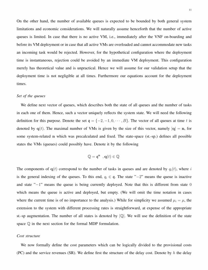
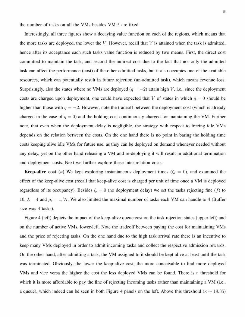
Figure 4 (left) depicts the impact of the keep-alive queue cost on the task rejection states (upper left) and

on the number of active VMs, lower-left. Note the tradeoff between paying the cost for maintaining VMs

and the price of rejecting tasks. On the one hand due to the high task arrival rate there is an incentive to

keep many VMs deployed in order to admit incoming tasks and collect the respective admission rewards.

On the other hand, after admitting a task, the VM assigned to it should be kept alive at least until the task

was terminated. Obviously, the lower the keep-alive cost, the more conceivable to find more deployed

VMs and vice versa the higher the cost the less deployed VMs can be found. There is a threshold for

which it is more affordable to pay the fine of rejecting incoming tasks rather than maintaining a VM (i.e.,

a queue), which indeed can be seen in both Figure 4 panels on the left. Above this threshold (κ ∼ 19.35)

19

Fig. 4. Left - Impact of the allocated VM cost. The upper graph shows the number of rejecting states. The lower graph shows howthe number of active queues is being reduced with the cost of having an allocated VM.Right - Impact of the delay cost.

all states lead to reject policy and there are no active VMs. Note that deploying a VM due to temporal

congestion can result in paying the price of maintaining an excessive number of unutilized VMs for a long

time period, especially when migration of tasks between VMs is not supported. Accordingly, the decision

maker should balance between the number of active VMs and the tasks arrival rate which is reflected by

the load. Specifically, when the keep alive cost is high, the decision maker should try to maintain less yet

congested VMs, at the price of rejecting a task once in a while. Indeed, as can be seen in the figure, the

decline from keeping all VMs alive and keeping no VMs alive is not strict and there is a keep-alive cost

range at which the number of deployed VMs gradually declined from all to no deployed VMs. Note that

the decline from 3 deployed VMs to 2 and later to 1 or zero was much sharper than the slope between

4 to 3 deployed VMs.

Delay cost (h) Next we examined the cost delaying tasks (Figures 4 (right)). Note the tradeoff, on the

one hand in order to keep delay low, one needs to preserve many active VMs and distribute the load among

them. On the other hand, preserving many active VMs results in high keep-alive cost. The arrival intensity

was 4.75 and µi = 1,∀i. The buffer size of each queue was 6. We set the keep-alive cost to 1. Rejecting fine

was set to 10. The delay constants we utilized were η1 = 1, η2 = 1.8, η3 = 2.5, η4 = 3.5, η5 = 4.5, η6 = 5.5,

for having 1, 2, 3, 4, 5 and 6 operational tasks on a VM, respectively. Figure 4 panels on the right depict

the average number of managed tasks (upper) and the number of rejected states (lower). Figures 4. Observe

20

that the number of rejecting states approached 100% of all states at highest values of h.

Since throughout this simulation setup, the keep-alive cost was sufficiently low compared to the

admission gain (i.e., no significant keep-alive to delay tradeoff), all the VMs were active. As expected,

the scheduler balanced between the loads of the operating VMs (as anticipated by the cost model in

Equation (1)). Expectedly, as long as the delaying costs were low, most of the tasks were admitted,

and very few states were rejecting states. When the delay cost increased, keeping several tasks on a VM

degraded the performance (the admission gain of a single task was lower than the extra delay cost incurred

by all tasks on the designated VM). When the delay cost was sufficiently high (around 1.8) having more

than one task per VM was costly, hence we could see only 4 operational tasks, one per VM. Note that

the interval of keeping a single task per VM was quite large, since the delay cost when a single task was

operational on a VM (η1) was low. When the delay cost was high enough (around 15) the admission gain

could not cover the task maintenance costs and all tasks were declined.

We inspected many other parameters analyzing the tradeoffs between different costs, searching for

threshold policy, and trying to understand the interdependencies between parameters. For example, a

threshold policy can be observed with respect to the deployment and termination of VMs as a function of

several parameters and their interdependencies. For example, if β and/or ψ are high compared to keep-

alive cost, the optimal policy acts to leave all queues active, even if empty. Clearly, the set of system

parameters and most importantly their proportional relation will determine the optimal policy, e.g., will

determine whether to admit or reject tasks, whether load balance between VMs to reduce the delay or to

shift loads to less VMs in order to release a VM, etc. However, due to space limitations we only provide

a sample of our results and only a glimpse at few observations, to exemplify the scheme usage.

B. Impact of VM time deployment - the ζi > 0 case

After ignoring the deployment delay, assuming that VMs can be deployed and terminated instanta-

neously, in this subsection we explored the effect of deployment delays. Obviously, the time which takes

to activate and inactivate VMs can have a major effect on the policy.

In practice, the length of this period depends on several aspects including the type of the machine.

For example, the applications which we dispatched for the execution on AWS in our implementation

(Section VI) were deployed and run on VMs of type ”tx4.large”. These VMs normally took between half

a minute and two minutes to deploy and boot the image. We repeated the numerical evaluation utilizing

21

the same parameters as before, varying the deployment delay (ζ). Note that ζ , in our notation, stands for

the rate (i.e., the reciprocal of the time).

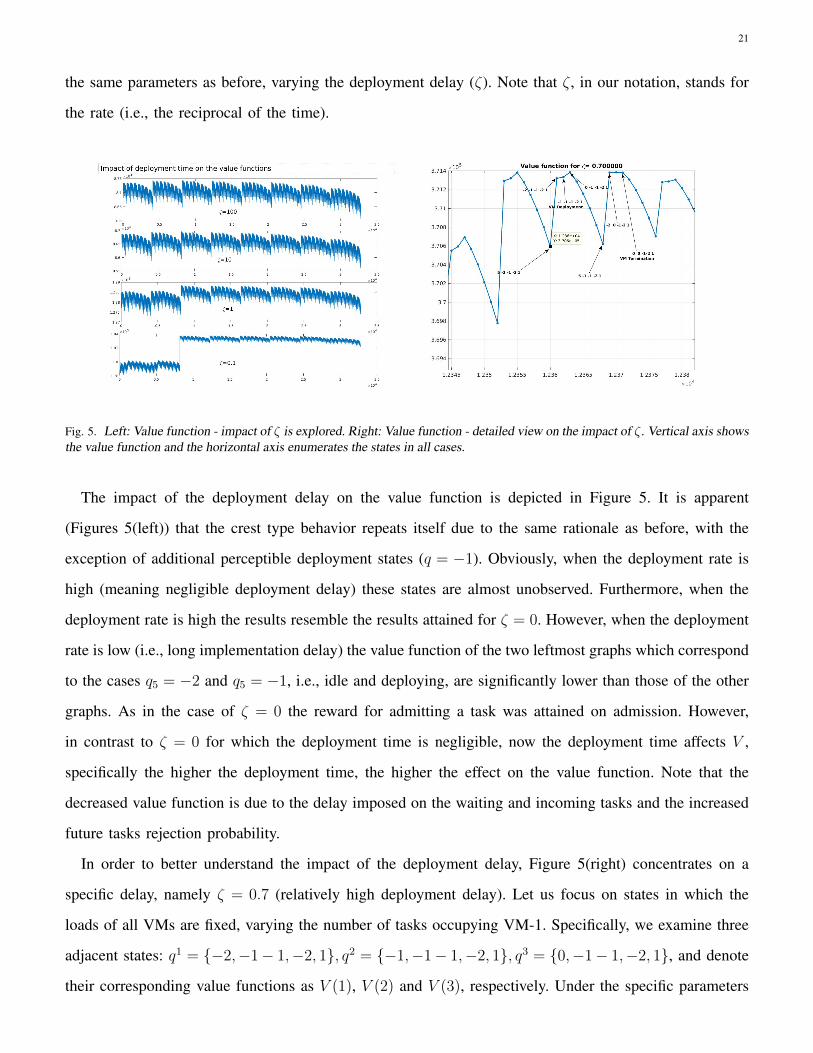
Fig. 5. Left: Value function - impact of ζ is explored. Right: Value function - detailed view on the impact of ζ. Vertical axis showsthe value function and the horizontal axis enumerates the states in all cases.

The impact of the deployment delay on the value function is depicted in Figure 5. It is apparent

(Figures 5(left)) that the crest type behavior repeats itself due to the same rationale as before, with the

exception of additional perceptible deployment states (q = −1). Obviously, when the deployment rate is

high (meaning negligible deployment delay) these states are almost unobserved. Furthermore, when the

deployment rate is high the results resemble the results attained for ζ = 0. However, when the deployment

rate is low (i.e., long implementation delay) the value function of the two leftmost graphs which correspond

to the cases q5 = −2 and q5 = −1, i.e., idle and deploying, are significantly lower than those of the other

graphs. As in the case of ζ = 0 the reward for admitting a task was attained on admission. However,

in contrast to ζ = 0 for which the deployment time is negligible, now the deployment time affects V ,

specifically the higher the deployment time, the higher the effect on the value function. Note that the

decreased value function is due to the delay imposed on the waiting and incoming tasks and the increased

future tasks rejection probability.

In order to better understand the impact of the deployment delay, Figure 5(right) concentrates on a

specific delay, namely ζ = 0.7 (relatively high deployment delay). Let us focus on states in which the

loads of all VMs are fixed, varying the number of tasks occupying VM-1. Specifically, we examine three

adjacent states: q1 = {−2,−1− 1,−2, 1}, q2 = {−1,−1− 1,−2, 1}, q3 = {0,−1− 1,−2, 1}, and denote

their corresponding value functions as V (1), V (2) and V (3), respectively. Under the specific parameters

22

(and specifically deployment and arrival rates and , especially their ratio), V of having a deployed VM

and despite the keep-alive cost, is higher than V where VM is inactive. The marginal difference between

states that have VM under deployment (q2 ) and inactive (q1) is smaller compared to the difference

between q3 (idle VM) and q2 (under deployment). That is, V (3)− V (2) > V (2)− V (1), indicating that

the advantage of having a pending request for VM deployment was less valuable than that of having

an already deployed empty queue, once ζ is small. Note that V (2) − V (1) captures the value of taking

the decision of VM deployment. As before, the more loaded the VMs, the lower the value; for example

the value of state {1,−1 − 1,−2, 1}, in which a single task occupies VM-1, is lower than that of state

{0,−1,−1,−2, 1} in which VM-1 is deployed but idle. More radical changes can be seen between V

of state {5,−1,−1,−2, 1}, in which VM-1 is fully loaded, and that of state {0,−2,−1,−2, 1}. Recall

that the reward for all the extra admitted tasks has already been obtained on admission. For comparison,

observe the three adjacent states q4 = {−2, 0− 1,−2, 1}, q5 = {−1, 0− 1,−2, 1}, q6 = {0, 0− 1,−2, 1},

which are different from the previous triplet by that the second VM state changed from −1 to 0, i.e.,

having VM-2 deployed idle and disposed to accept new tasks. Obviously, the need for a ready unloaded

VM now is less acute than before, i.e., the marginal contribution of an additional ready VM is less acute

than before. Indeed, as is apparent in the figure, there is no real value difference between the three states.

Further, their value function is even slightly lower than V of state q3, i.e., the implementation of a VM

when there is already an idle VM ready to accept tasks slightly degrades the value function due to the

expected keep-alive costs. Following the decision mechanism one can see that indeed VM q65 is marked

for termination if its only packet is served and it becomes empty before any other event. (recall that

decisions are taken only as a consequence of an event hence the VM termination must be triggered by a

service completion event and cannot be done afterwords then the queue was already empty).

C. Threshold-type structure of the optimal policy

In this subsection we give some insight into finding optimal policies (policies that maximize the expected

utility). In particular, we concentrate on the structure of the optimal policies trying to define thresholds

such that below such a threshold the system takes one action while above it, it takes a different action.

For example, the decision maker keeps admitting tasks to a VM only below a number of tasks occupying

this VM and above this threshold it will either assign new incoming tasks to a different VM (possibly

new one) or reject them. The motivation for identifying threshold policies stems from the fact that on

23

many systems, and in particular queueing systems, threshold policies are optimal or nearly optimal. We

mainly concentrate on actions which result in the deployment or termination of a VM and on the load

balancing policy on which VM to place an admitted task.

In order to define threshold policy, we first define state domination. Consider two states a and b, with

queue vectors denoted by qa and qb.

Definition 5.2 (State domination).

We define that state a dominates state b if and only if states a and b have the same number of idle, deployed and under

deployment queues, and qai ≥ qbi , ∀qai > 0, i ∈ {1, . . . ,n}. We denote such domination by qa � qb.

The following defines thresholds in build (VM deployment), scheduling, and destroy (VM termination):

Definition 5.3 (Threshold policies).

• Optimal threshold policy πb exists if a deployment of previously inactive VM at state qa means deployment is also optimal

at all states qb such that qb � qa

• Optimal threshold policy πd exists if an optimal termination queue at state qa means termination is also optimal at all

states qb such that qa � qb.

• Optimal threshold policy πu exists if the optimal load balancing policy in state qa is the same as the optimal scheduling

policy for all states qb such that qb � qa and qbi = qai .

We identify the existence of threshold policies both by observation and by using the following analytical

result which states the monotonicity of the value function:

Lemma 5.1 (Value function domination). For any qa � qb it holds V (qa) ≤ V (qb).

The intuition behind this Lemma is quite straightforward; as previously explained, the reward for

admitting a task was attained on admission, hence after admitting a task, it is only a burden on the value

function, hence the more tasks are present in a VM the lower the value. This monotonicity is clearly

depicted in Figure 5(right). For example, the four states to the left of state {5,−1,−1,−2, 1} which

correspond to states {4,−1,−1,−2, 1},{3,−1,−1,−2, 1},{2,−1,−1,−2, 1} and {1,−1,−1,−2, 1} have

a decreasing number of tasks on VM-1 and the same number of tasks on all other active VMs, their value

gradually increased accordingly. The formal proof to Lemma 5.1 appears in Appendix C.

Lemma 5.1 analytically states a structural property of the value function, which suggests the existence

of threshold policy. Next we illustrate these threshold policies on our numerical results. Note that these

threshold policies coincide with the general intuition previously explained. In particular, since the action

b is motivated by the intention to reduce future costs due to the loads on the active VMs which include

24

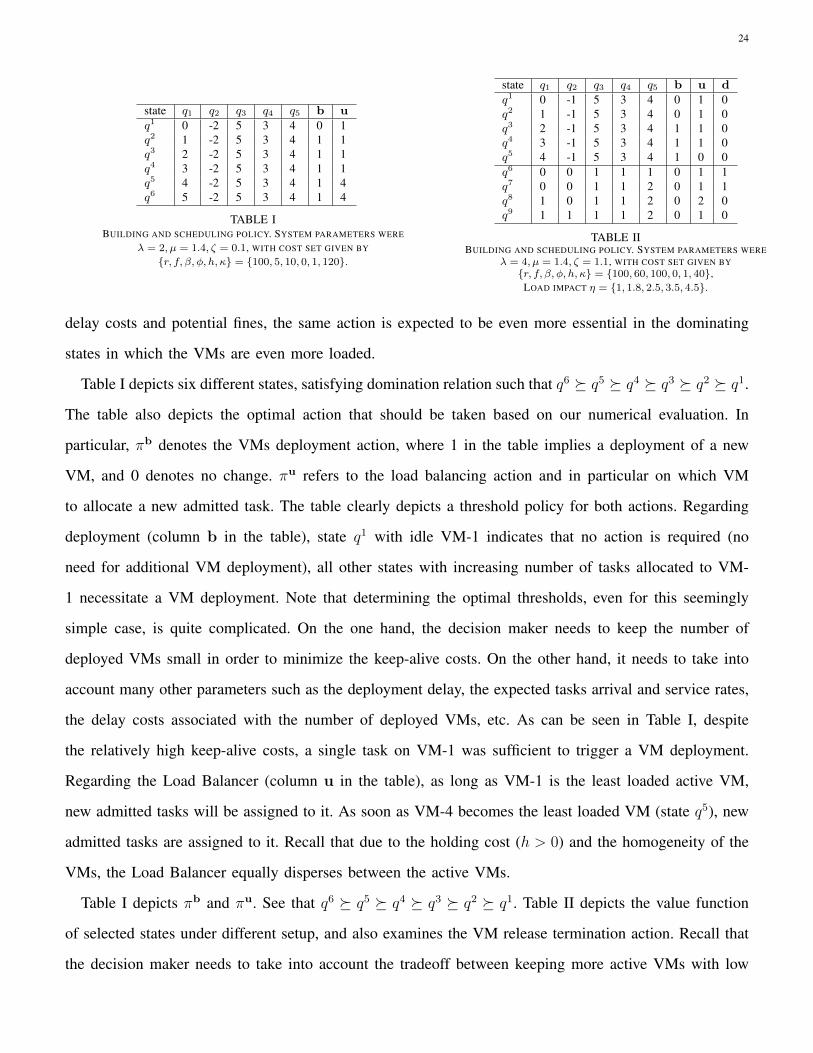
state q1 q2 q3 q4 q5 b uq1 0 -2 5 3 4 0 1q2 1 -2 5 3 4 1 1q3 2 -2 5 3 4 1 1q4 3 -2 5 3 4 1 1q5 4 -2 5 3 4 1 4q6 5 -2 5 3 4 1 4

TABLE IBUILDING AND SCHEDULING POLICY. SYSTEM PARAMETERS WERE

λ = 2, µ = 1.4, ζ = 0.1, WITH COST SET GIVEN BY

{r, f, β, φ, h, κ} = {100, 5, 10, 0, 1, 120}.

state q1 q2 q3 q4 q5 b u dq1 0 -1 5 3 4 0 1 0q2 1 -1 5 3 4 0 1 0q3 2 -1 5 3 4 1 1 0q4 3 -1 5 3 4 1 1 0q5 4 -1 5 3 4 1 0 0q6 0 0 1 1 1 0 1 1q7 0 0 1 1 2 0 1 1q8 1 0 1 1 2 0 2 0q9 1 1 1 1 2 0 1 0

TABLE IIBUILDING AND SCHEDULING POLICY. SYSTEM PARAMETERS WERE

λ = 4, µ = 1.4, ζ = 1.1, WITH COST SET GIVEN BY{r, f, β, φ, h, κ} = {100, 60, 100, 0, 1, 40},

LOAD IMPACT η = {1, 1.8, 2.5, 3.5, 4.5}.

delay costs and potential fines, the same action is expected to be even more essential in the dominating

states in which the VMs are even more loaded.

Table I depicts six different states, satisfying domination relation such that q6 � q5 � q4 � q3 � q2 � q1.

The table also depicts the optimal action that should be taken based on our numerical evaluation. In

particular, πb denotes the VMs deployment action, where 1 in the table implies a deployment of a new

VM, and 0 denotes no change. πu refers to the load balancing action and in particular on which VM

to allocate a new admitted task. The table clearly depicts a threshold policy for both actions. Regarding

deployment (column b in the table), state q1 with idle VM-1 indicates that no action is required (no

need for additional VM deployment), all other states with increasing number of tasks allocated to VM-

1 necessitate a VM deployment. Note that determining the optimal thresholds, even for this seemingly

simple case, is quite complicated. On the one hand, the decision maker needs to keep the number of

deployed VMs small in order to minimize the keep-alive costs. On the other hand, it needs to take into

account many other parameters such as the deployment delay, the expected tasks arrival and service rates,

the delay costs associated with the number of deployed VMs, etc. As can be seen in Table I, despite

the relatively high keep-alive costs, a single task on VM-1 was sufficient to trigger a VM deployment.

Regarding the Load Balancer (column u in the table), as long as VM-1 is the least loaded active VM,

new admitted tasks will be assigned to it. As soon as VM-4 becomes the least loaded VM (state q5), new

admitted tasks are assigned to it. Recall that due to the holding cost (h > 0) and the homogeneity of the

VMs, the Load Balancer equally disperses between the active VMs.

Table I depicts πb and πu. See that q6 � q5 � q4 � q3 � q2 � q1. Table II depicts the value function

of selected states under different setup, and also examines the VM release termination action. Recall that

the decision maker needs to take into account the tradeoff between keeping more active VMs with low

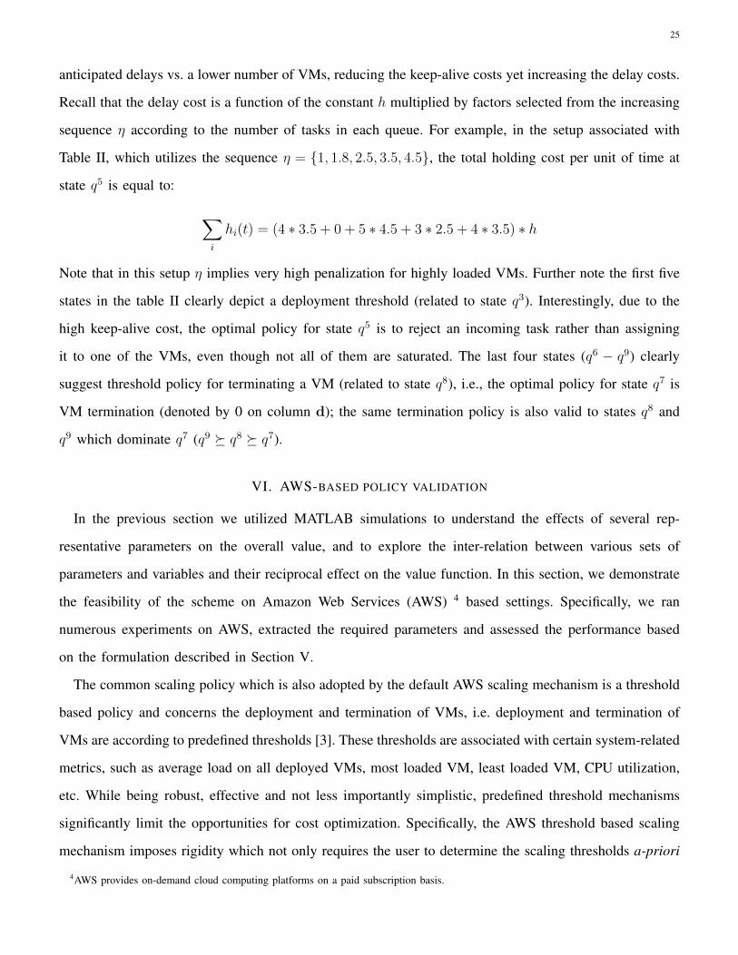
25

anticipated delays vs. a lower number of VMs, reducing the keep-alive costs yet increasing the delay costs.

Recall that the delay cost is a function of the constant h multiplied by factors selected from the increasing

sequence η according to the number of tasks in each queue. For example, in the setup associated with

Table II, which utilizes the sequence η = {1, 1.8, 2.5, 3.5, 4.5}, the total holding cost per unit of time at

state q5 is equal to:

∑i

hi(t) = (4 ∗ 3.5 + 0 + 5 ∗ 4.5 + 3 ∗ 2.5 + 4 ∗ 3.5) ∗ h

Note that in this setup η implies very high penalization for highly loaded VMs. Further note the first five

states in the table II clearly depict a deployment threshold (related to state q3). Interestingly, due to the

high keep-alive cost, the optimal policy for state q5 is to reject an incoming task rather than assigning

it to one of the VMs, even though not all of them are saturated. The last four states (q6 − q9) clearly

suggest threshold policy for terminating a VM (related to state q8), i.e., the optimal policy for state q7 is

VM termination (denoted by 0 on column d); the same termination policy is also valid to states q8 and

q9 which dominate q7 (q9 � q8 � q7).

VI. AWS-BASED POLICY VALIDATION

In the previous section we utilized MATLAB simulations to understand the effects of several rep-

resentative parameters on the overall value, and to explore the inter-relation between various sets of

parameters and variables and their reciprocal effect on the value function. In this section, we demonstrate

the feasibility of the scheme on Amazon Web Services (AWS) 4 based settings. Specifically, we ran

numerous experiments on AWS, extracted the required parameters and assessed the performance based

on the formulation described in Section V.

The common scaling policy which is also adopted by the default AWS scaling mechanism is a threshold

based policy and concerns the deployment and termination of VMs, i.e. deployment and termination of

VMs are according to predefined thresholds [3]. These thresholds are associated with certain system-related

metrics, such as average load on all deployed VMs, most loaded VM, least loaded VM, CPU utilization,

etc. While being robust, effective and not less importantly simplistic, predefined threshold mechanisms

significantly limit the opportunities for cost optimization. Specifically, the AWS threshold based scaling

mechanism imposes rigidity which not only requires the user to determine the scaling thresholds a-priori

4AWS provides on-demand cloud computing platforms on a paid subscription basis.

26

but more importantly provides no scaling tools which respond according to the detailed states of each VM,

hence limits the range of attainable solution. Furthermore, even though the AWS threshold based scaling

mechanism provides a wide range of flexibility, allowing the user to program its own thresholds a-priori,

it restricts the thresholds to rely on the system parameters available through the AWS console (which

represent maximum or average load for all active VMs), highly limiting the users flexibility. Both reasons

prevented us from deploying the complete suggested scheme on AWS and forced us to utilize a hybrid

scheme which interlace the AWS platform with adjacent offline Matlab value-computations. Specifically,

throughout this section we rely on qualitative validation, i.e., we extract all system states, parameters,

statistics and performance values in real-time from AWS throughout each evaluation test, yet the eventual

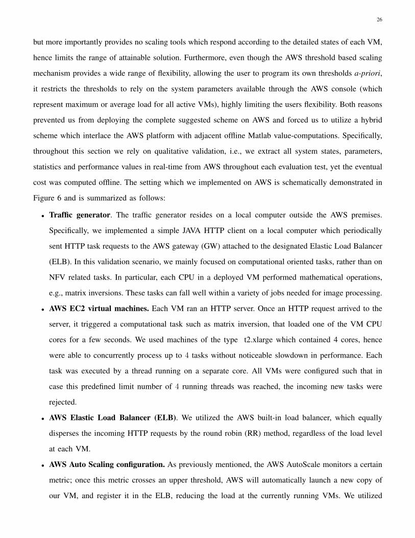
cost was computed offline. The setting which we implemented on AWS is schematically demonstrated in

Figure 6 and is summarized as follows:

• Traffic generator. The traffic generator resides on a local computer outside the AWS premises.

Specifically, we implemented a simple JAVA HTTP client on a local computer which periodically

sent HTTP task requests to the AWS gateway (GW) attached to the designated Elastic Load Balancer

(ELB). In this validation scenario, we mainly focused on computational oriented tasks, rather than on

NFV related tasks. In particular, each CPU in a deployed VM performed mathematical operations,

e.g., matrix inversions. These tasks can fall well within a variety of jobs needed for image processing.

• AWS EC2 virtual machines. Each VM ran an HTTP server. Once an HTTP request arrived to the

server, it triggered a computational task such as matrix inversion, that loaded one of the VM CPU

cores for a few seconds. We used machines of the type t2.xlarge which contained 4 cores, hence

were able to concurrently process up to 4 tasks without noticeable slowdown in performance. Each

task was executed by a thread running on a separate core. All VMs were configured such that in

case this predefined limit number of 4 running threads was reached, the incoming new tasks were

rejected.

• AWS Elastic Load Balancer (ELB). We utilized the AWS built-in load balancer, which equally

disperses the incoming HTTP requests by the round robin (RR) method, regardless of the load level

at each VM.

• AWS Auto Scaling configuration. As previously mentioned, the AWS AutoScale monitors a certain

metric; once this metric crosses an upper threshold, AWS will automatically launch a new copy of

our VM, and register it in the ELB, reducing the load at the currently running VMs. We utilized

27

average CPU load as our metric for the upper threshold. The Auto Scaling configuration also specifies

the maximal number of VMs and the thresholds for opening/closing a VM; it includes cloud-watch

alarms which signal to deploy or to terminate a VM according to the policy. Each VM also listened

on another port for ”keep alive messages” from the ELB.

Fig. 6. AWS validation set-up scheme

As previously mentioned, AWS scaling mech-

anism relies on threshold based policy, i.e., a

user can control when to scale-in or scale-out by

choosing one or more system parameters (e.g.,

load) and by determining a threshold according

to these system parameters for deployment and

termination of VMs. As was shown in previous

sections by observation of numerical results, the optimal policy disclosed by the MDP is a threshold

based policy (at least with respect to some of the parameters examined). Accordingly, our objective

was to understand the effect of these threshold values on the value attained, and to compare it with

the optimal thresholds attained by the MDP formulation. In order to evaluate the values attained by

each set of thresholds experimentally, and in order to formulate the MDP and solve the corresponding

Bellman equation for determining the optimal value analytically, we need to acquire the required system

parameters. For example, we need to know the effect of task loads on the performance, i.e., to acquire

the statistical properties of task processing-time-distribution under different VM load levels, we need to

obtain VM deployment time, etc. This data was extracted by the AWS Cloud-Watch mechanism throughout

each experiment and fed back to the MDP formulation. We evaluated the system under moderate traffic

intensity (Arrivals were about 300 tasks per hour, while service rates at each VM were about 50 tasks

per hour). The AWS VM deployment and termination thresholds were set with respect to CPU utilization

(i.e., the average CPU utilization on all deployed VMs), examining the effect of various thresholds for

deploying (scale-out) and discharging (scale-in) VMs, on the value function. Each pair of thresholds was

examined for a long duration to get sufficient statistics, extracting all the required system parameters.

The associated values were computed offline based on the collected traces. Since the main goal of this

deployment is a proof of concept, and due to budget constraints, we examined only several thresholds.

The set of coupled threshold values examined are given in Table III. For tractability we indexed the

paired values from 1 to 12 (e.g., pair number 4 denotes 40% CPU-utilization and 60% CPU-utilization for

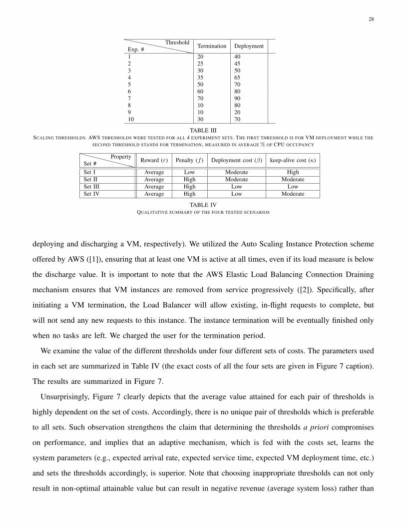
28

``````````Exp. #Threshold Termination Deployment

1 20 402 25 453 30 504 35 655 50 706 60 807 70 908 10 809 10 2010 30 70

TABLE IIISCALING THRESHOLDS. AWS THRESHOLDS WERE TESTED FOR ALL 4 EXPERIMENT SETS. THE FIRST THRESHOLD IS FOR VM DEPLOYMENT WHILE THE

SECOND THRESHOLD STANDS FOR TERMINATION, MEASURED IN AVERAGE % OF CPU OCCUPANCY

XXXXXXXXXSet #Property Reward (r) Penalty (f ) Deployment cost (β) keep-alive cost (κ)

Set I Average Low Moderate HighSet II Average High Moderate ModerateSet III Average High Low LowSet IV Average High Low Moderate

TABLE IVQUALITATIVE SUMMARY OF THE FOUR TESTED SCENARIOS

deploying and discharging a VM, respectively). We utilized the Auto Scaling Instance Protection scheme

offered by AWS ([1]), ensuring that at least one VM is active at all times, even if its load measure is below

the discharge value. It is important to note that the AWS Elastic Load Balancing Connection Draining

mechanism ensures that VM instances are removed from service progressively ([2]). Specifically, after

initiating a VM termination, the Load Balancer will allow existing, in-flight requests to complete, but

will not send any new requests to this instance. The instance termination will be eventually finished only

when no tasks are left. We charged the user for the termination period.

We examine the value of the different thresholds under four different sets of costs. The parameters used

in each set are summarized in Table IV (the exact costs of all the four sets are given in Figure 7 caption).

The results are summarized in Figure 7.

Unsurprisingly, Figure 7 clearly depicts that the average value attained for each pair of thresholds is

highly dependent on the set of costs. Accordingly, there is no unique pair of thresholds which is preferable

to all sets. Such observation strengthens the claim that determining the thresholds a priori compromises

on performance, and implies that an adaptive mechanism, which is fed with the costs set, learns the

system parameters (e.g., expected arrival rate, expected service time, expected VM deployment time, etc.)

and sets the thresholds accordingly, is superior. Note that choosing inappropriate thresholds can not only

result in non-optimal attainable value but can result in negative revenue (average system loss) rather than

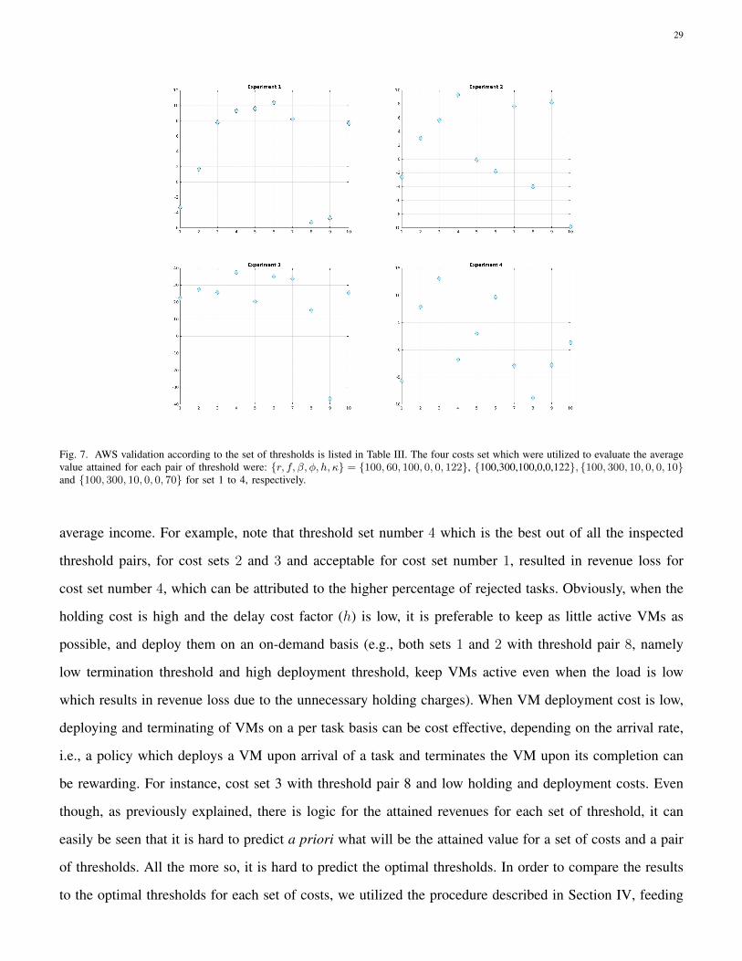
29

Fig. 7. AWS validation according to the set of thresholds is listed in Table III. The four costs set which were utilized to evaluate the averagevalue attained for each pair of threshold were: {r, f, β, φ, h, κ} = {100, 60, 100, 0, 0, 122}, {100,300,100,0,0,122}, {100, 300, 10, 0, 0, 10}and {100, 300, 10, 0, 0, 70} for set 1 to 4, respectively.

average income. For example, note that threshold set number 4 which is the best out of all the inspected

threshold pairs, for cost sets 2 and 3 and acceptable for cost set number 1, resulted in revenue loss for

cost set number 4, which can be attributed to the higher percentage of rejected tasks. Obviously, when the

holding cost is high and the delay cost factor (h) is low, it is preferable to keep as little active VMs as

possible, and deploy them on an on-demand basis (e.g., both sets 1 and 2 with threshold pair 8, namely

low termination threshold and high deployment threshold, keep VMs active even when the load is low

which results in revenue loss due to the unnecessary holding charges). When VM deployment cost is low,

deploying and terminating of VMs on a per task basis can be cost effective, depending on the arrival rate,

i.e., a policy which deploys a VM upon arrival of a task and terminates the VM upon its completion can

be rewarding. For instance, cost set 3 with threshold pair 8 and low holding and deployment costs. Even

though, as previously explained, there is logic for the attained revenues for each set of threshold, it can

easily be seen that it is hard to predict a priori what will be the attained value for a set of costs and a pair

of thresholds. All the more so, it is hard to predict the optimal thresholds. In order to compare the results

to the optimal thresholds for each set of costs, we utilized the procedure described in Section IV, feeding

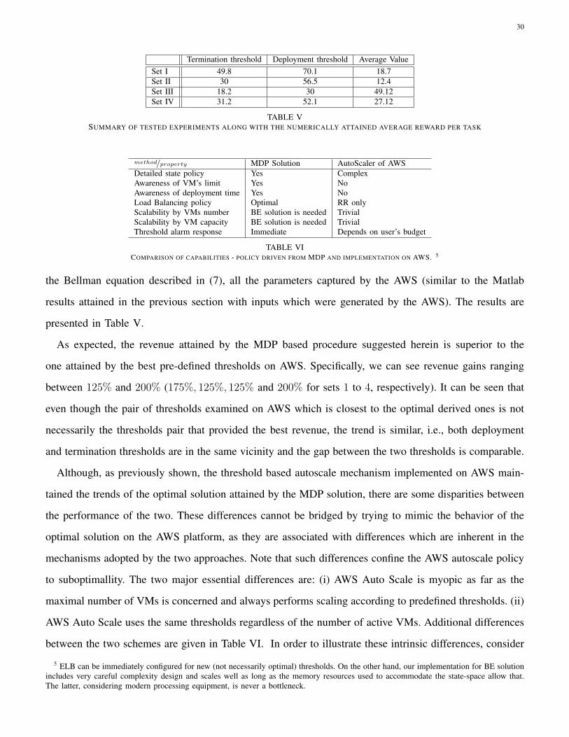
30

Termination threshold Deployment threshold Average ValueSet I 49.8 70.1 18.7Set II 30 56.5 12.4Set III 18.2 30 49.12Set IV 31.2 52.1 27.12

TABLE VSUMMARY OF TESTED EXPERIMENTS ALONG WITH THE NUMERICALLY ATTAINED AVERAGE REWARD PER TASK

method/property MDP Solution AutoScaler of AWSDetailed state policy Yes ComplexAwareness of VM’s limit Yes NoAwareness of deployment time Yes NoLoad Balancing policy Optimal RR onlyScalability by VMs number BE solution is needed TrivialScalability by VM capacity BE solution is needed TrivialThreshold alarm response Immediate Depends on user’s budget

TABLE VICOMPARISON OF CAPABILITIES - POLICY DRIVEN FROM MDP AND IMPLEMENTATION ON AWS. 5

the Bellman equation described in (7), all the parameters captured by the AWS (similar to the Matlab

results attained in the previous section with inputs which were generated by the AWS). The results are

presented in Table V.

As expected, the revenue attained by the MDP based procedure suggested herein is superior to the

one attained by the best pre-defined thresholds on AWS. Specifically, we can see revenue gains ranging

between 125% and 200% (175%, 125%, 125% and 200% for sets 1 to 4, respectively). It can be seen that

even though the pair of thresholds examined on AWS which is closest to the optimal derived ones is not

necessarily the thresholds pair that provided the best revenue, the trend is similar, i.e., both deployment

and termination thresholds are in the same vicinity and the gap between the two thresholds is comparable.

Although, as previously shown, the threshold based autoscale mechanism implemented on AWS main-

tained the trends of the optimal solution attained by the MDP solution, there are some disparities between

the performance of the two. These differences cannot be bridged by trying to mimic the behavior of the

optimal solution on the AWS platform, as they are associated with differences which are inherent in the

mechanisms adopted by the two approaches. Note that such differences confine the AWS autoscale policy

to suboptimallity. The two major essential differences are: (i) AWS Auto Scale is myopic as far as the

maximal number of VMs is concerned and always performs scaling according to predefined thresholds. (ii)

AWS Auto Scale uses the same thresholds regardless of the number of active VMs. Additional differences

between the two schemes are given in Table VI. In order to illustrate these intrinsic differences, consider

5 ELB can be immediately configured for new (not necessarily optimal) thresholds. On the other hand, our implementation for BE solutionincludes very careful complexity design and scales well as long as the memory resources used to accommodate the state-space allow that.The latter, considering modern processing equipment, is never a bottleneck.

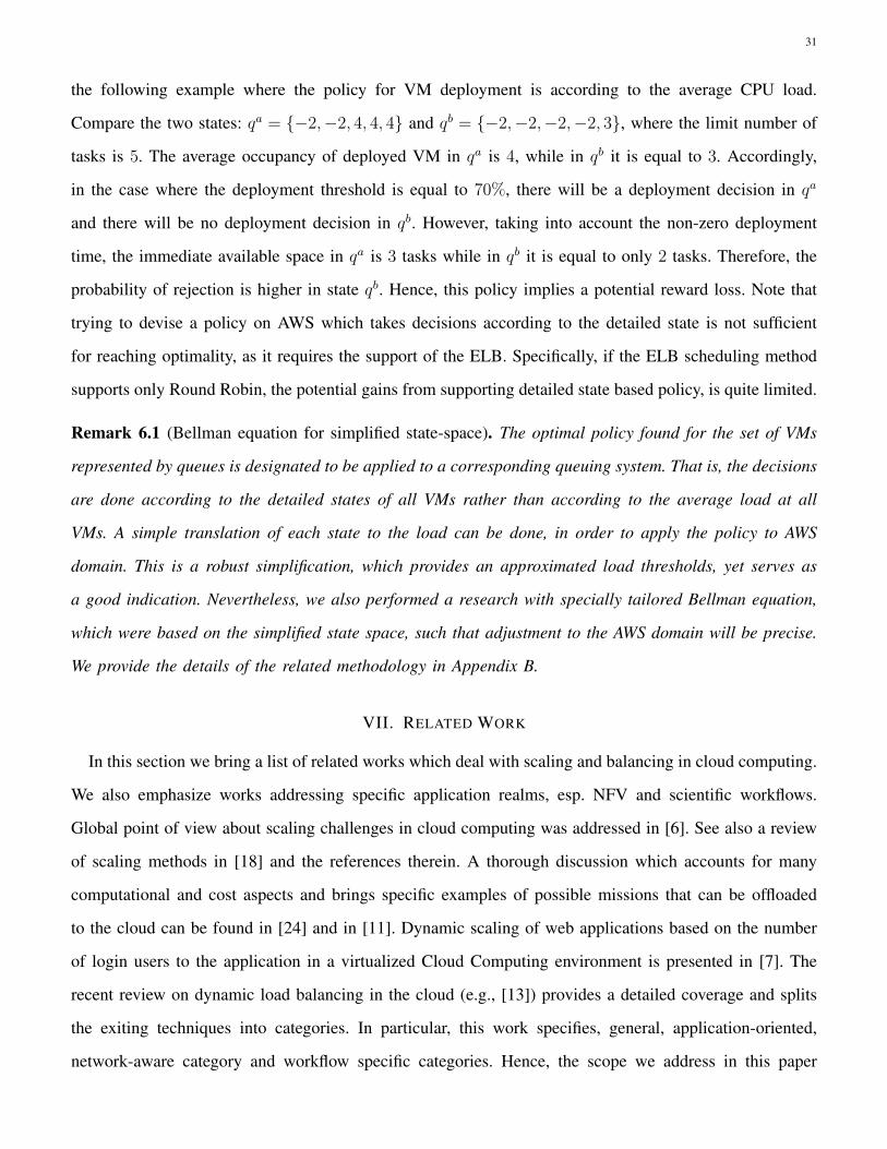
31

the following example where the policy for VM deployment is according to the average CPU load.

Compare the two states: qa = {−2,−2, 4, 4, 4} and qb = {−2,−2,−2,−2, 3}, where the limit number of

tasks is 5. The average occupancy of deployed VM in qa is 4, while in qb it is equal to 3. Accordingly,

in the case where the deployment threshold is equal to 70%, there will be a deployment decision in qa

and there will be no deployment decision in qb. However, taking into account the non-zero deployment

time, the immediate available space in qa is 3 tasks while in qb it is equal to only 2 tasks. Therefore, the

probability of rejection is higher in state qb. Hence, this policy implies a potential reward loss. Note that

trying to devise a policy on AWS which takes decisions according to the detailed state is not sufficient

for reaching optimality, as it requires the support of the ELB. Specifically, if the ELB scheduling method

supports only Round Robin, the potential gains from supporting detailed state based policy, is quite limited.

Remark 6.1 (Bellman equation for simplified state-space). The optimal policy found for the set of VMs

represented by queues is designated to be applied to a corresponding queuing system. That is, the decisions

are done according to the detailed states of all VMs rather than according to the average load at all

VMs. A simple translation of each state to the load can be done, in order to apply the policy to AWS

domain. This is a robust simplification, which provides an approximated load thresholds, yet serves as

a good indication. Nevertheless, we also performed a research with specially tailored Bellman equation,

which were based on the simplified state space, such that adjustment to the AWS domain will be precise.

We provide the details of the related methodology in Appendix B.

VII. RELATED WORK

In this section we bring a list of related works which deal with scaling and balancing in cloud computing.

We also emphasize works addressing specific application realms, esp. NFV and scientific workflows.

Global point of view about scaling challenges in cloud computing was addressed in [6]. See also a review

of scaling methods in [18] and the references therein. A thorough discussion which accounts for many

computational and cost aspects and brings specific examples of possible missions that can be offloaded

to the cloud can be found in [24] and in [11]. Dynamic scaling of web applications based on the number

of login users to the application in a virtualized Cloud Computing environment is presented in [7]. The

recent review on dynamic load balancing in the cloud (e.g., [13]) provides a detailed coverage and splits

the exiting techniques into categories. In particular, this work specifies, general, application-oriented,

network-aware category and workflow specific categories. Hence, the scope we address in this paper

32

is highly relevant. Challenges of VNF scheduling by means of software-defined networks (SDN) were

introduced in [23]. Technical details of how the VNF could be deployed are discussed in [25]. Integration

of NFV and SDN was also addressed in [9] in the context of 5G mobile core networks. In [33], joint

optimization of NFVI resources under multiple constraints results in approximate algorithm which aims

at improving the capability of NFV management and orchestration. This work provides static placement

of NFV-related resource. Near optimal NP-hard placement problem is approximately solved by linear

algorithm in [8]. The problem of VNF scheduling aimed to optimize performance latency, was treated by

linear programming in [22].

Offloading scientific workflows to a cloud have recently received intensive attention, see, e.g., [34],[15],[17].

Specific examples include but not limited to cloud-based Neural Networks [27], processing of astronomy

data [30], e-business workflows [32].

Some of the following works in queuing control can be seen as potentially applied to cloud computing.

In [19], queue scheduling algorithm named 2DFQ separates requests with different costs and different size

across different worker threads. It also extends to the case where the costs are variable or unpredictable.

Optimal scheduling in hybrid cloud environment was studied in [26]. The solution provided by the authors

employs MDP as well. A great deal of work provides joint results on queue scheduling and optimization.

We mention works which deal with fixed number of queues or queue networks, e.g. [29], [20], [10] and

works which take this number to the limit, e.g. [12], [14], [21]. See also and references therein. This work,

in contrary, treat the specific scenario, where the number of queues is finite but flexible, incorporating

features of deployment cost and time and termination. Therefore, we developed a model which captures

all these features and treat it by MDP.

VIII. CONCLUSION

In this work, we presented a scaling and load balancing mechanism by means of optimal stochastic

control, in a complex setting where cloud users (applications) aim to optimize their overall costs. The

overall cost depends on several cost parameters which can be classified into two basic cost types. The first

one we categorize as service revenues which are associated with SLA, namely rewards for successfully

admitted tasks, fines for rejections and reward reduction for low performance. The second one we

categorize as provisional costs; these refer to the Operators expenditures towards the cloud provider;

they include cost of VM deployment and termination and cost of having VMs on-line (keep-alive cost).

The controlling agent which manages both the scaling procedure and the load balancing mechanism,

33

receive as inputs various Key Performance Indicators (KPIs) such as the load on each deployed VM,

and based on the anticipated loads, the expected performance and the set of costs determine whether to

deploy or terminate a VM, and to which VM to allocate an arrival task. For example, based on the system

state, expected load and related performance and the anticipated value (cost) the agent can decide to stop

diverting tasks to a specific VM in order to empty it and terminate its operation without dropping any

tasks on the way. We formulated the problem by Markov Decision Process and derived optimal policy

which optimized the applications total cost. The value function, the optimized cost and the optimal policy

(which is a direct product of it), were thoroughly investigated numerically. In particular, we numerically

explored the effect of various cost parameters (e.g., holding cost and task rejection penalty), operational

parameters (e.g., deployment and termination times), performance parameters (e.g., VMs load effect on

task latency) and their interdependence on the optimal policy. Via this comprehensive study, we derived

several important properties of the value functions and the corresponding policies. We further examined

threshold-type policies which are the common policy in operational deployments. Our work was validated

through implementation of several aspects on AWS, and extracting the relevant KPIs while operating

this Amazon cloud computing platform under various setups. Our results endorse, that even under this

limited platform, the policy found by operating the corresponding MDP procedure suggested in this paper

outperforms a-priori determined thresholds and can be utilized to determine a dynamic policy which reacts

according to the actual system state.

APPENDIX

A. Derivation of Bellman equation

For succinctness, we prove for the case where ζi = 0, ∀i. Note that we assume the deployments onlyoccur at arrivals, while terminations occur only at service completions. Write the cost function as follows:

J =

∫ ∞0

e−γt[(b(t) · β + u(t) · r − f ∗ (1−

q∑i

ui(t)))dA(t) +

(d(t) · ψdD(t)

)+

q∑i

(hi(t) + κ ∗ (1− Iii)

)dt],

where D(t) is a vector form of the departing processes {D(i)}. We take infinitesimal θ such that only oneor no event can happen (probability of more than one is negligible), and use the dynamic programmingprinciple.

J(q(0)) =

∫ θ

0

e−γt[(b(t) · β + u(t) · r − f ∗ (1−

q∑i

ui(t)))dA(t) +

(d(t) · ψdD(t)

)+

q∑i

(hi(t) + κ ∗ (1− Iii)

)dt]

+ e−γθJ(q(θ)) = Jθ + e−γθJ(q(θ)),

34

Expanding for all options of J(q(θ)) after the time θ we have:

Jθ + e−γθ[λθJ(q + u) +

q∑i

µJ(q − ei) + (1− λθ −q∑i

µ)J(q)]

(10)

We use the following derivation:

E∫ θ

0

e−γtdA(t) = λ

∫ θ

0

e−γtdt = λ1− e−γθ

γ= λθ, (11)

In what follows we use e−γθ ' 1 − γθ as θ → 0. Calculate first the time used for a service in theinfinitesimal interval [0, θ]. Ti(t) =

∫ θ0

(1− Ie(t))(1− Ii(t))dt. Next, denote the potential service time processwhich counts exponentially distributed service times as Si(t). Then, Di(t) = Si(Ti(t)). Hence, as long asinterval [0, θ] is small, write E

∫ θ0e−γtdDi(t) = (1− Ie)(1− Ii)µi = µi. Write the costs incurred in [0, θ]

Jθ = λθ(u · r − b · β − f(1−q∑i

ui))− µθ(d · ψ)− C(q)θ

We now turn to the second term of (10),

(1− γθ)[λθJ(q + u) +

q∑i

µJ(q − ei) + (1− λθ −n∑i

µ)J(q)]

multiply all sides by γ and mind that θ2 ' 0.

γJ(q) = γ(λθ(u · r − b · β − f(1−

q∑i

ui))− µθ(d · ψ)− C(q)θ)

+ γ(1− γθ)[λθJ(q + u)

+

q∑i

µθJ(q − ei) + (1− λθ −q∑i

µθ)J(q)]

= γ(λθ(u · r − b · β − f(1−

q∑i

ui))− µθ(d · ψ)

− C(q)θ)

+[λθγJ(q + u) +

q∑i

µθγJ(q − ei) + (γ − λθγ −q∑i

µθγ)J(q)− γθJ(q)]

See that γJ(q) on both sides cancels out and denote δq = (∑q

i µ+ λ+ γ)−1. Write:

γθδ−1q J(q) = γθ

(λ(u · r − b · β − f(1−

q∑i

ui))− µ(d · ψ)− C(q))

+ γθ[λJ(q + s) +

q∑i

µJ(q − ei)]

Divide all by γθ and multiply by δq

J(q) =(λ(u · r − b · β − f(1−

q∑i

ui))− µ(d · ψ)− C(q))δq +

[λJ(q + u) +

q∑i

µJ(q − ei)]δq

Arrange according to the processes:

J(q) = δqλ[u · r − b · β − f(1−

q∑i

ui) + J(q + u)]

+[ q∑

i

µJ(q − ei)− µ(d · ψ)]δq − C(q)δq

Observe that by definition, u,b,d incorporate (in corresponding feasible cases) the scheduling, build

and destroy decisions, respectively. Hence, this equation is identical to (5), where the feasibility is ensured

35

by the corresponding indicators.

B. Bellman equations for simplified state-spaces

We provide Bellman equations for simplified state-space, such that the optimal policy is directly derived

in terms of the average load on all VMs. Consider first a two dimensional state space denoted by S1,

such that S1 =M×L×Z , where

M = {1, · · · ,Mmax} ,Z = {1, · · · ,Mmax} and L = {0, l, 2l, · · · , Lmax}

Mmax denotes the maximal number of active VMs and L represents deployed VM utilization, i.e., L

denotes the average load on all active VMs in units of percentage of the maximal load. For instance, if

there is a single active VM which can accommodate up to 4 tasks, serving a single task, then L = 14

= 25%,

if there are three active VMs each potentially accommodating up to 4 tasks, serving altogether 6 tasks

(regardless of how many each one serves), the load is: L = 63×4 = 50%. Lmax corresponds to the maximal

load of 100%, and l is the resolution of the space L, which, for our purposes was chose to correspond to

5% or 10%. The spacesM and Z stand for the number of active and deploying (i.e., being in the process

of deployment but not yet ready to accept tasks) VMs. Clearly it holds Z + M ≤ Mmax. Note that the

minimal number of active VMs is set to 1, which corresponds to the AWS property of preserving at least

one active VM. Also note that VMs in the process of deployment are considered as active with zero load.

Recall that r and β denote the reward for admitted tasks and the deployment cost, respectively. Also

recall the notations for actions b and d, standing for deployment of a new VM and termination of a VM.Consider C(L,M,Z)), the cost per unit of time associated with having M active machines with average

load L and Z deploying machines. Observe that upon task service or admission the load does not necessar-ily increases or decreases by 1. Hence we introduce transition probabilities p((L′,M ′, Z ′)|(L,M,Z),b)

and p((L′,M ′, Z ′)|(L,M,Z),d). The straightforward method to obtain these probabilities and rewardC(L,M,Z)) for all states is by learning through simulating of the optimal policy for the original queuingsystem with the optimal policy for the full state-space. Once the learning is done the value function of

36

the simplified state-space can be calculated according to the following:

V (L,M,Z) =[C(L,M,Z) + λmax

b{∑L′

p((L′,M,Z)|(L,M,Z),b = 0)V (L′,M,Z) + r, (12)

∑L′

p((L′,M,Z + 1)|(L,M,Z),b = 1)V (L′,M,Z + 1) + r − β} (13)

+ ζL,M,ZV (L,M + 1, Z − 1) (14)

+ µL,M,Z max{∑L′

p((L′,M,Z)|(L,M,Z),d = 0)V (L′,M,Z), (15)

∑L′

p((L′,M − 1, Z)|(L,M,Z)d = 1)V (L′,M − 1, Z)}]δL,M,Z (16)

Note that the rates service rates µL,M,Z and VM deployment reciprocal time ζL,M,Z are learned within

the same learning process. In 12 and 13 the selection regarding opening a new VM is written. Part 14

refers to the new VM deployment process. The selection if to terminate a VM upon service completion

is written in 15 and 16. For the sake of succinctness, we omitted here the boundary conditions of the

Bellman equation above.

In order to further adjust to AWS limitations the space M and the space Z can be degenerated to

M = {0, 1}, Z = {0, 1} thus being agnostic to the number of deployed VMs and considering only the

information if the maximal number of VMs has been deployed or not and if there is a VM in deployment

process. In this case, the entire dynamics of the value function and the transition probabilities will be

solely expressed by the load.

C. Proof of Lemma 5.1

We show that for any qa � qb it holds V (qa) ≤ V (qb). Proof. To show the statement define two

systems, denoted by a and b. At time t the state of each system is denoted by at and bt. Next, we

stochastically couple these systems. Namely, we apply the same policy to both states, denoted as πab. The

policy is optimal for the system a, while system b mimics all actions from system a. In particular the

mimicking policy follows the following rules:

1) A task which is scheduled in a is scheduled in b into the same queue.

2) In the case where the rejection optimally applies in system a, the task is rejected in b as well.

3) In the case where there is a forced rejection (that is, the corresponding queue in a was full):

• In the case the same queue in b was also full, the rejection applies in b as well

• In the case that queue in b was not full - the task is scheduled and the occupancy difference

between these two queues is reduced by 1.

37

4) Each served task departs concurrently from a and b.

5) In the case where during a departure in a the same queue in b was empty - nothing happens in b.

(Hence, system b will keep alive queues even if empty as long as they are kept in a).

6) The ”terminate” and ”deploy” decisions in b are executed concurrently with a.

Observe that eventually the systems become identical according to one of the following two cases:

• The queues which were unequal in the systems become empty

• The queue which were unequal in the systems become full

Now denote the first time τ when both states become equal, that is aτ = bτ . Clearly, by definition of πab

it holds e−γτV (aτ ) = e−γτV (bτ ). Next, as for the rewards in time interval t ∈ [0, τ), it holds r(at) ≤ r(bt)

and as for the fines it holds f(at) ≥ f(bt). Finally, by πab, all holding costs and costs incurred by deploy

and terminate actions which accumulate to the total cost are higher in a. Therefore, V (b0) ≤ Jπab(b0) ≤ V (a0),

Hence, the statement in the lemma follows.

REFERENCES

[1] AWS Auto-Scaling user guide . https://docs.aws.amazon.com/autoscaling/ec2/userguide/as-instance-termination.html, 2018.

[2] ELB Connection Draining. https://aws.amazon.com/blogs/aws/elb-connection-draining-remove-instances-from-service-with-care/,

2018.

[3] Amazon Documentation. AWS autoscaling user guide. https://docs.aws.amazon.com/autoscaling/latest/userguide, 2017.

[4] M. A. Arfeen, K. Pawlikowski, and A. Willig. A framework for resource allocation strategies in cloud computing environment. In

Computer Software and Applications Conference Workshops (COMPSACW), 2011 IEEE 35th Annual, pages 261–266. IEEE, 2011.

[5] D. Bertsekas. Dynamic programming and optimal control, volume 2. Athena Scientific Belmont, MA, 1995.

[6] R. Buyya, R. Ranjan, and R. N. Calheiros. Intercloud: Utility-oriented federation of cloud computing environments for scaling of

application services. In International Conference on Algorithms and Architectures for Parallel Processing, pages 13–31. Springer,

2010.

[7] T. C. Chieu, A. Mohindra, A. A. Karve, and A. Segal. Dynamic scaling of web applications in a virtualized cloud computing

environment. In E-Business Engineering, 2009. ICEBE’09. IEEE International Conference on, pages 281–286. IEEE, 2009.

[8] R. Cohen, L. Lewin-Eytan, J. S. Naor, and D. Raz. Near optimal placement of virtual network functions. In Computer Communications

(INFOCOM), 2015 IEEE Conference on, pages 1346–1354. IEEE, 2015.

[9] Costa-Requena et al. Sdn and nfv integration in generalized mobile network architecture. In Networks and Communications (EuCNC),

2015 European Conference on, pages 154–158. IEEE.

[10] D. G. Feitelson, L. Rudolph, U. Schwiegelshohn, K. C. Sevcik, and P. Wong. Theory and practice in parallel job scheduling. In

Workshop on Job Scheduling Strategies for Parallel Processing, pages 1–34. Springer, 1997.

[11] B. Furht and A. Escalante. Handbook of cloud computing, volume 3. Springer, 2010.

[12] A. Ganti, E. Modiano, and J. N. Tsitsiklis. Optimal transmission scheduling in symmetric communication models with intermittent

connectivity. IEEE Transactions on Information Theory, 53(3):998–1008, 2007.

38

[13] E. J. Ghomi, A. M. Rahmani, and N. N. Qader. Load-balancing algorithms in cloud computing: A survey. Journal of Network and

Computer Applications, 88:50–71, 2017.

[14] J. M. Harrison and A. Zeevi. Dynamic scheduling of a multiclass queue in the halfin-whitt heavy traffic regime. Operations Research,

52(2):243–257, 2004.

[15] C. Hoffa, G. Mehta, T. Freeman, E. Deelman, K. Keahey, B. Berriman, and J. Good. On the use of cloud computing for scientific

workflows. In eScience, 2008. eScience’08. IEEE Fourth International Conference on, pages 640–645. IEEE, 2008.

[16] K. Li, G. Xu, G. Zhao, Y. Dong, and D. Wang. Cloud task scheduling based on load balancing ant colony optimization. In 2011 Sixth

Annual ChinaGrid Conference, pages 3–9. IEEE, 2011.

[17] C. Lin and S. Lu. Scheduling scientific workflows elastically for cloud computing. In Cloud Computing (CLOUD), 2011 IEEE

International Conference on, pages 746–747. IEEE, 2011.

[18] T. Lorido-Botran, J. Miguel-Alonso, and J. A. Lozano. A review of auto-scaling techniques for elastic applications in cloud environments.

Journal of Grid Computing, 12(4):559–592, 2014.

[19] J. Mace, P. Bodik, M. Musuvathi, R. Fonseca, and K. Varadarajan. 2dfq: Two-dimensional fair queuing for multi-tenant cloud services.

In Proceedings of the 2016 conference on ACM SIGCOMM 2016 Conference, pages 144–159.

[20] M. J. Neely, E. Modiano, and C.-P. Li. Fairness and optimal stochastic control for heterogeneous networks. IEEE/ACM Transactions

On Networking, 16(2):396–409.

[21] A. A. Puhalskii, M. I. Reiman, et al. The multiclass gi/ph/n queue in the halfin-whitt regime. Advances in Applied Probability,

32(2):564–595, 2000.

[22] L. Qu, C. Assi, and K. Shaban. Network function virtualization scheduling with transmission delay optimization. In Network Operations

and Management Symposium (NOMS), 2016 IEEE/IFIP, pages 638–644.

[23] J. F. Riera, E. Escalona, J. Batalle, E. Grasa, and J. A. Garcıa-Espın. Virtual network function scheduling: Concept and challenges. In

Smart Communications in Network Technologies (SaCoNeT), 2014 International Conference on, pages 1–5. IEEE.

[24] F. Schatz, S. Koschnicke, N. Paulsen, C. Starke, and M. Schimmler. Mpi performance analysis of amazon ec2 cloud services for high

performance computing. In Advances in Computing and Communications, pages 371–381. Springer, 2011.

[25] M. Scholler, M. Stiemerling, A. Ripke, and R. Bless. Resilient deployment of virtual network functions. In 2013 5th International

Congress on Ultra Modern Telecommunications and Control Systems and Workshops (ICUMT), pages 208–214. IEEE.

[26] M. Shifrin, R. Atar, and I. Cidon. Optimal scheduling in the hybrid-cloud. In 2013 IFIP/IEEE International Symposium on Integrated

Network Management (IM 2013), pages 51–59.

[27] S. Teerapittayanon, B. McDanel, and H. Kung. Distributed deep neural networks over the cloud, the edge and end devices. In Distributed

Computing Systems (ICDCS), 2017 IEEE 37th International Conference on, pages 328–339. IEEE, 2017.

[28] G. Tesauro, N. K. Jong, R. Das, and M. N. Bennani. A hybrid reinforcement learning approach to autonomic resource allocation. In

Autonomic Computing, 2006. ICAC’06. IEEE International Conference on, pages 65–73. IEEE, 2006.

[29] J. A. Van Mieghem. Price and service discrimination in queuing systems: Incentive compatibility of gc µ scheduling. Management

Science, 46(9):1249–1267, 2000.

[30] J.-S. Vockler, G. Juve, E. Deelman, M. Rynge, and B. Berriman. Experiences using cloud computing for a scientific workflow

application. In Proceedings of the 2nd international workshop on Scientific cloud computing, pages 15–24. ACM, 2011.

[31] M. Xu, W. Tian, and R. Buyya. A survey on load balancing algorithms for virtual machines placement in cloud computing. Concurrency

and Computation: Practice and Experience, 29(12), 2017.

[32] R. Xu, Y. Wang, W. Huang, D. Yuan, Y. Xie, and Y. Yang. Near-optimal dynamic priority scheduling strategy for instance-intensive

business workflows in cloud computing. Concurrency and Computation: Practice and Experience, 2017.

39

[33] M. Yoshida, W. Shen, T. Kawabata, K. Minato, and W. Imajuku. Morsa: A multi-objective resource scheduling algorithm for nfv

infrastructure. In Network Operations and Management Symposium (APNOMS), 2014 16th Asia-Pacific, pages 1–6. IEEE.

[34] A. C. Zhou, B. He, and S. Ibrahim. A taxonomy and survey of scientific computing in the cloud, 2016.