Embed Size (px)
Citation preview
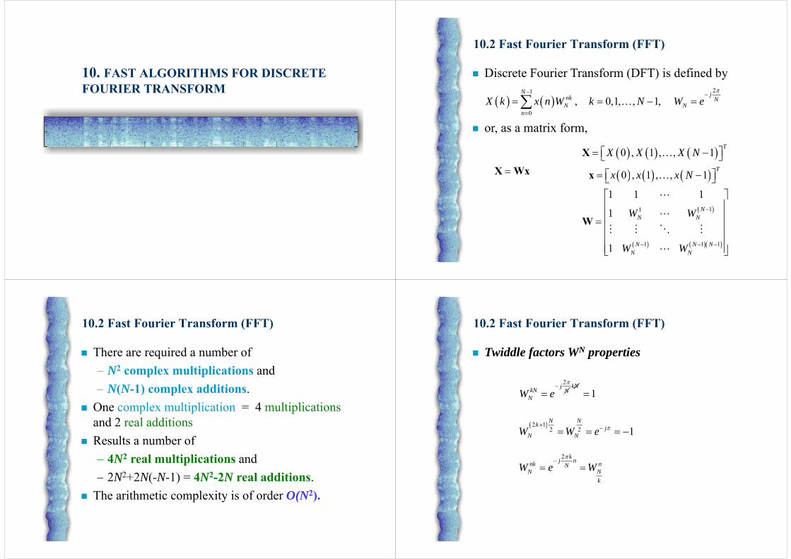
10. FAST ALGORITHMS FOR DISCRETE FOURIER TRANSFORM
10.2 Fast Fourier Transform (FFT)
Discrete Fourier Transform (DFT) is defined by
0. s ou e s o ( )
( ) y
21
, 0,1, , 1,N jnk N
N NX k x n W k N W e
or, as a matrix form,0n
X Wx
0 , 1 , , 1T
T
X X X N
X
X Wx 0 , 1 , , 1
1 1 1
Tx x x N
x
111 N
N NW W
W
1 1 11 N N N
N NW W
10.2 Fast Fourier Transform (FFT)
There are required a number of
0. s ou e s o ( )
q– N2 complex multiplications and
N(N 1) complex additions– N(N-1) complex additions. One complex multiplication = 4 multiplications
d 2 l dditiand 2 real additions Results a number of
– 4N2 real multiplications and – 2N2+2N(-N-1) = 4N2-2N real additions.2N 2N( N 1) 4N 2N real additions.
The arithmetic complexity is of order O(N2).
10.2 Fast Fourier Transform (FFT)
Twiddle factors WN properties
0. s ou e s o ( )
f p p
2j kNkN
1j
kN NNW e
N N 2 12 2 1N Nk j
N NW W e
2 kj nnk nNN N
k
W e W
k
10.2 Fast Fourier Transform (FFT)
There are algorithms that computes DFT with a
0. s ou e s o ( )
g psmaller number of operations.
An important case is where N=RM, R is called An important case is where N R , R is called radix.
There results FFT algorithms radix R There results FFT algorithms radix R. The index in the DFT formula can be expressed
i th f ll i l f lusing the following general formula:
1 1 2 2 modn K n K n N 1 1 2 2
3 1 4 2 modk K k K k N
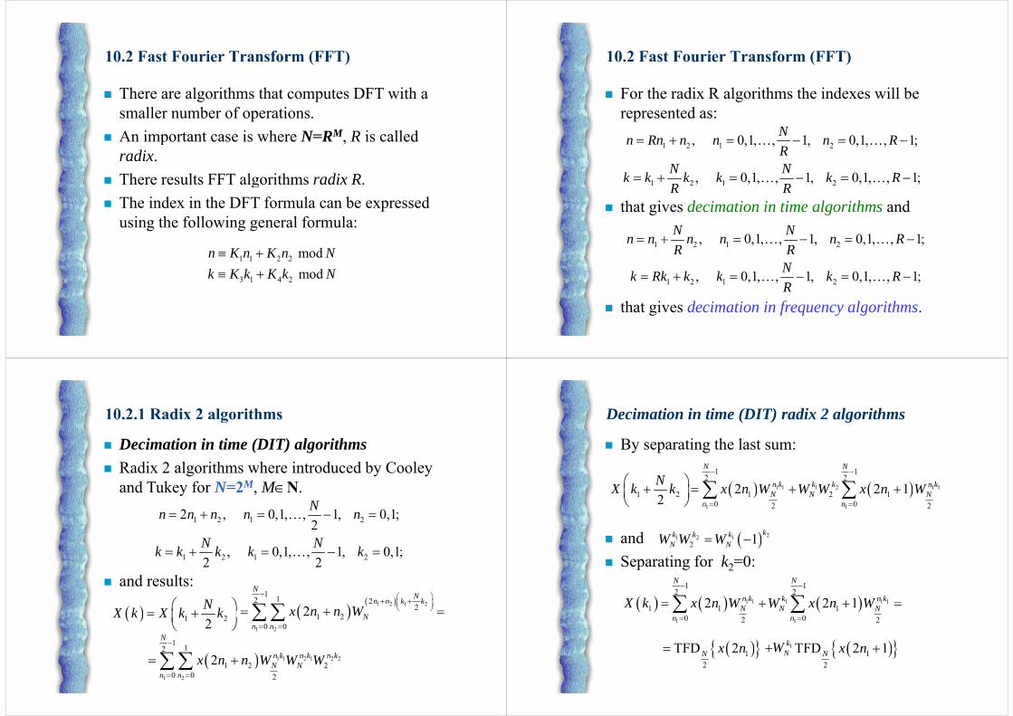
10.2 Fast Fourier Transform (FFT)
For the radix R algorithms the indexes will be
0. s ou e s o ( )
grepresented as:
0 1 1 0 1 1;Nn Rn n n n R 1 2 1 2, 0,1, , 1, 0,1, , 1;
0 1 1 0 1 1;
n Rn n n n RR
N Nk k k k k R
that gives decimation in time algorithms and1 2 1 2, 0,1, , 1, 0,1, , 1;k k k k k R
R R
1 2 1 2, 0,1, , 1, 0,1, , 1;N Nn n n n n RR R
1 2 1 2, 0,1, , 1, 0,1, , 1;Nk Rk k k k RR
that gives decimation in frequency algorithms.
10.2.1 Radix 2 algorithms
Decimation in time (DIT) algorithms
0. . d go s
Radix 2 algorithms where introduced by Cooley and Tukey for N=2M, MN.
1 2 1 22 , 0,1, , 1, 0,1;2Nn n n n n
d l1 2 1 2, 0,1, , 1, 0,1;
2 2N Nk k k k k
and results:
NX k X k k 1 2 1 2
1 12 22
1 22
NNn n k k
Nx n n W
1 22X k X k k
1 2
1 20 0
2 Nn n
x n n W
1 12
N
n k n k n k
1 1 2 1 2 2
1 2
1 2 20 0 2
2 n k n k n kN N
n nx n n W W W
Decimation in time (DIT) radix 2 algorithms
By separating the last sum:
eci atio i ti e ( ) adix algo it s
1 1 1 2 1 1
1 12 2
1 2 1 2 12 2 12
N N
n k k k n kN N N
NX k k x n W W W x n W
and
1 10 02 22 n n
21 2 1 1 kk k kW W W and Separating for k2=0:
21 2 12 1k k k
N NW W W
1 1 1 1 1
1 12 2
1 1 10 0
2 2 1
N N
n k k n kN N NX k x n W W x n W
1 10 02 2n n
1kNW 1TFD 2 1N x n 1TFD 2N x n N 1
2N 1
2N
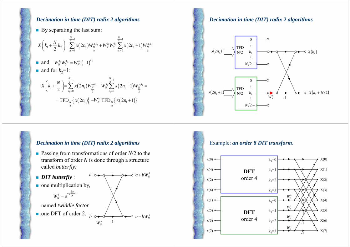
Decimation in time (DIT) radix 2 algorithms
By separating the last sum:
eci atio i ti e ( ) adix algo it s
1 1 1 2 1 1
1 12 2
1 2 1 2 12 2 12
N N
n k k k n kN N N
NX k k x n W W W x n W
and
1 10 02 22 n n
21 2 1 1 kk k kW W W and and for k2=1:
21 2 12 1k k k
N NW W W
1 1 1 1 1
1 12 2
1 1 12 2 12
N N
n k k n kN N N
NX k x n W W x n W
1 10 02 22 n n
1kNW 1TFD 2 1N x n 1TFD 2N x n N 1
2N 1
2N
Decimation in time (DIT) radix 2 algorithmseci atio i ti e ( ) adix algo it s
0
TFD
12nx 1k
TFD N/2 1kX
12 N
0
TFD
12 1 nx 1k
TFD N/2
1kNW
21 NkX -1
12 N
Decimation in time (DIT) radix 2 algorithmseci atio i ti e ( ) adix algo it s
Passing from transformations of order N/2 to the f f d N i d h htransform of order N is done through a structure
called butterfly:a k
Na bW DIT butterfly : one multiplication by one multiplication by,
2j kk NNW e
named twiddle factorDFT f d 2
N
-1 b k
Na bWk
NW
one DFT of order 2.
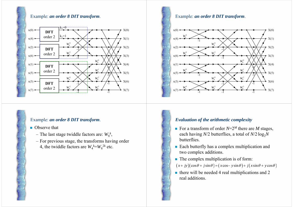
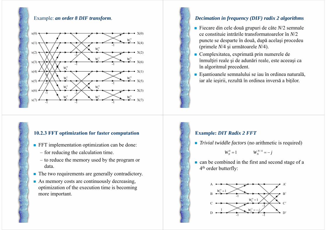
Example: an order 8 DIT transform.a p e: a o de 8 t a sfo .
(0) X(0)k 0x(0)
x(4) DFT
X(0)k1=0
X(1)k1=1
x(2)
DFTorder 4
1
X(2)k1=2
x(6)
( )0
8W( )
X(3)k1=3
x(1)
x(5) DFT-1
X(4)k1=01
8W1 X(5)k1=1
x(3)
DFTorder 4
-11
-1
28W
X(6)k1=23
x(7) -1
38W
X(7)k1=3
Example: an order 8 DIT transform.a p e: a o de 8 t a sfo .
(0) X(0)k1=0
x(0)
x(4)
X(0)
X(1)
DFTorder 2
1
k1=1
x(2) X(2)DFT -1
08W
2
08W
x(6)
( )
X(3)
( )
order 2-1
28W
-11
8W1
x(1)
x(5)
X(4)
X(5)
DFTorder 2
-1
08W
2-1
-12
8W
3
x(3) X(6)DFT
-1
28W
-1
38W
x(7) X(7)order 2
Example: an order 8 DIT transform.a p e: a o de 8 t a sfo .
(0) X(0)
1
08W
x(0)
x(4)
X(0)
X(1)-1
0-1
08W
2
x(2) X(2)
-1
08W
-1
28W
08W
x(6)
( )
X(3)
( )
1
08W
-11
8W1
x(1)
x(5)
X(4)
X(5)-1
0-1
08W
2-1
-12
8W
3
x(3) X(6)
-1
08W
-1
28W
-1
38W
x(7) X(7)
Example: an order 8 DIT transform. Observe that
h l iddl f k
a p e: a o de 8 t a sfo .
– The last stage twiddle factors are: W8k,
– For previous stage, the transforms having order 4, the twiddle factors are W4
k=W82k etc.
Evaluation of the arithmetic complexityvaluatio of t e a it etic co plexity
For a transform of order N=2M there are M stages, h h i N/2 b fli l f N/2 l Neach having N/2 butterflies, a total of N/2.log2N
butterflies. Each butterfly has a complex multiplication and
two complex additions. The complex multiplication is of form: cos sin cos sin sin cosx jy j x y j x y
there will be needed 4 real multiplications and 2real additions
cos sin cos sin sin cosx jy j x y j x y
real additions.
Evaluation of the arithmetic complexityvaluatio of t e a it etic co plexity
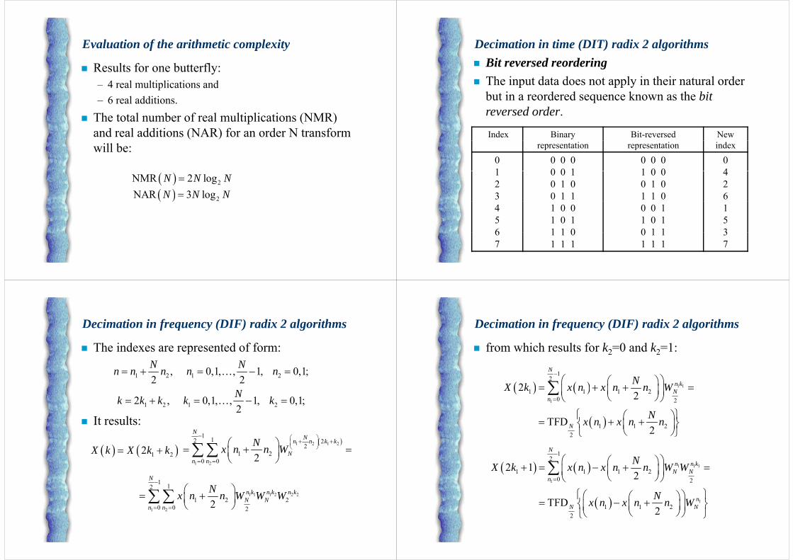
Results for one butterfly:– 4 real multiplications and– 6 real additions.
The total number of real multiplications (NMR) and real additions (NAR) for an order N transform will be:
2
2
NMR 2 logNAR 3 log
N N NN N N
Decimation in time (DIT) radix 2 algorithmseci atio i ti e ( ) adix algo it s Bit reversed reordering
Th i t d t d t l i th i t l d The input data does not apply in their natural order but in a reordered sequence known as the bit
d dreversed order.
Index Binary Bit-reversed New representation representation index
01
0 0 00 0 1
0 0 01 0 0
041
23
0 0 10 1 00 1 1
1 0 00 1 01 1 0
426
456
1 0 01 0 11 1 0
0 0 11 0 10 1 1
1536
71 1 01 1 1
0 1 11 1 1
37
Decimation in frequency (DIF) radix 2 algorithms
The indexes are represented of form:
eci atio i f eque cy ( ) adix algo it s
1 2 1 2, 0,1, , 1, 0,1;2 2N Nn n n n n
It results:1 2 1 22 , 0,1, , 1, 0,1;
2Nk k k k k
It results:
2X k X k k 1 2 1 2
1 12 22
NNn n k kNx n n W
1 22X k X k k
1 2
1 20 0 2 N
n nx n n W
1N
1 1 1 2 2 2
1 2
1 12
1 2 20 0 22
n k n k n kN N
n n
Nx n n W W W
Decimation in frequency (DIF) radix 2 algorithms
from which results for k2=0 and k2=1:
eci atio i f eque cy ( ) adix algo it s
1 1
12
1 1 1 22
N
n kNX k x n x n n W
1
1 1 1 20 2
22
TFD
Nn
X k x n x n n W
N
1 1 22
TFD2N x n x n n
N
1 1 1
1
12
1 1 1 20 2
2 12
N
n n kN N
n
NX k x n x n n W W
1
1
2
1 1 2TFD2
nN N
Nx n x n n W
2 2
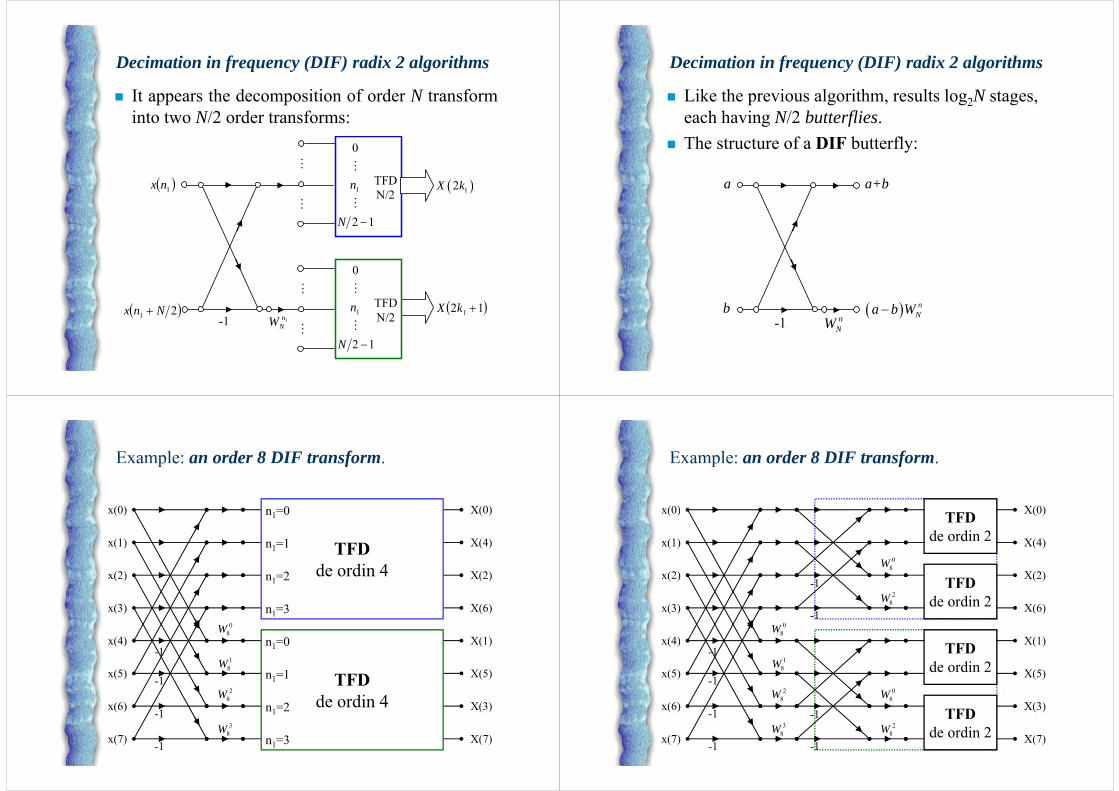
Decimation in frequency (DIF) radix 2 algorithms
It appears the decomposition of order N transformi N/2 d f
eci atio i f eque cy ( ) adix algo it s
into two N/2 order transforms: 0
1n
TFD N/2
1nx 12X k
12 N
N/2
0
-1 1n
21 Nnx
1nNW
TFD N/2
12 1 kX
12 N
N
Decimation in frequency (DIF) radix 2 algorithms
Like the previous algorithm, results log2N stages, h h i N/2 b fli
eci atio i f eque cy ( ) adix algo it s
each having N/2 butterflies. The structure of a DIF butterfly:
a a+b
-1 nNW
b nNa b W
NW
Example: an order 8 DIF transform.a p e: a o de 8 t a sfo .
X(0)(0) 0 X(0)
X(4)TFD
x(0) n1=0
x(1) n1=1
X(2)
TFDde ordin 4
1
x(2) n1=2
X(6)
( )0
8W( )
x(3) n1=3
X(1)
X(5)TFD-1
x(4) n1=01
8W1x(5) n1=1
X(3)
TFDde ordin 4
-1 12
8W
-1x(6) n1=23
X(7)3
8W-1x(7) n1=3
Example: an order 8 DIF transform.a p e: a o de 8 t a sfo .
(0) X(0)x(0)
x(1)
X(0)
X(4)
TFDde ordin 2
08W
2-1
x(2) X(2)TFD2
8W-1
08W
x(3)
( )
X(6)
( )
de ordin 2
18W
-1
1
x(4)
x(5)
X(1)
X(5)
TFDde ordin 2
08W
2-1
28W
3-1
-1
x(6) X(3)TFD2
8W-1
38W
-1x(7) X(7)de ordin 2
Example: an order 8 DIF transform.a p e: a o de 8 t a sfo .
(0) X(0)0
8W1
x(0)
x(1)
X(0)
X(4)0
8W
2 0
-1
-1x(2) X(2)
28W 0
8W-1-1
08W
x(3)
( )
X(6)
( )0
8W1
18W
-1
1
x(4)
x(5)
X(1)
X(5)0
8W
2 0
-1
-1
28W
3-1
-1
x(6) X(3)2
8W 08W
-1-1
38W
-1x(7) X(7)
Decimation in frequency (DIF) radix 2 algorithms
Fiecare din cele două grupuri de câte N/2 semnale i i i ă il f l î N/2
eci atio i f eque cy ( ) adix algo it s
ce constituie intrările transformatoarelor în N/2 puncte se desparte în două, după acelaşi procedeu ( i l N/4 i ă l N/4)(primele N/4 şi următoarele N/4).
Complexitatea, exprimată prin numerele de înmulţiri reale şi de adunări reale, este aceeaşi ca în algoritmul precedent.
Eşantioanele semnalului se iau în ordinea naturală, iar ale ieşirii, rezultă în ordinea inversă a biţilor. ş , ţ
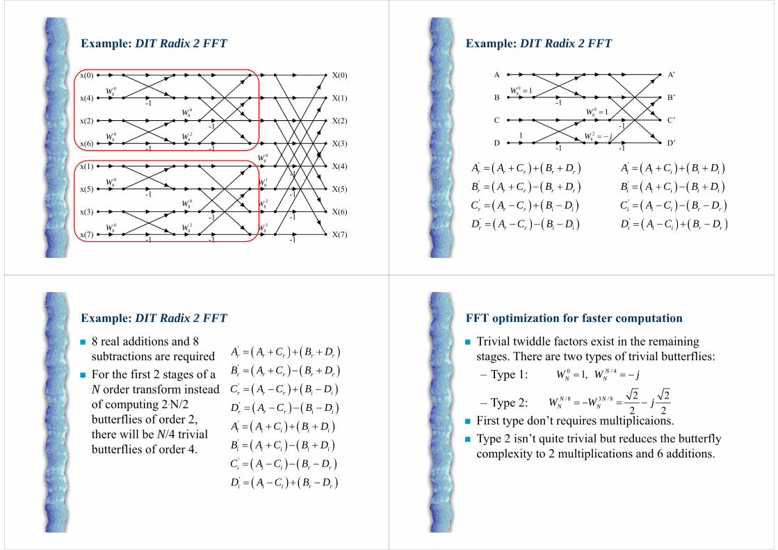
10.2.3 FFT optimization for faster computation
FFT implementation optimization can be done:
0. .3 op o o s e co pu o
p p– for reducing the calculation time.
to reduce the memory used by the program or– to reduce the memory used by the program or data.
Th t i t ll t di t The two requirements are generally contradictory. As memory costs are continuously decreasing,
optimization of the execution time is becoming more important.
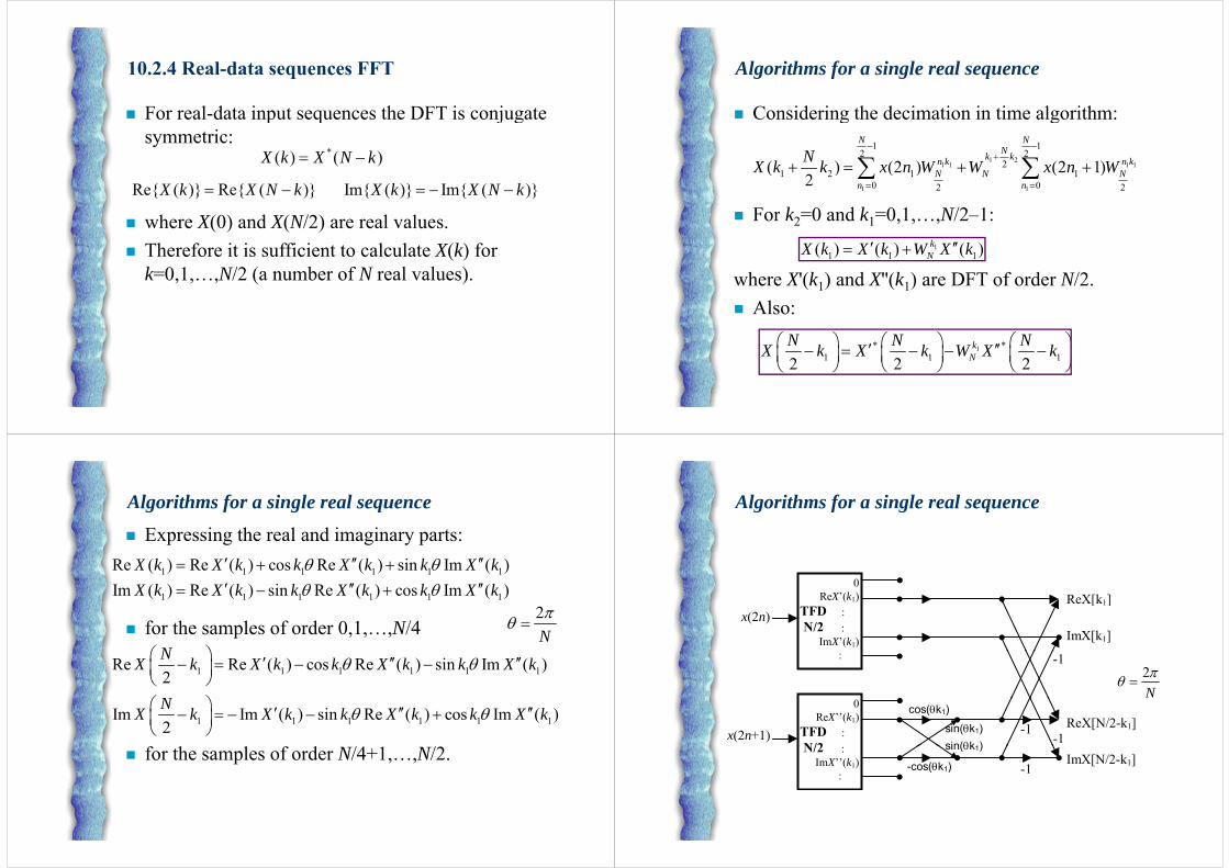
Example: DIT Radix 2 FFTp e: adix
Trivial twiddle factors (no arithmetic is required)0 1NW / 4N
NW j
can be combined in the first and second stage of a 4th order butterfly:
A A’
-1
08 1W
A
B
A
B’
-1
08 1W
2W j
C
1
C’
-1 -18W j
D1
D’
Example: DIT Radix 2 FFTp e: adix
x(0) X(0)
-1
08W
x(0)
x(4)
X(0)
X(1)
0W-1
08W
2W
x(2) X(2)
-18W
-18W
08W
x(6)
x(1)
X(3)
X(4)
-1
08W
-11
8W-1
x(1)
x(5)
X(4)
X(5)
0W-1
08W
2W-1
28W
3W
x(3) X(6)
-18W
-18W
-18W
x(7) X(7)
Example: DIT Radix 2 FFTp e: adix
A A’
-1
08 1W
B B’
-1
08 1W
28W j
C
1
C’
'A A C B D
-1 -18W j
D1
D’
'A A C B D '
r r r r r
r r r r r
A A C B D
B A C B D
'
i i i i i
i i i i i
A A C B D
B A C B D
'
'
r r r i i
r r r i i
C A C B D
D A C B D
'
'
i i i r r
i i i r r
C A C B D
D A C B D
r r r i i i i i r r
Example: DIT Radix 2 FFT
8 real additions and 8 b i i d
p e: adix
'A A C B D subtractions are required For the first 2 stages of a
'
r r r r r
r r r r r
A A C B D
B A C B D
N order transform instead of computing 2.N/2
'
'
r r r i i
r r r i i
C A C B D
D A C B D
butterflies of order 2, there will be N/4 trivial
'
'
r r r i i
i i i i iA A C B D
B A C B D
butterflies of order 4. '
i i i i i
i i i r r
B A C B D
C A C B D
'i i i r rD A C B D
FFT optimization for faster computationop o o s e co pu o
Trivial twiddle factors exist in the remaining Th f i i l b flistages. There are two types of trivial butterflies:
– Type 1: 0 / 41, NN NW W j
– Type 2: /8 3 /8 2 22 2
N NN NW W j
First type don’t requires multiplicaions. Type 2 isn’t quite trivial but reduces the butterfly
2 2
yp q ycomplexity to 2 multiplications and 6 additions.
10.2.4 Real-data sequences FFT
For real-data input sequences the DFT is conjugate
0. . e d seque ces
p q j gsymmetric:
*( ) ( )X k X N k
h X(0) d X(N/2) l lRe{ ( )} Re{ ( )}X k X N k Im{ ( )} Im{ ( )}X k X N k
where X(0) and X(N/2) are real values. Therefore it is sufficient to calculate X(k) for
k=0,1,…,N/2 (a number of N real values).
Algorithms for a single real sequence
Considering the decimation in time algorithm:
lgo it s fo a si gle eal seque ce
g g
1 21 1 1 1
1 12 2
2( ) (2 ) (2 1)
N NNk kn k n kNX k k x n W W x n W
For k2=0 and k1=0 1 N/2–1:1 1
1 2 1 10 02 2
( ) (2 ) (2 1)2 N N N
n nX k k x n W W x n W
For k2 0 and k1 0,1,…,N/2 1:1
1 1 1( ) ( ) ( )kNX k X k W X k
where X'(k1) and X''(k1) are DFT of order N/2. Also: Also:
1* *1 1 12 2 2
kN
N N NX k X k W X k
1 1 12 2 2N
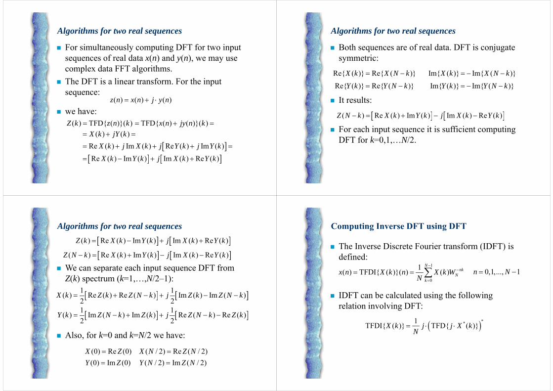
Algorithms for a single real sequence Expressing the real and imaginary parts:
lgo it s fo a si gle eal seque ce
1 1 1 1 1 1
1 1 1 1 1 1
Re ( ) Re ( ) cos Re ( ) sin Im ( )Im ( ) Re ( ) sin Re ( ) cos Im ( )
X k X k k X k k X kX k X k k X k k X k
for the samples of order 0,1,…,N/4N
2N
1 1 1 1 1 1Re Re ( ) cos Re ( ) sin Im ( )2NX k X k k X k k X k
N
1 1 1 1 1 1Im Im ( ) sin Re ( ) cos Im ( )2NX k X k k X k k X k
for the samples of order N/4+1,…,N/2.
Algorithms for a single real sequencelgo it s fo a si gle eal seque ce
0ReX’(k1) ReX[k1]
TFD : N/2 :
ImX’(k1)
x(2n)e [ 1]
ImX[k1] :
2N
-1
cos(k1)ReX[N/2-k1]-1x(2n+1)
0ReX’’(k1)
TFD :N/2
sin(k1)sin(k1)
-1ImX[N/2-k1]-1
N/2 :ImX’’(k1)
:-cos(k1)
sin(k1)
Algorithms for two real sequences
For simultaneously computing DFT for two input f l d ( ) d ( )
lgo it s fo two eal seque ces
sequences of real data x(n) and y(n), we may use complex data FFT algorithms.
The DFT is a linear transform. For the input sequence:
( ) ( ) ( )j we have:
( ) ( ) ( )z n x n j y n
( ) TFD{ ( )}( )Z k z n k( ) ( )X k jY k
TFD{ ( ) ( )}( )x n jy n k
Re ( ) Im ( ) Im ( ) Re ( )X k Y k j X k Y k
Re ( ) Im ( ) Re ( ) Im ( )X k j X k j Y k j Y k
( ) ( ) ( ) ( )j
Algorithms for two real sequences
Both sequences are of real data. DFT is conjugate i
lgo it s fo two eal seque ces
symmetric:Re{ ( )} Re{ ( )}X k X N k Im{ ( )} Im{ ( )}X k X N k
It lt
{ ( )} { ( )} { ( )} { ( )}Re{ ( )} Re{ ( )}Y k Y N k Im{ ( )} Im{ ( )}Y k Y N k
It results:
( ) Re ( ) Im ( ) Im ( ) Re ( )Z N k X k Y k j X k Y k
For each input sequence it is sufficient computing DFT for k=0 1 N/2
( ) ( ) ( ) ( ) ( )j
DFT for k 0,1,…N/2.
Algorithms for two real sequenceslgo it s fo two eal seque ces ( ) Re ( ) Im ( ) Im ( ) Re ( )Z k X k Y k j X k Y k
We can separate each input sequence DFT from ( ) Re ( ) Im ( ) Im ( ) Re ( )Z N k X k Y k j X k Y k
p p qZ(k) spectrum (k=1,…,N/2–1):
1 1( ) R ( ) R ( ) I ( ) I ( )X k Z k Z N k j Z k Z N k ( ) Re ( ) Re ( ) Im ( ) Im ( )2 2
X k Z k Z N k j Z k Z N k
1 1( ) Im ( ) Im ( ) Re ( ) Re ( )Y k Z N k Z k j Z N k Z k
Also for k=0 and k=N/2 we have:
( ) Im ( ) Im ( ) Re ( ) Re ( )2 2
Y k Z N k Z k j Z N k Z k
Also, for k 0 and k N/2 we have:
(0) Re (0) ( / 2) Re ( / 2)X Z X N Z N (0) Im (0) ( / 2) Im ( / 2)Y Z Y N Z N
Computing Inverse DFT using DFT
The Inverse Discrete Fourier transform (IDFT) is
Co pu g ve se us g
( )defined:
11( ) TFDI{ ( )}( ) ( )N
nkx n X k n X k W
0 1 1n N
IDFT b l l t d i th f ll i
0( ) TFDI{ ( )}( ) ( ) N
kx n X k n X k W
N
0,1,..., 1n N
IDFT can be calculated using the following relation involving DFT:
**1TFDI{ ( )} TFD{ ( )}X k j j X kN
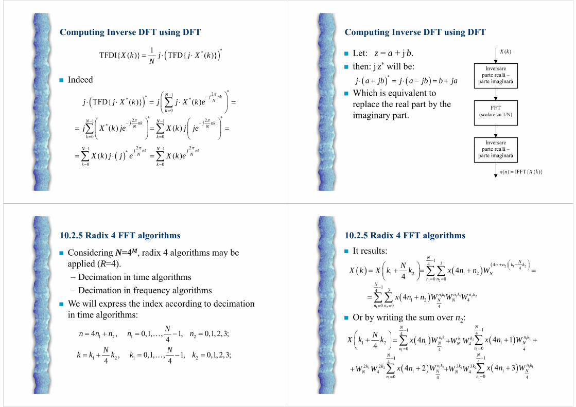
Computing Inverse DFT using DFTCo pu g ve se us g
**1TFDI{ ( )} TFD{ ( )}X k j j X k
Indeed
TFDI{ ( )} TFD{ ( )}X k j j X kN
Indeed
*21** *TFD{ ( )} ( )
N j nkNj j X k j j X k e
0
TFD{ ( )} ( )k
j j X k j j X k e
*21*
N j nk
*21N j nk *
0( )
j nkN
kj X k je
0( )
j nkN
kX k j je
2 2
21
*
0( )
N j nkN
kX k j j e
21
0( )
N j nkN
kX k e
Computing Inverse DFT using DFT
Let: z = a + j.b.
Co pu g ve se us g
( )X kj then: j.z* will be:
*j a jb j a jb b ja
Inversareparte reală –
i i ă
Which is equivalent tol th l t b th
j a jb j a jb b ja parte imaginară
replace the real part by theimaginary part.
FFT(scalare cu 1/N)
Inversareparte reală –
parte imaginară
( ) IFFT{ ( )}x n X k
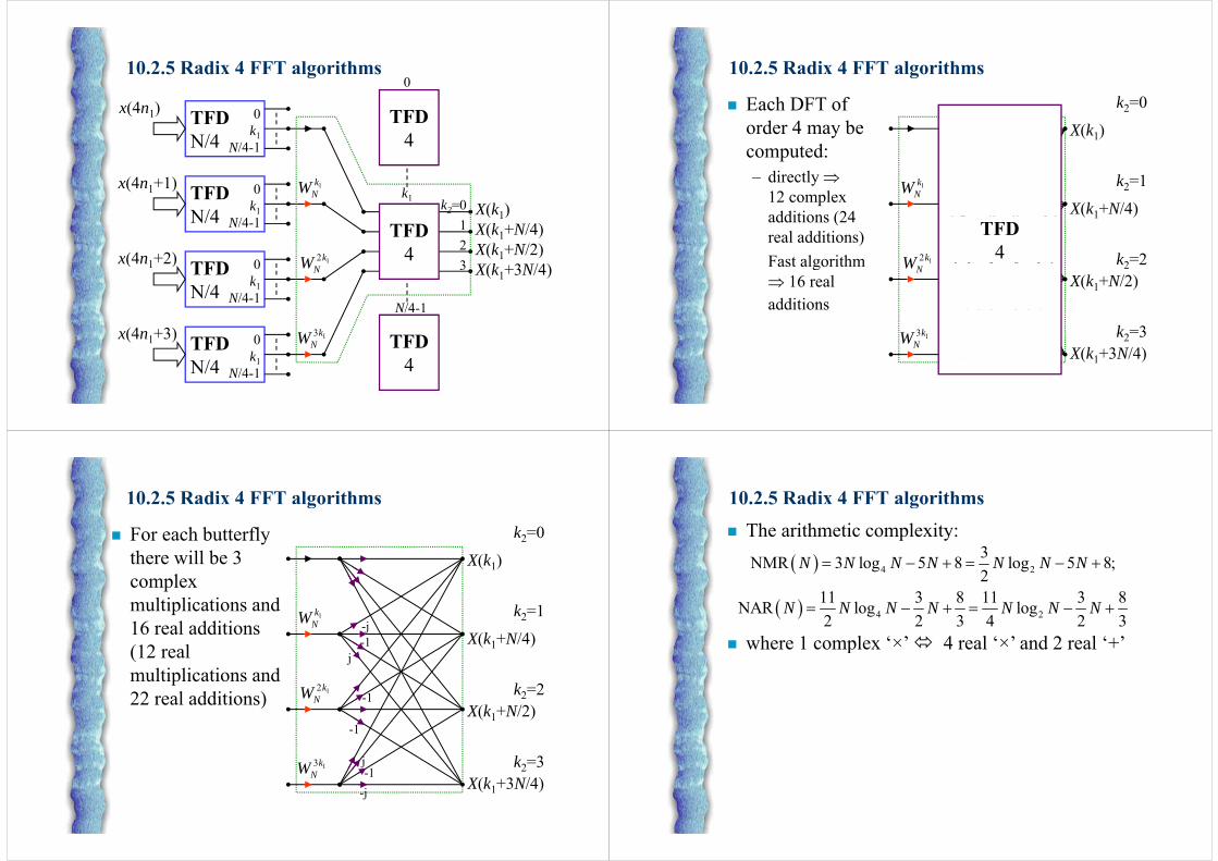
10.2.5 Radix 4 FFT algorithms
Considering N=4M, radix 4 algorithms may be li d (R 4)
0. .5 d go s
applied (R=4).– Decimation in time algorithms– Decimation in frequency algorithms
We will express the index according to decimation We will express the index according to decimation in time algorithms:
N1 2 1 24 , 0,1, , 1, 0,1,2,3;
4Nn n n n n
N N
1 2 1 2, 0,1, , 1, 0,1,2,3;4 4N Nk k k k k
10.2.5 Radix 4 FFT algorithms It results:
0. .5 d go s
1NN
1 24NX k X k k
1 2 1 2
1 2
1 34 44
1 20 0
4Nn n k k
Nn n
x n n W
N
1 1 2 1 2 2
1 34
1 2 40 0 4
4
N
n k n k n kN N
n nx n n W W W
Or by writing the sum over n2:1 20 0 4n n
N N
1 1
1
14
10 4
4
N
n kN
nx n W
1kNW 1 1
1
14
10 4
4 1
N
n kN
nx n W
1 24NX k k
2
4kW
1 0 4n
12kNW 13k
NW
1 4
1 1
14
14 2
N
n kNx n W
1 1
14
14 3
N
n kNx n W
224
kW 234
kWN N 1
10 4
Nn
1
10 4
Nn 4 4
10.2.5 Radix 4 FFT algorithms0. .5 d go s
x(4n1) TFD 0 TFD
0
TFDN/4 k1
N/4-1
TFD4
x(4n1+1) TFDN/4
0k1
1kNW
k2=0 X(k1)k1
N/4 N/4-1
x(4n1+2) TFD 0
TFD412kW
123
( 1)X(k1+N/4)X(k1+N/2)x(4n1 2) TFD
N/40
k1N/4-1
1NW 3 X(k1+3N/4)
N/4-1
x(4n1+3) TFD 0k
13kNW TFD
N/4 1
N/4 k1N/4-1 4
10.2.5 Radix 4 FFT algorithms0. .5 d go sk2=0 Each DFT of
d 4 b X(k1)order 4 may be computed:
1kNW
X(k1+N/4)-j
k2=1– directly 12 complex additions (24
12kW
( 1 )j
k2=2
additions (24 real additions)
– Fast algorithm
TFD41
NWX(k1+N/2)
-1
-1
k2 2Fast algorithm 16 real additions
13kNW
X(k1+3N/4)j-1
k2=3X(k1+3N/4)-j
10.2.5 Radix 4 FFT algorithms0. .5 d go sk2=0 For each butterfly
h ill b 3 X(k1)there will be 3 complex
l i li i d1k
NWX(k1+N/4)
-jk2=1multiplications and
16 real additions (12 l -1
12kW
( 1 )j
k2=2
(12 real multiplications and 22 l ddi i )
1
1NW
X(k1+N/2)-1
-1
k2 222 real additions)
13kNW
X(k1+3N/4)j-1
k2=3X(k1+3N/4)-j
10.2.5 Radix 4 FFT algorithms The arithmetic complexity:
0. .5 d go s
3 4 23NMR 3 log 5 8 log 5 8;2
11 3 8 11 3 8
N N N N N N N
where 1 complex ‘×’ 4 real ‘×’ and 2 real ‘+’
4 211 3 8 11 3 8NAR log log2 2 3 4 2 3
N N N N N N N
where 1 complex × 4 real × and 2 real +
![Algorithms Lecture 1: Discrete Probability [Sp’20] · 2020-04-07 · Algorithms Lecture 1: Discrete Probability [Sp’20] Moregenerally,acountablesetofeventsfAi ji 2Igisfullyormutuallyindependentifand](https://img.pdfslide.net/doc/110x75/5f8ded7df702d4365b6a0d5e/algorithms-lecture-1-discrete-probability-spa20-2020-04-07-algorithms-lecture.jpg)
![Algorithms Lecture 1: Discrete Probability [Sp’17]jeffe.cs.illinois.edu/teaching/algorithms/notes/01-random.pdf · Algorithms Lecture 1: Discrete Probability [Sp’17] The first](https://img.pdfslide.net/doc/110x75/5f8dedcb8dd33f5a0f7c51b1/algorithms-lecture-1-discrete-probability-spa17jeffecs-algorithms-lecture.jpg)