Gravity measurements below 10−9 g with atransportable absolute quantum gravimeterVincent Menoret1, Pierre Vermeulen1, Nicolas Le Moigne2, Sylvain Bonvalot3, PhilippeBouyer4, Arnaud Landragin5, and Bruno Desruelle1,*

1MUQUANS, Institut d’Optique d’Aquitaine, rue Francois Mitterrand, 33400, Talence, France2Geosciences Montpellier, CNRS, Universite Montpellier, UA, F–34095 Montpellier, France3GET, IRD, CNRS, CNES, Universite de Toulouse, F–31400 Toulouse, France4LP2N, Laboratoire de Photonique Numerique et Nanosciences, Institut d’Optique Graduate School, rue FrancoisMitterrand, 33400 Talence, France5LNE–SYRTE, Observatoire de Paris, Universite PSL, CNRS, Sorbonne Universite, 61 avenue de l’Observatoire,F–75014 Paris, France*bruno.desruelle@muquans.com

ABSTRACT

Gravimetry is a well-established technique for the determination of sub-surface mass distribution needed in several fields ofgeoscience, and various types of gravimeters have been developed over the last 50 years. Among them, quantum gravimetersbased on atom interferometry have shown top-level performance in terms of sensitivity, long-term stability and accuracy.Nevertheless, they have remained confined to laboratories due to their complex operation and high sensitivity to the externalenvironment. Here we report on a novel, transportable, quantum gravimeter that can be operated under real world conditionsby non-specialists, and measure the absolute gravitational acceleration continuously with a long-term stability below 10 nm.s−2

(1 µGal). It features several technological innovations that allow for high-precision gravity measurements, while keeping theinstrument light and small enough for field measurements. The instrument was characterized in detail and its stability wasevaluated during a month-long measurement campaign.

IntroductionOver the past few decades, gravimetry has proven a powerful tool for geoscience. Its potential in many different fields has beendiscussed in detail1. The value of gravity at the Earth’s surface is directly related to sub-surface mass distribution, and theanalysis of both the temporal and spatial variations of the gravitational field has allowed for the characterization of severalgeophysical phenomena – including ice mass changes2, 3, the monitoring of volcanoes4 and ground water resources5, 6, thestudy of subsidence in low-lying areas7, the monitoring of geothermal reservoirs8 and the detection of underground cavities9.

Earth’s gravitational acceleration g varies roughly between 9.78 m.s−2 and 9.83 m.s−2 over the whole Earth. The dailyfluctuation, induced by the deformation of the planet by tides, is about 10−7 g. The variations of g investigated in geoscience areusually at a smaller level and the level of relative precision required for an operational instrument is of the order of one part perbillion, or 10 nm.s−2 (1 µGal). Several technological solutions have been developed to reach this demanding requirement, andthe instruments used over the past 50 years were reviewed by Van Camp et al1. Absolute gravimeters yield an accurate value ofg and are necessary to calibrate relative instruments and measure their drift. They are usually based on the measurement of thedistance traveled by a free-falling corner-cube reflector in a vacuum chamber by laser interferometry10. While such absolutegravimeters can nowadays be operated in the field, the technology still makes it difficult to reach both the best operability andsensitivity. In particular, these instruments have moving mechanical parts that make them unsuitable for long-term continuousmeasurements.

Absolute measurements at the level of 10 nm.s−2 have also been demonstrated with gravimeters based on atom interferome-try11–13, which rely on the wave nature of matter postulated by quantum mechanics. Similar to classical absolute gravimeters,they measure the acceleration of free-fall test masses (in this case cold atoms) compared to the local ground reference frame.Atomic gravimeters have already demonstrated top-level performance in terms of sensitivity, long-term stability and accuracyin international comparisons14–20, and several demonstrations have shown promise for in-field and onboard applications16, 21–23.However, these instruments were not practically suited for geophysical surveys because of their limited transportability andhigh complexity.

Here, we report on both operability and sensitivity at the level of 10 nm.s−2 with an atomic gravimeter. Our novel Absolute

arX

iv:1

809.

0490

8v1

[ph

ysic

s.at

om-p

h] 1

3 Se

p 20

18

Quantum Gravimeter (AQG) includes conceptual and technological developments that made it possible to reach compactness,transportability, low maintenance and non-expert operation, both for continuous observatory measurements and gravity mapping.These developments include a hollow pyramid reflector24, 25 and a compact telecom based laser system. The resulting sensormeasures gravity at a 2 Hz repetition rate with a sensitivity of 500 nm.s−2.Hz−1/2 and a long term stability below 10 nm.s−2

with a short installation and warm-up time. Combined, these features represent a significant technological step forward, andhave enabled the first long-term measurement campaign with a quantum gravimeter in a geophysical observatory, whichcomprised several weeks of continuous gravity measurements on the Larzac plateau in France.

The Absolute Quantum GravimeterMeasurement principleThe AQG measurement sequence is based on matter-wave interferometry with Rubidium atoms using two-photon stimulatedRaman transitions11. This type of sequence has been extensively studied and used for precision measurements12, 14–16. Here, wegive a brief description of the measurement principle; the step-by-step procedure can be found in the Supplementary Methods.

The sequence consists of three counterpropagating Raman pulses of duration 10, 20 and 10 µs in a π/2− π − π/2configuration. Between these pulses, the the atoms are in near-perfect free fall for an interrogation time of T = 60 ms. Theoutput ports of the interferometer are labeled by the internal states |52S1/2,F = 1,mF = 0〉 and |52S1/2,F = 2,mF = 0〉 of theatom27. Fluorescence detection is used to count the number of atoms in each level and measure the interferometric phaseshift. For cooling, Raman and fluorescence detection, the lasers are tuned close to the D2 line of 87Rb, with a wavelengthλ ≈ 780 nm. The proportion of atoms in the F = 2 state is given by

P = 0.5× (1−C cosΦ) (1)

where C is the contrast of the fringes and Φ the interferometric phase shift. The contrast of the fringes is lower than 1, mainlybecause of velocity selection effects during the Raman pulses28. The phase shift Φ is given by

Φ = (keffg−2πα)T 2, (2)

where keff = 4π/λ ≈ 16×106 m−1 is the effective wavevector of the two-photon transition and α ≈ 25 MHz.s−1 is a frequencychirp applied to the Raman lasers to compensate the Doppler effect. We operate the instrument around the null phase shiftby servo-locking the frequency chirp α on the detection ratio P so as to constantly maintain keffg−2πα = 0 and stay on thecentral fringe of the interferometer29. From there we derive

g = 2πα

keff. (3)

The sensitivity of the instrument is limited both by the signal-to-noise ratio of the detection and by the contrast. A contrastC of 40% and a detection signal-to-noise ratio of 150 correspond to an effective signal-to-noise ratio (SNR) of 0.4×150 = 60.At mid-fringe, the sensitivity is given by

δgg

=1

keffgT 2SNR. (4)

With the previous parameters, δg/g≈ 3×10−8. This constitutes the single-shot sensitivity floor of the instrument, but thisquantity can be deteriorated by other factors, such as laser phase noise or vibrations15. However, since the instrument’srepetition rate is on the order of 2 Hz, the performance is improved by averaging over time to reach a long-term relative stabilityclose to 1×10−9.

Instrument descriptionThe AQG is made of two sub-units, the sensor head and the control system (fig. 1). The sensor head houses the vacuumchamber where the measurement of gravity is performed. It can easily be set up at the measurement location, and is separatedfrom the laser system and control electronics by a 5 m set of cables, which includes an optical fiber. The instrument can beinstalled in less than 20 min and is ready to measure after 1 h of warm-up time. The only adjustment to be performed by theoperator during the installation process is setting the verticality of the sensor head. The angle is measured by two tiltmeters andthe software indicates how the leveling tripod screws should be turned. Using this procedure, an operator can reach a verticalityerror of approximately 100 µrad. When not in use, the gravimeter can be completely powered off for several weeks with nosignificant impact on its vacuum level or warm-up time.

2/13

Up to 5 m

70

cm

Sensor head

Laser system andcontrol electronics

DetectionF=2F=1

π/2

π/2

π Atominterferometerpulses

Cooler / RepumperorRaman 1 / Raman 2

Pyramidreflector

MOT coils

Accelerometer,barometer andtiltmeters

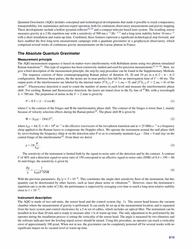
Figure 1. Left: picture of the first Absolute Quantum Gravimeter (AQG-A01). The system can be setup at a measurementlocation in less than 20 min, warm-up time is of the order of 1 h. The sensor head weighs approximately 30 kg. It is mountedon an adjustable tripod with precision leveling titanium-tipped feet that can be adapted to various terrains. The measurementheight is 55 cm. Right: sketch of the sensor head and measurement principle24. Approximately 107 atoms are loaded in amagneto-optical trap (MOT) inside the pyramid and cooled down to 2 µK. The π/2−π−π/2 atom interferometry sequenceis performed once the atoms are in free-fall. At the end of the sequence, we collect fluorescence on a set of photodiodes andcompute the proportion of atoms in each output port of the interferometer, labeled by their internal state. A high-precisionaccelerometer is attached to the top of the vacuum chamber, as close as possible to the pyramidal reflector. Its signal is used toapply a real-time correction to the laser phase, in order to reject seismic noise. Two tiltmeters and a barometer are also attachedto the sensor to ensure high accuracy and long-term stability of the gravity measurement.

Using a pyramidal reflector and a single-beam geometry, we load 107 87Rb atoms in a magneto-optical trap (MOT) in250 ms and cool them down below 2 µK in an optical molasses. We then select the atoms in the |F = 1,mF = 0〉 state by usinga microwave selection. After approximately 30 ms (4.4 mm) of free-fall, the atoms exit the pyramidal reflector and we applythe π/2−π−π/2 sequence of Raman laser pulses with the parameters described above (τ = 10 µs, T = 60 ms, C = 40%).The interferometer pulses are delivered by the same laser as the one used for cooling and detection, the compact configurationwith the pyramidal reflector allows the use of a single beam as demonstrated by Bodart et al24. At the bottom of the chamber(150 mm below the position of the trap), we measure the proportion of atoms in each output port of the interferometer with adetection signal-to-noise ratio of 150. We lock the frequency chirp to the atomic signal in order to stay on the central fringe ofthe interferometer and derive g from the values of α and keff. To measure gravity at the 10−9 level, both of these parametersmust be known with an uncertainty lower than 1 part in 109. We also periodically reverse the orientation of the effective Ramanwavevector to reject the systematic effects that do not depend on the sign of keff

29.

Laser systemThe stability and performance of the laser system and control electronics are crucial for both the quality of the gravitymeasurement and the way the instrument is operated. In particular, the spectral properties of the laser will have an influence onthe signal-to-noise ratio and long-term stability of the measurement. Its size, weight, robustness and ease of use determine thelevel of transportability and convenience for a daily operation of the gravimeter.

Our laser system complies with these constraints by using a frequency-doubled telecom solution30, 31. Lasers operatingin the telecom C-band around 1560 nm are amplified and converted to 780 nm in nonlinear crystals. The laser system iscompletely fibered, making it insensitive to misalignments and vibrations. Our architecture is based on a fixed-frequencyreference laser, and two independent tunable slave lasers.

A master reference laser diode, emitting at 1560 nm, is frequency-doubled in a periodically-poled lithium niobate (PPLN)

3/13

waveguide crystal and frequency locked to the F = 3 to F = 4 crossover transition of 85Rb using saturated absorptionspectroscopy. Two slave lasers, used for both cooling and Raman excitation are frequency offset-locked to the master laser.Their frequency can be tuned up to 1 GHz in 200 µs. The first slave laser addresses the |52S1/2,F = 1〉 level (repumping andRaman 1) and the second one is near-resonant with the |52S1/2,F = 2〉 level (cooling and Raman 2). At the beginning of theRaman interferometer, the lasers are detuned by approximately 700 MHz and the frequency lock loop of the cooling and Raman2 laser is switched to a phase lock loop on the Raman 1 laser, which remains frequency-locked to the reference laser. The phasedifference between the two Raman lasers has a direct influence on the phase shift Φ of the atom interferometer11, 32. The phaselock loop is therefore necessary to ensure that that the level of residual phase noise does not deteriorate the sensitivity of thegravimeter.

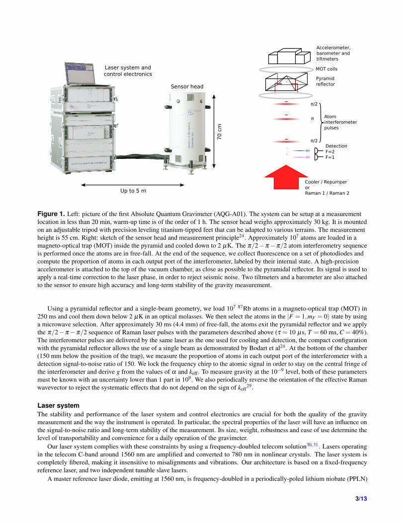
To amplify the lasers, we have developed custom Erbium-Doped Fiber Amplifiers (EDFA) that deliver an output ofapproximately 500 mW. The power efficiency of these EDFAs has been optimized to around 10 % and their AmplifiedSpontaneous Emission kept to a low level, with a noise figure below 6 dB. After amplification, we use waveguide PPLNcrystals to convert light from 1560 to 780 nm. For each slave laser, we obtain a power of approximately 250 mW at 780 nm,corresponding to a conversion efficiency of the order of 50%. The two lasers are then combined in the same fiber using apolarization multiplexer and injected in a custom-made fibered AOM that sets the total output power and drives the Ramanpulses. Light is finally sent in a polarization-maintaining fiber to the sensor head. At the fiber output, the power in eachwavelength is approximately 150 mW and polarization extinction ratio is higher than 20 dB. We have characterized the linewidthof the laser by recording a beatnote between the gravimeter and a similar independent laser system (see Methods). We find alorentzian linewidth of 12 kHz (Fig. 2), which is low enough not to limit atomic cooling and detection.

Figure 2. Laser linewidth (left) and long-term frequency stability measurements (right). We make a beatnote between thelaser of the gravimeter and a similar independent laser. A Lorentzian fit of the tails of the beatnote gives a linewidth of less than12 kHz for each laser. By recording the frequency of the beatnote over time on a frequency counter, we can estimate thelong-term frequency stability of the lasers. Here, the standard deviation over four days is 27 kHz, and no significant drift isvisible on the measurement.

Sensor headAs the sensor head is intended to be installed in the field, its overall weight, compactness and ease of manipulation areessential. In this respect, we use a hollow pyramidal reflector inspired by the one described by Bodart et al.24 to implement allthe functions required by the measurement sequence with a single laser beam, leading to a significant reduction in volume,complexity and risk of misalignment (Fig. 1).

The optical characteristics of the reflector are critical for the performance of the instrument, both in terms of polarizationand wavefront aberrations33. The inner faces of the reflector are coated for maximum reflection at 45◦ and for equal phase-shiftbetween the two orthogonal polarizations. Therefore, reflections of the single circularly-polarized beam onto the four innerfaces of the pyramid create the required polarization configuration for the magneto-optical trap and molasses inside thepyramid. In addition, below the pyramid the retro-reflected laser beam can drive counter-propagating Raman transitions in aσ+/σ+ or σ−/σ− configuration to create the matter-wave interferometer. This polarization configuration is also suitable forfluorescence detection. The wavefront of the retroreflected beam has been characterized in detail and its quality is better than

4/13

λ/80 (peak-to-valley, 780 nm) in the center region used for the atom interferometer.The vacuum chamber is protected from external magnetic fields by two layers of mu-metal shields. A high-performance

accelerometer is attached to the top of the vacuum chamber in order to implement an active compensation of vibrations and tomake the instrument robust against seismic noise without the need of an isolation device34, 35. Two tiltmeters are also includedin the sensor head to ensure the AQG is perfectly vertical, and are used to measure any long-term angular drift. Finally, abarometer is used to monitor the atmospheric pressure and correct its effect on the measurement. Because gravity gradients areof the order of 3000 nm.s−2.m−1, it is important to know the effective measurement height of the instrument. On the AQG thisis, on average, 55 cm above ground level. The measurement height above the leveling tripod is precisely known by design to be48.8 cm and the height of the tripod above the ground can be measured with a precision of 1 mm during the installation of theinstrument.

Instrument controlField conditions require the instrument to be stable and simple to operate. The control software of the AQG takes theseconstraints into account. All the operations required to start the gravimeter are automated: the software automatically locks thelasers to a predefined setpoint, turns on the EDFAs and starts the measurement sequence. Monitoring of several parameters,such as optical powers and lock stability, has been implemented and corrections are automatically applied when necessary. Wehave demonstrated that the laser and electronics system can run continuously for several months without breaking out of lock.At the start of the measurement sequence, the software checks additional parameters such as atom number and laser intensity,and selects the central fringe of the interferometer that gives the initial value of g required to initiate the gravity measurement(see Supplementary Methods). By monitoring critical parameters over time, the software is able to detect if the instrument isunstable or requires attention.

In addition to these features, the software also calculates tilts, atmospheric pressure, vertical gravity gradients, polar motionand quartz oscillator frequency drifts. Earth tide and ocean loading corrections are also implemented, by calling a TSoftroutine36. Several display options are available to check the quality of the measurement in real time. Remote access to thegravimeter is possible using an internet connection, both to retrieve data and to control the instrument.

Results

Scale factor verificationThe value of gravity is computed from the effective wavevector and the frequency chirp as indicated in equation (3). Bothof these parameters contribute to the scale factor of the gravimeter and to the final precision of the measurement. We havemeasured their mean values and long-term stability at the level of a few 10−10.

The frequency chirp α is generated using a compact microwave synthesizer with a quartz reference oscillator. The absolutevalue and long-term stability of the output frequency can be calibrated using the gravimeter itself, by operating it as an atomicclock. At given time intervals, the gravity measurement is paused for approximately 30 s and the instrument switches froma Raman to a Ramsey π/2−π/2 sequence where microwave pulses are driven by the microwave synthesizer. The resultingsignal allows us to measure the frequency of the oscillator with an uncertainty lower than 1 part in 1010. We correct the value ofα and g accordingly, making the residual contribution lower than 1 nm.s−2.

To ensure an absolute calibration of the laser frequencies, the system is referenced to a Rubidium optical transition at afrequency f = c/λ ≈ 384 THz using saturated absorption spectroscopy. Therefore, measuring gravity with a long-term relativestability better than 10−9 requires the laser frequencies to be known with an uncertainty below 384 kHz. To characterizelaser frequency stability, we use the same setup as for the linewidth measurement (see Methods). We find that the long-termfrequency stability is lower than 30 kHz rms over several days (Fig. 2), and that the effective wavector is both accurate andstable enough for the operation of the gravimeter.

Mitigation of external effectsIn order to avoid a degradation of the instrument’s sensitivity by seismic noise, we have implemented an active compensation ofvibrations, originally described by Merlet et al.34 and Lautier et al.35. A high-performance classical accelerometer is attachedto the top of the vacuum flange that supports the pyramidal reflector. This mechanical structure is very rigid by design so thatthe recorded signal is not distorted by resonances or deflections. The signal is filtered, digitized and weighed by the accelerationtransfer function of the atom interferometer in real time (see Methods). Just before the last pulse of the interferometer a phasecorrection corresponding to the integrated acceleration noise is applied to the Raman lasers. The value of phase correction canbe stored so that no information is lost in the process. In our laboratory in Talence (France), there is a high level of vibrationnoise. The integrated seismic noise typically corresponds to phase shifts of 2.3 rad rms (20 rad peak-to-peak), meaning theinterference fringes are completely blurred. Using this real-time compensation, we recover the fringes and keep the residual

5/13

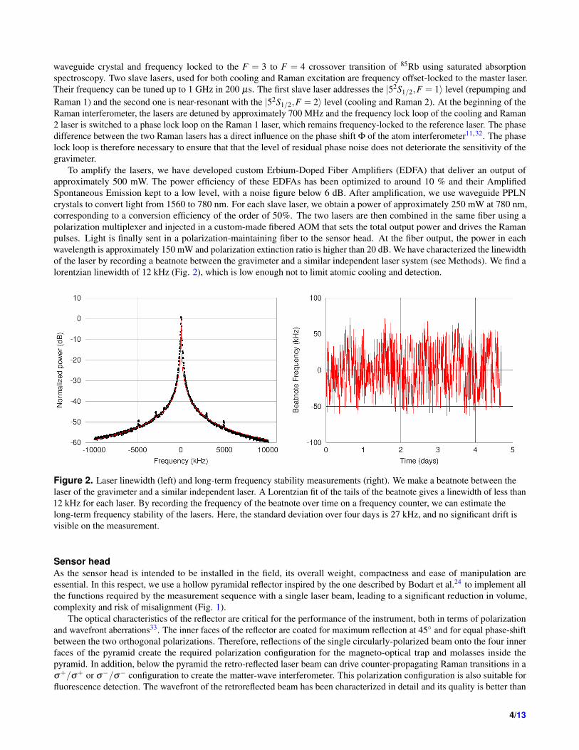
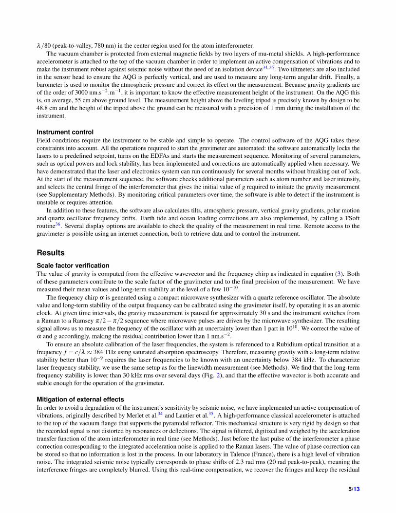
acceleration noise to a level of approximately 36 mrad rms (250 mrad pk-pk), corresponding to a rejection factor higher than 60(Fig. 3). This techniques allows the AQG to perform sub 10−9g measurements even in these noisy conditions.

Figure 3. Active compensation of vibrations. Left: atom interferometer fringes scanned by varying the Raman chirp α . Bluecrosses: without active compensation. Red line: with active compensation. Error bars correspond to the standard deviation over20 measurements. Right: the gravimeter is operated close to mid-fringe and we measure the ratio of atoms in each internal state.During the first 1000 cycles, the compensation is turned off. Phase noise due to vibrations is 2.3 rad rms, and the interferencesignal is washed out over several fringes. During the last 1000 cycles, active compensation is turned on and the vibration phasenoise is greatly reduced to 36 mrad rms, allowing the interferometer to remain close to mid-fringe.

The two high-precision tiltmeters are used to measure the tilts of the instrument in the horizontal plane and derive thevertical angle. An initial absolute calibration of the tiltmeters has been performed with the gravimeter itself (see Methods).This calibration ensures that the angle is known with an uncertainty better than 10 µrad, which keeps the error on the value ofg below 10 nm.s−2. The tiltmeters are first used during the installation phase to make sure the gravimeter is vertical. Whenthe instrument is running, tilt values are continuously monitored and the corresponding correction is applied to g so as tocorrect any long-term deviation from verticality and maintain the stability of the AQG below 10 nm.s−2. Similarly, we use thebarometer to measure atmospheric pressure variations with an accuracy better than 1 hPa. Since pressure admittance37 is of theorder of −3 nm.s−2.hPa−1, this is sufficient to ensure that the residual effect due to the barometer is lower than 10 nm.s−2.

Sensitivity and stability measurementsWe have operated the AQG-A01 in several locations to validate its operability and transportability. In this section we discussmeasurements obtained in two locations with different levels of vibration noise. The first one is the laboratory of Muquans,located in Talence (suburb of Bordeaux, France). This site features a high level of microseismic noise due to its proximity tothe ocean and its location on the second floor of an inner-city building constructed on sediments. The second site is the Larzacobservatory in the south of France6, 38. This site is dedicated to hydrology studies and local gravity has been measured there byabsolute and relative gravimeters on a regular basis since 2006. The Larzac observatory has a very low level of high-frequencyvibration noise (i.e. above 1 Hz) compared to Talence. A comparison of noise levels measured with the accelerometer ofthe AQG in both locations is shown in the Methods section. In both cases, gravity data are acquired by the AQG at a rate ofapproximately 2 Hz. These data are then averaged to improve statistical uncertainty, and corrected for tilt variations, drifts ofthe microwave oscillator, and atmospheric pressure using the admittance. Gravity data are also corrected by a synthetic tide,with parameters determined by analyzing a 9-month recording by a CG5 relative gravimeter in Talence, and a 3-year recordingperformed by a superconducting gravimeter in Larzac.

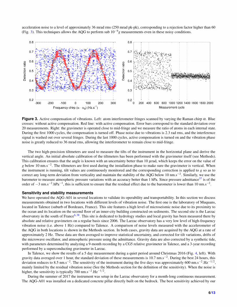
In Talence, we show the results of a 5 day measurement during a quiet period around Christmas 2016 (Fig. 4, left). Withgravity data averaged over 1 hour, the standard deviation of these measurements is 10.7 nm.s−2. During the best 24 hours, thisdeviation reduces to 8.5 nm.s−2. The sensitivity of the instrument during the five days was approximately 600 nm.s−2.Hz−1/2,mainly limited by the residual vibration noise (See the Methods section for the definition of the sensitivity). When the noise ishigher, the sensitivity is typically 700 nm.s−2.Hz−1/2.

During the summer of 2017 the instrument was setup in the Larzac observatory for a month-long continuous measurement.The AQG-A01 was installed on a dedicated concrete pillar directly built on the bedrock. The best sensitivity achieved by our

6/13

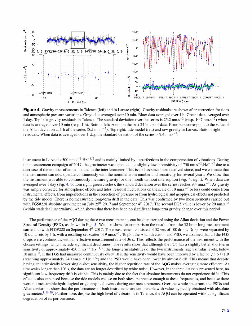
Figure 4. Gravity measurements in Talence (left) and in Larzac (right). Gravity residuals are shown after correction for tidesand atmospheric pressure variations. Grey: data averaged over 10 min. Blue: data averaged over 1 h. Green: data averaged over1 day. Top left: gravity residuals in Talence. The standard deviation over the series is 25.2 nm.s−2 (resp. 10.7 nm.s−2) whendata is averaged over 10 min (resp. 1 h). Bottom left: zoom on the best 24 hours of data. Error bars correspond to the value ofthe Allan deviation at 1 h of the series (8.5 nm.s−2). Top right: tide model (red) and raw gravity in Larzac. Bottom right:residuals. When data is averaged over 1 day, the standard deviation of the series is 9.4 nm.s−2.

instrument in Larzac is 500 nm.s−2.Hz−1/2 and is mainly limited by imperfections in the compensation of vibrations. Duringthe measurement campaign of 2017, the gravimeter was operated at a slightly lower sensitivity of 750 nm.s−2.Hz−1/2 due to adecrease of the number of atoms loaded in the interferometer. This issue has since been resolved since, and we estimate thatthe instrument can now operate continuously with the nominal atom number and sensitivity for several years. We show thatthe instrument was able to continuously measure gravity for one month without interruption (Fig. 4, right). When data areaveraged over 1 day (Fig. 4, bottom right, green circles), the standard deviation over the series reaches 9.4 nm.s−2. As gravitywas simply corrected for atmospheric effects and tides, residual fluctuations on the scale of 10 nm.s−2 or less could come frominstrumental effects, from imperfections in the correction of pressure or from hydrological and geophysical effects not predictedby the tide model. There is no measurable long-term drift in the data. This was confirmed by two measurements carried outwith FG5#228 absolute gravimeter on July 25th 2017 and September 4th 2017. The second FG5 value is lower by 20 nm.s−2

(within statistical uncertainty), which shows that there has been no significant long-term gravity change over this period.

The performance of the AQG during these two measurements can be characterized using the Allan deviation and the PowerSpectral Density (PSD), as shown in Fig. 5. We also show for comparison the results from the 32 hour long measurementcarried out with FG5#228 on September 4th 2017. The measurement consisted of 32 sets of 100 drops. Drops were separated by10 s and sets by 1 h, with a resulting set-scatter of 9 nm.s−2. To plot the Allan deviation and PSD, we assumed that all the FG5drops were continuous, with an effective measurement rate of 36 s. This reflects the performance of the instrument with thechosen settings, which include significant dead times. The results show that although the FG5 has a slightly better short-termsensitivity of approximately 450 nm.s−2.Hz−1/2, the long-term stabilities of the two instruments reach similar levels, below10 nm.s−2. If the FG5 had measured continuously every 10 s, the sensitivity would have been improved by a factor

√3.6≈ 1.9

(reaching approximately 240 nm.s−2.Hz−1/2) and the PSD would have been lower by almost 6 dB. This means that despitehaving an intrinsically lower single-shot sensitivity, the higher repetition rate of the AQG makes averaging more efficient. Attimescales longer than 104 s, the data are no longer described by white noise. However, in the three datasets presented here, nosignificant low-frequency drift is visible. This is mainly due to the fact that absolute instruments do not experience drifts. Thiseffect is also enhanced because the tide models we use on both sites are precise enough at these frequencies, and because therewere no measurable hydrological or geophysical events during our measurements. Over the whole spectrum, the PSDs andAllan deviations show that the performances of both instruments are comparable with values typically obtained with absolutegravimeters1, 16, 39. Furthermore, despite the high level of vibrations in Talence, the AQG can be operated without significantdegradation of its performance.

7/13

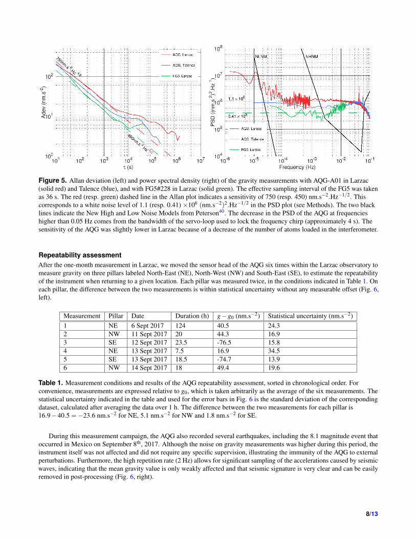
Figure 5. Allan deviation (left) and power spectral density (right) of the gravity measurements with AQG-A01 in Larzac(solid red) and Talence (blue), and with FG5#228 in Larzac (solid green). The effective sampling interval of the FG5 was takenas 36 s. The red (resp. green) dashed line in the Allan plot indicates a sensitivity of 750 (resp. 450) nm.s−2.Hz−1/2. Thiscorresponds to a white noise level of 1.1 (resp. 0.41) ×106 (nm.s−2)2.Hz−1/2 in the PSD plot (see Methods). The two blacklines indicate the New High and Low Noise Models from Peterson40. The decrease in the PSD of the AQG at frequencieshigher than 0.05 Hz comes from the bandwidth of the servo-loop used to lock the frequency chirp (approximately 4 s). Thesensitivity of the AQG was slightly lower in Larzac because of a decrease of the number of atoms loaded in the interferometer.

Repeatability assessmentAfter the one-month measurement in Larzac, we moved the sensor head of the AQG six times within the Larzac observatory tomeasure gravity on three pillars labeled North-East (NE), North-West (NW) and South-East (SE), to estimate the repeatabilityof the instrument when returning to a given location. Each pillar was measured twice, in the conditions indicated in Table 1. Oneach pillar, the difference between the two measurements is within statistical uncertainty without any measurable offset (Fig. 6,left).

Measurement Pillar Date Duration (h) g−g0 (nm.s−2) Statistical uncertainty (nm.s−2)1 NE 6 Sept 2017 124 40.5 24.32 NW 11 Sept 2017 20 44.3 16.93 SE 12 Sept 2017 23.5 -76.5 15.84 NE 13 Sept 2017 7.5 16.9 34.55 SE 13 Sept 2017 18.5 -74.7 13.96 NW 14 Sept 2017 18 49.4 19.6

Table 1. Measurement conditions and results of the AQG repeatability assessment, sorted in chronological order. Forconvenience, measurements are expressed relative to g0, which is taken arbitrarily as the average of the six measurements. Thestatistical uncertainty indicated in the table and used for the error bars in Fig. 6 is the standard deviation of the correspondingdataset, calculated after averaging the data over 1 h. The difference between the two measurements for each pillar is16.9−40.5 =−23.6 nm.s−2 for NE, 5.1 nm.s−2 for NW and 1.8 nm.s−2 for SE.

During this measurement campaign, the AQG also recorded several earthquakes, including the 8.1 magnitude event thatoccurred in Mexico on September 8th, 2017. Although the noise on gravity measurements was higher during this period, theinstrument itself was not affected and did not require any specific supervision, illustrating the immunity of the AQG to externalperturbations. Furthermore, the high repetition rate (2 Hz) allows for significant sampling of the accelerations caused by seismicwaves, indicating that the mean gravity value is only weakly affected and that seismic signature is very clear and can be easilyremoved in post-processing (Fig. 6, right).

8/13

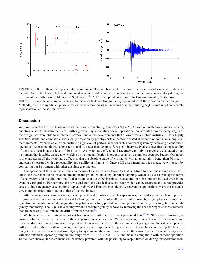
Figure 6. Left: results of the repeatability measurement. The numbers next to the points indicate the order in which data wererecorded (see Table 1 for details and numerical values). Right: gravity residuals measured in the Larzac observatory during the8.1 magnitude earthquake in Mexico on September 8th, 2017. Each point corresponds to 1 measurement cycle (approx.500 ms). Because seismic signal occurs at frequencies that are close to the high-pass cutoff of the vibration correction (seeMethods), there are significant phase shifts on the acceleration signal, meaning that the resulting AQG signal is not an accuraterepresentation of the seismic waves.

DiscussionWe have presented the results obtained with an atomic quantum gravimeter (AQG-A01) based on matter-wave interferometry,enabling absolute measurements of Earth’s gravity. By accounting for all operational constraints from the early stages ofthe design, we were able to implement several innovative developments that allowed for a mobile instrument. It is highlysensitive, stable, and compatible with a daily operation by geophysicists either for repeated short-term or continuous long-termmeasurements. We were able to demonstrate a high level of performance for such a compact system by achieving a continuousoperation over one month with a long-term stability better than 10 nm.s−2. A preliminary study also shows that the repeatabilityof the instrument is at the level of 10 nm.s−2. As systematic effects and accuracy can only be precisely evaluated on aninstrument that is stable, we are now working on their quantification in order to establish a complete accuracy budget. Our targetis to characterize all the systematic effects so that the absolute value of g is known with an uncertainty better than 50 nm.s−2

and can be measured with a repeatability and stability of 10 nm.s−2. Once a full assessment has been made, we will test it bycomparing our instrument with other absolute gravimeters.

The operation of the gravimeter relies on the use of a classical accelerometer that is utilized to filter out seismic noise. Thisallows the instrument to be installed directly on the ground without any vibration damping, which is a clear advantage in termsof size, weight and installation time. It also means that our AQG is robust to acceleration noise and can be used even in theevent of earthquakes. Furthermore, the raw signal from the classical accelerometer, which can be recorded and stored, providesaccess to high-frequency accelerations (typically above 0.1 Hz), which could prove relevant in applications where these signalsgive complementary information to that of the gravimeter.

After years of pioneering laboratory developments and proof-of-principle experiments, the results presented here representa significant advance in cold-atom-based technology and the use of matter-wave interferometry in geophysics. Simplifiedoperation and continuous data acquisition capability over long periods of time open new pathways for long-term absolutegravity monitoring. The AQG can also improve and accelerate gravity surveys by removing the need for repeated measurementsthat are necessary to eliminate the drift of relative meters38.

We believe that the limits have not yet been reached with the instrument presented here15, 16. Short-term sensitivity iscurrently limited by imperfections in the compensation of vibrations. We are working on new low-noise electronics andreal-time data processing to improve this point and to increase the SNR of the instrument. Ongoing technological developmentswill also reduce the overall size, weight and power consumption of the gravimeter. This includes increasing the level ofintegration of the electronics and simplifying the system and the connection between the various parts. Thermal managementwill also extend its operating temperature range from 18−30◦C to 0−40◦C and make it compatible with outdoor operation.To facilitate surveys, the instrument will be battery-powered, with the possibility to keep it turned on during transportation from

9/13

one site to the next. With these improvements, the AQG could be used for geophysical measurements that often take place inuncontrolled environments.

Methods

Atomic temperature measurementTo estimate the temperature of the atomic cloud, we use Raman spectroscopy. After cooling and preparation, the atoms aredropped. We drive a Raman transition with a 80 µs pulse and detect fluorescence at the bottom of the chamber. The resultingprofile is the convolution of the atomic velocity distribution by the Raman pulse width. Assuming the latter to be negligible wemeasure the full width at half maximum (FWHM) of the distribution and derive the corresponding temperature, below 2 µK.

Vibration acquisition and compensationThe signal from the classical accelerometer (Nanometrics Titan) is filtered by a bandpass filter with cut-off frequenciesfhp = 0.05 Hz and flp = 1 kHz. The high-pass filter removes any long-term drift of the accelerometer and makes sure thatthe mean gravity value only comes from the atomic measurement. fhp has been chosen much lower than the cycle frequencyof the AQG (2 Hz), so that there is no significant phase shift of the signal at 2 Hz. The low-pass filter essentially eliminateshigh-frequency electronic noise before the signal is digitized. Since the atom interferometer behaves as a second-order filterwith a low-pass cut-off frequency of 1/2T = 8.3 Hz, flp is chosen significantly higher. This way, we make sure the electroniclow-pass filter does not impact the measurement at frequencies where the atom interferometer has a residual sensitivity.

The filtered signal is digitized and weighted in real-time by the transfer function of the atom interferometer32, 41. Theacceleration response function has a simple triangle shape so the real-time calculation is straightforward. It has beendemonstrated that a convenient and yet robust way of taking into account the response function of the system is to introduce adelay on the application of the sensitivity function35. This delay is simply calculated by optimizing the signal-to-noise ratio ofthe instrument. Less than 1 ms before the last Raman pulse, the calculated correction is applied to the phase lock loop of theRaman lasers to compensate the vibration phase shift.

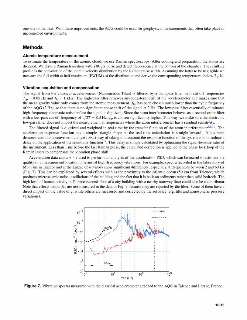
Acceleration data can also be used to perform an analysis of the acceleration PSD, which can be useful to estimate thequality of a measurement location in terms of high-frequency vibrations. For example, spectra recorded in the laboratory ofMuquans in Talence and at the Larzac observatory show significant differences, especially at frequencies between 2 and 60 Hz(Fig. 7). This can be explained by several effects such as the proximity to the Atlantic ocean (50 km from Talence) whichproduces microseismic noise, oscillations of the building and the fact that it is built on sediments rather than solid bedrock. Thehigh level of human activity in Talence (second-floor of a city building with a nearby tramway line) could also be a contributor.Note that effects below fhp are not measured in the data of Fig. 7 because they are rejected by the filter. Some of them have adirect impact on the value of g, while others are measured and corrected by the software (e.g. tilts and atmospheric pressurevariations).

Figure 7. Vibration spectra measured with the classical accelerometer attached to the AQG in Talence and Larzac, France.

10/13

Linewidth and long-term frequency stability measurementWe record the beatnote between the laser of the AQG and a similar independent laser to estimate the linewidth and frequencystability of the gravimeter laser. The two lasers are in a master / slave configurations, so they have adjustable setpoints. Wetypically use a frequency difference on the order of 80 MHz.

The beatnote is recorded on a fast photodiode and sent to an RF spectrum analyzer. The center of the spectrum can befitted by a Gaussian function accounting for technical noise. The tails (more than 5σ away from the center) are fitted by aLorentzian function. Assuming the two lasers to be independent, the width of the fitted function is the sum of the two individualwidths. Also assuming the two lasers to be identical, we estimate their linewidth as half of this. In the case of Fig. 2, the fittedLorentzian width is 23.2 kHz, meaning that both lasers have a linewidth of less than 12 kHz.

To measure the long-term frequency stability, the beatnote signal is sent to a frequency counter and compared to a stable RFreference. We measure the standard deviation of the beatnote frequency and expect that each of the two lasers has a stabilitylower than this value (27 kHz in the case of Fig. 2). Assuming similarity and independence of the two lasers as above, thiscorresponds to a worst-case estimation.

Tiltmeter offset correctionWe measure the offset of the tiltmeters by performing an in-situ calibration that also takes into account any additional angle dueto imperfect alignments between the tiltmeters and the pyramid reflector. This calibration only has to be performed once, afterassembling the sensor head.

We apply known tilts in both directions to the instrument and measure the resulting value of gravity. Applied tilts typicallyrange from 0 to 1.5 mrad, corresponding to gravity variations of approximately 10 µm.s−2. We fit the data to find the positionof the maximum, that corresponds to verticality.

The measurement sensitivity is limited by statistical uncertainties on the values of g, giving an estimation of the tiltmeteroffsets with a precision lower than 10 µrad. This is sufficient to ensure that tilts can be corrected from the final gravitymeasurements with a precision better than 10 nm.s−2.

Sensitivity estimationWe use the Allan deviation and PSD of the data to estimate the sensitivity and stability of the instrument42.

The data we obtain from both the AQG and the FG5 display a classical white noise behaviour over a large frequency range.In this regime, the Allan deviation decreases in proportion with the square root of the averaging time τ . In the log-log plot ofFig. 5 this behaviour is characterized by a linear decrease with a slope of −1/2. The sensitivity S of the instrument, expressedin nm.s−2.Hz−1/2, is the extrapolation of the white noise behaviour to τ = 1 s. This can be conveniently interpreted as thestatistical uncertainty obtained after averaging data over 1 s.

In the Allan deviation plot, all three data sets exhibit a clear white-noise signature between 100 and 2000 s. The correspond-ing sensitivities are indicated by the dashed lines: approximately 450 nm.s−2.Hz−1/2 for the FG5 and 750 nm.s−2.Hz−1/2 forthe AQG measurement in Larzac. In the PSD plot, this corresponds to constant levels between 5×10−4 and 1×10−2 Hz. Thevalue S of the PSD (expressed in (nm.s−2)2.Hz−1) in this white noise region is related to the sensitivity by42

S = 2×S 2. (5)

At longer timescales, both the PSD and Allan deviation show that the data can no longer be described as white noise,indicating instrumental drifts or long-term geophysical effects1.

Data availabilityThe datasets generated during and/or analysed during the current study are available from the corresponding author onreasonable request.

References1. Van Camp, M. et al. Geophysics from terrestrial time-variable gravity measurements. Rev. Geophys. 55, 938–992 (2007).

2. Makinen, J., Amalvict, M., Shibuya, K. & Fukuda, Y. Absolute gravimetry in Antarctica: Status and prospects. J. Geodyn.43, 339 – 357 (2007).

3. Van Dam, T. et al. Using GPS and absolute gravity observations to separate the effects of present-day and pleistoceneice-mass changes in south east Greenland. Earth Planet. Sci. Lett. 459, 127 – 135 (2017).

4. Carbone, D., Poland, M. P., Diament, M. & Greco, F. The added value of time-variable microgravimetry to the understandingof how volcanoes work. Earth-Science Rev. 169, 146 – 179 (2017).

11/13

5. Kennedy, J., Ferre, T. P. A. & Creutzfeldt, B. Time-lapse gravity data for monitoring and modeling artificial rechargethrough a thick unsaturated zone. Water Resour. Res. 52, 7244–7261 (2016).

6. Fores, B., Champollion, C., Le Moigne, N., Bayer, R. & Chery, J. Assessing the precision of the iGrav superconductinggravimeter for hydrological models and karstic hydrological process identification. Geophys. J. Int. 208, 269–280 (2017).

7. Van Camp, M. et al. Repeated absolute gravity measurements for monitoring slow intraplate vertical deformation inwestern Europe. J. Geophys. Res. Solid Earth 116, B08402 (2011).

8. Pearson-Grant, S., Franz, P. & Clearwater, J. Gravity measurements as a calibration tool for geothermal reservoir modelling.Geothermics 73, 146 – 157 (2018).

9. Romaides, A. J. et al. A comparison of gravimetric techniques for measuring subsurface void signals. J. Phys. D: Appl.Phys. 34, 433 (2001).

10. Niebauer, T. M., Sasagawa, G. S., Faller, J. E., Hilt, R. & Klopping, F. A new generation of absolute gravimeters. Metrol.32, 159 (1995).

11. Kasevich, M. & Chu, S. Atomic interferometry using stimulated Raman transitions. Phys. Rev. Lett. 67, 181–184 (1991).

12. Peters, A., Chung, K. Y. & Chu, S. Measurement of gravitational acceleration by dropping atoms. Nat. 400, 849 (1999).

13. Pereira Dos Santos, F. & Bonvalot, S. Cold-Atom Absolute Gravimetry, in Encyclopedia of Geodesy, (ed. Grafarend E.)1–6 (Springer International Publishing, 2016).

14. Gillot, P., Francis, O., Landragin, A., Pereira Dos Santos, F. & Merlet, S. Stability comparison of two absolute gravimeters:optical versus atomic interferometers. Metrol. 51, L15 (2014).

15. Farah, T. et al. Underground operation at best sensitivity of the mobile LNE-SYRTE cold atom gravimeter. GyroscopyNavig. 5, 266–274 (2014).

16. Freier, C. et al. Mobile quantum gravity sensor with unprecedented stability. J. Physics: Conf. Ser. 723, 012050 (2016).

17. Min-Kang, Z. et al. Micro-gal level gravity measurements with cold atom interferometry. Chin. Phys. B 24, 050401 (2015).

18. Jiang, Z. et al. The 8th international comparison of absolute gravimeters 2009: the first key comparison (CCM.G-K1) inthe field of absolute gravimetry. Metrol. 49, 666 (2012).

19. Francis, O. et al. The european comparison of absolute gravimeters 2011 (ECAG-2011) in Walferdange, Luxembourg:results and recommendations. Metrol. 50, 257 (2013).

20. Wang, S. et al. Shift evaluation of the atomic gravimeter NIM-AGRb-1 and its comparison withFG5X. Metrol. (2018).

21. Bidel, Y. et al. Compact cold atom gravimeter for field applications. Appl. Phys. Lett. 102, 144107 (2013).

22. Wu, B. et al. The investigation of a microgal-level cold atom gravimeter for field applications. Metrol. 51, 452 (2014).

23. Bidel, Y. et al. Absolute marine gravimetry with matter-wave interferometry. Nat. Commun. 9, 627; 10.1038/s41467-018-03040-2 (2018).

24. Bodart, Q. et al. A cold atom pyramidal gravimeter with a single laser beam. Appl. Phys. Lett. 96, 134101 (2010).

25. Bouyer, P. & Landragin, A. Cold atom interferometry sensor, Patent WO 2009/118488 A2 (2009).

26. Steck, D. A. Rubidium 87 D line data http://steck.us/alkalidata/rubidium87numbers.pdf (2015).

27. Borde, C. Atomic interferometry with internal state labelling. Phys. Lett. A 140, 10 – 12 (1989).

28. Kasevich, M. et al. Atomic velocity selection using stimulated Raman transitions. Phys. Rev. Lett. 66, 2297–2300 (1991).

29. Louchet-Chauvet, A. et al. The influence of transverse motion within an atomic gravimeter. New J. Phys. 13, 065025(2011).

30. Leveque, T., Antoni-Micollier, L., Faure, B. & Berthon, J. A laser setup for rubidium cooling dedicated to spaceapplications. Appl. Phys. B 116, 997–1004 (2014).

31. Theron, F. et al. Narrow linewidth single laser source system for onboard atom interferometry. Appl. Phys. B 118, 1–5(2015).

32. Cheinet, P. et al. Measurement of the sensitivity function in a time-domain atomic interferometer. IEEE Transactions onInstrumentation Meas. 57, 1141–1148 (2008).

33. Trimeche, A., Langlois, M., Merlet, S. & Pereira Dos Santos, F. Active control of laser wavefronts in atom interferometers.Phys. Rev. Appl. 7, 034016 (2017).

12/13

34. Merlet, S. et al. Operating an atom interferometer beyond its linear range. Metrol. 46, 87 (2009).

35. Lautier, J. et al. Hybridizing matter-wave and classical accelerometers. Appl. Phys. Lett. 105, 144102 (2014).

36. Van Camp, M. & Vauterin, P. Tsoft: graphical and interactive software for the analysis of time series and Earth tides.Comput. & Geosci. 31, 631 – 640 (2005).

37. Hinderer, J. et al. A search for atmospheric effects on gravity at different time and space scales. J. Geodyn. 80, 50 – 57(2014).

38. Jacob, T., Bayer, R., Chery, J. & Le Moigne, N. Time-lapse microgravity surveys reveal water storage heterogeneity of akarst aquifer. J. Geophys. Res. Solid Earth 115, B06402 (2010).

39. Van Camp, M., Williams, S. D. P. & Francis, O. Uncertainty of absolute gravity measurements. J. Geophys. Res. SolidEarth 110, B05406 (2005).

40. Peterson, J. Observations and modeling of seismic background noise. https://pubs.usgs.gov/of/1993/0322/report.pdf. (USGS Open-3034 File No. 93–322). U.S. Department of Interior Geological Survey (1993).

41. Geiger, R. et al. Detecting inertial effects with airborne matter-wave interferometry. Nat. Commun. 2, 474;10.1038/ncomms1479 (2011).

42. Riley, W. J. Handbook of frequency stability analysis. https://tf.nist.gov/general/pdf/2220.pdf. NISTspecial publication 1065 (2008).

AcknowledgementsDevelopment of the AQG was funded through the EquipEx RESIF-CORE which is supported by a public grant overseen bythe French national research agency (ANR) as part of the Investissements d’Avenir program (ANR-11-EQPX-0040). We alsoacknowledge support from Direction Generale de l’Armement (GRAVITER project), Region Aquitaine and Idex Universitede Toulouse, IRD and CNRS (GEOMIP project). The authors acknowledge a major contribution from the Muquans team inthe design, integration, characterization and optimization of the Absolute Quantum Gravimeter. They thank Franck PereiraDos Santos and Sebastien Merlet for helpful discussions, and Baptiste Battelier for his support in the early-stage design of theinstrument.

13/13