10 OD Decision Analysis-2009 - Técnico Lisboa ... OD... · Introduction Decision often must be made in uncertain environments Examples: Manufacturer introducing a new product in

DECISION ANALYSIS

(Hillier & Lieberman Introduction to Operations Research, 8th edition)

Introduction

f b dDecision often must be made in uncertain environmentsExamples:

Manufacturer introducing a new product in the marketplace.Government contractor bidding on a new contract.Oil company deciding to drill for oil in a particular location.

Decision analysis: decision making in face of great Decision analysis: decision making in face of great uncertainty; rational decision when the outcomes are uncertain.uncertain.Making decisions with or without experimentation.

Optimization and Decision 2009 530

Prototype exampleyp p

Goferbroke Company owns a tract of land that can Goferbroke Company owns a tract of land that can contain oil.

Contracted geologist reports that chance of oil is 1 in 4Contracted geologist reports that chance of oil is 1 in 4.Another oil company offers 90.000€ for the land.Cost of drilling is 100 000€ If oil is found expected revenue Cost of drilling is 100.000€. If oil is found, expected revenue is 800.000€ (expected profit is 700.000€).

Status of land Alternative

Payoff

Oil Dry

D ill f ilDrill for oil 700.000€ –100.000€

Sell the land 90.000€ 90.000€

Chance of status 1 in 4 3 in 4Chance of status 1 in 4 3 in 4


Decision making without experimentationg p

l hAnalogy to game theory:Players: decision maker (player 1) and nature (player 2). Available strategies for 2 players: alternative actions and possible states of nature, respectively.

f ffCombination of strategies results in some payoff to player 1 (decision maker).

But, are both players still rational?


Decision analysis frameworky

1. Decision maker needs to choose one of alternative actions.

2. Nature then chooses one of possible states of nature.p f3. Each combination of an action and state of nature

results in a payoff one of the entries in a payoff results in a payoff, one of the entries in a payoff table.

4 Probabilities for states of nature provided by prior 4. Probabilities for states of nature provided by prior distribution are prior probabilities.P ff t bl h ld b d t fi d ti l ti5. Payoff table should be used to find an optimal actionfor the decision maker according to an appropriateit icriterion.


Payoff table for Goferbroke Co. problemy p

State of natureAlternative Oil Dry

1 Drill for oil 700 1001. Drill for oil 700 –100

2. Sell the land 90 90

Prior probability 0.25 0.75


Maximin payoff criterionp y

Maximin payoff criterion: for each possible action, find the minimum payoff over all states of nature. Next, find the maximum of these minimum payoffs. Choose the action whose minimum payoff gives this maximum.Best guarantee of payoff: pessimistic viewpoint.

St t f tAlternative

State of nature

Oil Dry Minimum

1 Drill for oil 700 –100 –1001. Drill for oil 700 –100 –100

2. Sell the land 90 90 90 ←Maximin value

Prior probability 0.25 0.75Prior probability 0.25 0.75


Maximum likelihood criterion

Maximum likelihood criterion: Identify most likelystate of nature (with largest prior probability). For this state of nature, find the action with maximum payoff. Choose this action.Most likely state: ignores important information and y g plow‐probability big payoff.

State of natureAlternative

State of nature

Oil Dry

1. Drill for oil 700 –100

2. Sell the land 90 90 ←Maximum in this column

Prior probability 0.25 0.75

↑Most likelyOptimization and Decision 2009 536

Bayes’ decision ruley

Bayes’ decision rule: Using prior probabilities, Bayes decision rule: Using prior probabilities, calculate the expected value of payoff for each possible decision alternative. Choose the decision possible decision alternative. Choose the decision alternative with the maximum expected payoff.For the prototype example:For the prototype example:

E[Payoff (drill)] = 0.25(700) + 0.75(–100) = 100.E[Payoff (sell)] 0 25(90) + 0 75(90) 90E[Payoff (sell)] = 0.25(90) + 0.75(90) = 90.

Incorporates all available information (payoffs and i b biliti )prior probabilities).

What if probabilities are wrong?


Sensitivity analysis with Bayes’ rulesy y y

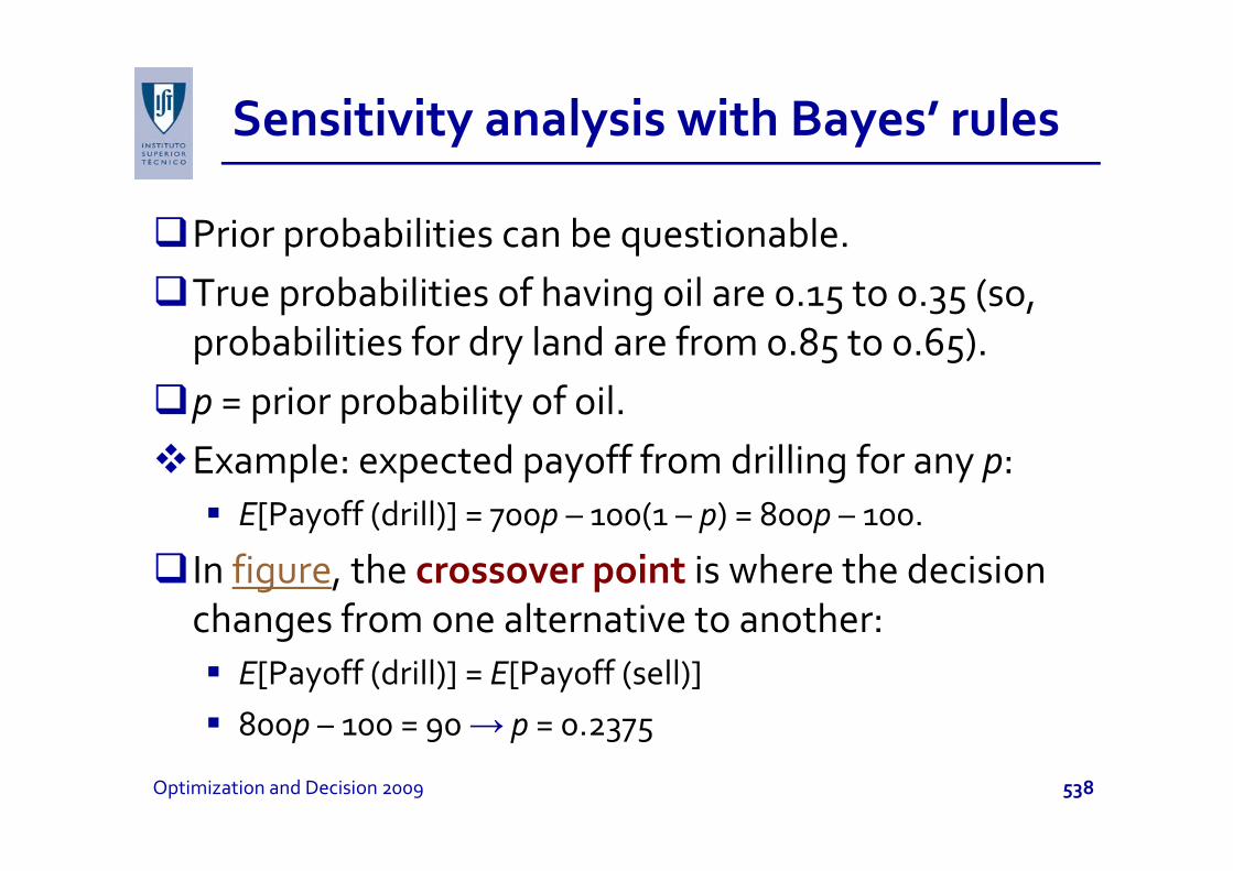
Prior probabilities can be questionablePrior probabilities can be questionable.True probabilities of having oil are 0.15 to 0.35 (so, probabilities for dry land are from 0 85 to 0 65)probabilities for dry land are from 0.85 to 0.65).p = prior probability of oil.Example: expected payoff from drilling for any p:

E[Payoff (drill)] = 700p – 100(1 – p) = 800p – 100.

In figure, the crossover point is where the decision changes from one alternative to another:g

E[Payoff (drill)] = E[Payoff (sell)]800p – 100 = 90 → p = 0.2375800p 100 90 → p 0.2375


Expected payoff for alternative changesp p y g

And for more And for more than 2 variables?Use Excel SensIt.

The decision is very sensitive very sensitive

to p!


Decision making with experimentationg p

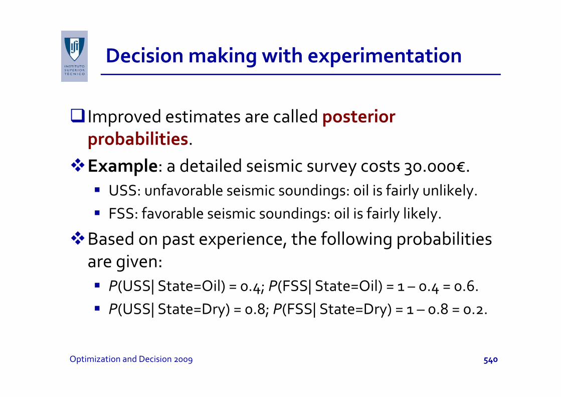
Improved estimates are called posterior probabilities.Example: a detailed seismic survey costs 30.000€.

USS: unfavorable seismic soundings: oil is fairly unlikely.g y yFSS: favorable seismic soundings: oil is fairly likely.

Based on past experience, the following probabilities Based on past experience, the following probabilities are given:

P(USS| State=Oil) = 0 4; P(FSS| State=Oil) = 1 – 0 4 = 0 6P(USS| State=Oil) = 0.4; P(FSS| State=Oil) = 1 0.4 = 0.6.P(USS| State=Dry) = 0.8; P(FSS| State=Dry) = 1 – 0.8 = 0.2.


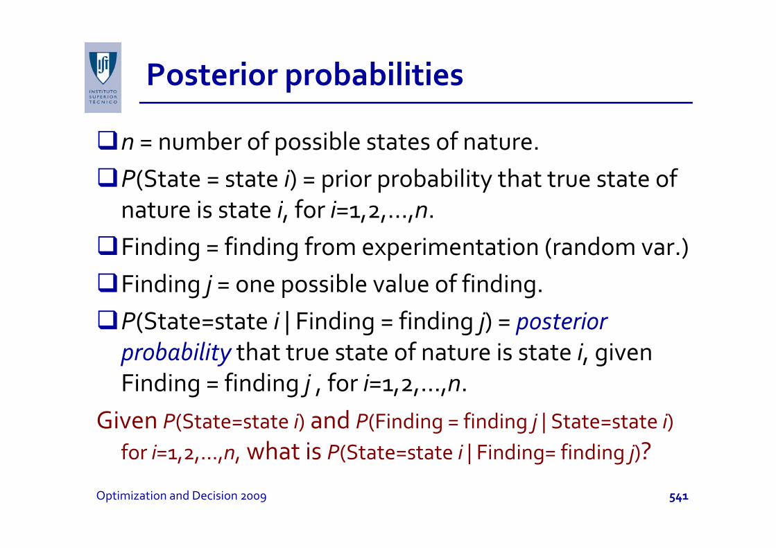
Posterior probabilitiesp

n = number of possible states of nature.u be o poss b e states o atu eP(State = state i) = prior probability that true state of nature is state i for i=1 2 nnature is state i, for i=1,2,…,n.Finding = finding from experimentation (random var.)

d bl l f f dFinding j = one possible value of finding.P(State=state i | Finding = finding j) = posterior probability that true state of nature is state i, given Finding = finding j , for i=1,2,…,n.

Given P(State=state i) and P(Finding = finding j | State=state i)for i=1,2,…,n, what is P(State=state i | Finding= finding j)?, , , , ( | g g j)


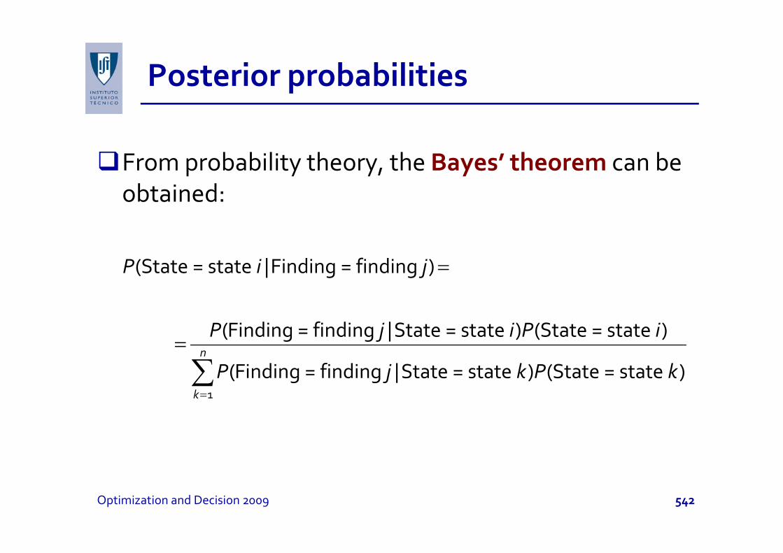
Posterior probabilitiesp

From probability theory, the Bayes’ theorem can be obtained:

(State = state |Finding = finding )P i j =| g g

(Finding = finding |State = state ) (State = state )

j

P j i P i

1

( g g | ) ( )

(Finding = finding |State = state ) (State = state )n

k

j

P j k P k=

=

∑


Bayes’ theorem in prototype exampley p yp p

If seismic survey in unfavorable (USS j=1):If seismic survey in unfavorable (USS, j=1):0.4(0.25) 1

(State = Oil | Finding = USS) ,0 4(0 25) 0 8(0 75) 7

P = =+0.4(0.25) 0.8(0.75) 7+

1 6(State = Dry | Finding = USS) 1 .P = − =

If seismic survey in favorable (FSS , j=2):

y | g7 7

0.6(0.25) 1(State = Oil | Finding = FSS) ,

0.6(0.25) 0.2(0.75) 2P = =

+

1 1(State = Dry | Finding = FSS) 1 .

2 2P = − =


Probability tree diagramy g


Expected payoffsp p y

Expected payoffs can be found again using Bayes’ decision rule for the prototype example, with posterior probabilities replacing prior probabilities:Expected payoffs if finding is USS:

1 6[Payoff (drill | Finding = USS) (700) ( 100) 3 10 5.7E = − =−+[ y ( | g ) (7 ) ( ) 3

75 7

71 6

[Payoff (sell | Finding = USS) (90) (90) 607 7

30E −= + =

Expected payoffs if finding is FSS:7 7

1 1[Payoff (drill | Finding FSS) (700) ( 100) 2730 0E +[Payoff (drill | Finding = FSS) (700) ( 100) 2730 0

2 2E −= + − =

1 1[Payoff (sell | Finding = FSS) (90) (90) 6030E −= + =[ y ( | g ) (9 ) (9 )

2 23


Optimal policyp p y

Using Bayes’ decision rule, the optimal policy of optimizing payoff is given by:

Finding from Optimal Expected payoff Expected payoff

Finding from seismic survey

Optimal alternative

excluding cost of survey

including cost of survey

USS Sell the land 90 60USS Se t e a d 90 60

FSS Drill for oil 300 270

Is it worth spending 30.000€ to conduct the experimentation?


p

Value of experimentationp

Before performing an experimentation, determine its potential value.Two complementary methods:

1. Expected value of perfect information – it is 1. Expected value of perfect information it is assumed that experiment will remove all uncertainty. Provides an upper bound on potential value of o des a uppe bou d o pote t a a ue oexperiment.

2 Expected value of information – is the actual2. Expected value of information – is the actualimprovement in expected payoff.


Expected value of perfect informationp p

State of natureState of nature

Alternative Oil Dry

1. Drill for oil 700 –100

2. Sell the land 90 90

Maximum payoff 700 90

P i b biliPrior probability 0.25 0.75

Expected payoff with perfect information = 0.25(700) + 0.75(90) = 242.5

Expected value of perfect information (EVPI) is:EVPI = expected payoff with perfect information – expected payoff without

experimentation

Example: EVPI = 242.5 – 100 = 142.5. This value is > 30.


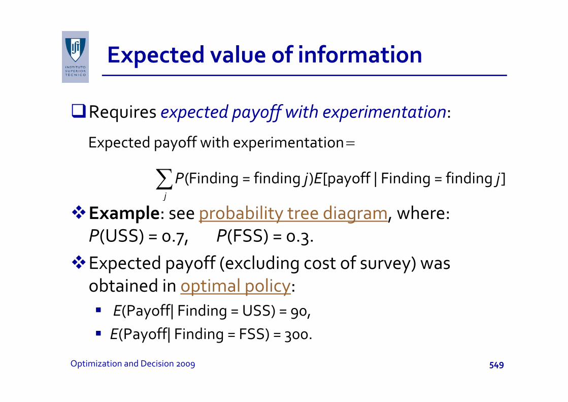
Expected value of informationp

Requires expected payoff with experimentationRequires expected payoff with experimentation:

Expected payoff with experimentation=

(Finding = finding ) [payoff | Finding = finding ]j

P j E j∑Example: see probability tree diagram, where: P(USS) = 0.7, P(FSS) = 0.3.Expected payoff (excluding cost of survey) was obtained in optimal policy:p p y

E(Payoff| Finding = USS) = 90,E(Payoff| Finding = FSS) = 300.E(Payoff| Finding FSS) 300.


Expected value of informationp

So, expected payoff with experimentation isExpected payoff with experim. = 0.7(90) + 0.3(300) = 153.

Expected value of experimentation (EVE) is:EVE = expected payoff with experimentation – expected

payoff without experimentation

Example: EVE = 153 – 100 = 53.As 53 exceeds 30, the seismic survey should be done.


Decision trees

P l h f d i iPrototype example has a sequence of two decisions:Should a seismic survey be conducted before an action is h ?chosen?Which action (drill for oil or sell the land) should be chosen?h h d dThese questions have a corresponding decision tree.

Junction points are nodes, and lines are branches.A decision node, represented by a square, indicates that a decision needs to be made at that point.pAn event node, represented by a circle, indicates that a random event occurs at that point.a random event occurs at that point.


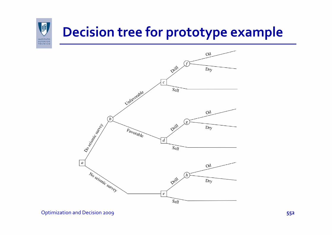
Decision tree for prototype examplep yp p


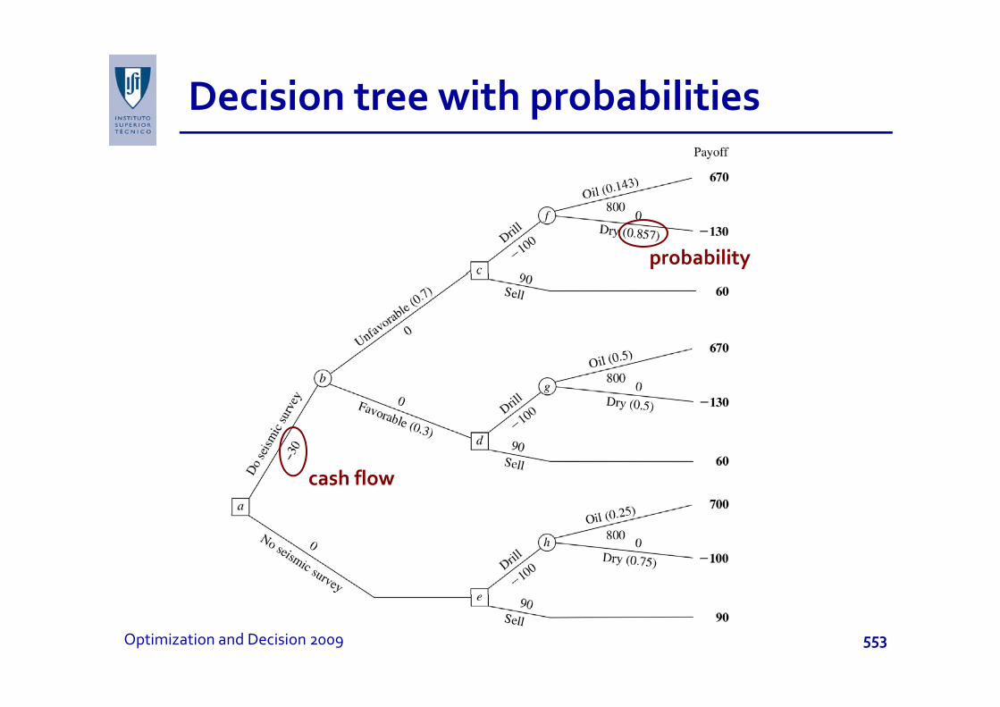
Decision tree with probabilitiesp

probability

cash flow


Performing the analysisg y

1. Start at right side of decision tree and move left one 1. Start at right side of decision tree and move left one column at a time. For each column, perform step 2 or step 3 depending if nodes are event or decision nodes.step 3 depending if nodes are event or decision nodes.

2. For each event node, calculate its expected payoff by multiplying expected payoff of each branch by multiplying expected payoff of each branch by probability of that branch and summing these products Record value next to each node in boldproducts. Record value next to each node in bold.

3. For each decision node, compare the expected payoffs f it b h d h lt ti ith l t of its branches, and choose alternative with largest

expected payoff. Record the choice by inserting a d bl d h i h j t d b hdouble dash in each rejected branch.


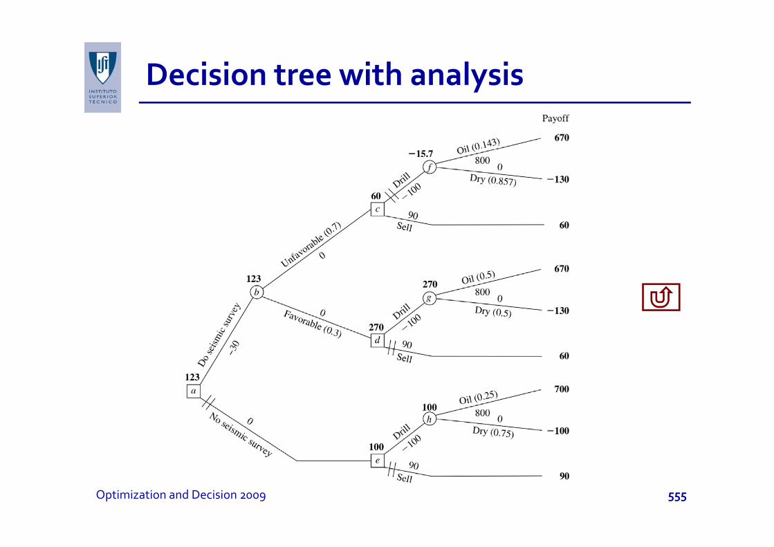
Decision tree with analysisy


Optimal policy for prototype examplep p y p yp p

The decision tree results in the following decisions:The decision tree results in the following decisions:1. Do the seismic survey.

If h l i f bl ll h l d2. If the result is unfavorable, sell the land.3. If the result is favorable, drill for oil.4. The expected payoff (including the cost of the

seismic survey) is 123 (123 000€).y) 3 ( 3 )

Same result as obtained with experimentationFor any decision tree, the backward induction procedure always leads to optimal policy.


Utility theoryy y

You are offered the choice of:

1. Accepting a 50:50 chance of winning $100.000 or nothing;or nothing;

2. Receiving $40.000 with certainty.

What do you choose?


Utility function for moneyy y

Utility functions (u(M)) for money (M): usually there is a d i i l ili f (i di id l i i kdecreasing marginal utility for money (individual is risk‐averse).


Utility function for moneyy y

It also is possible to exhibit a mixture of these kinds of pbehavior (risk‐averse, risk seeker, risk‐neutral)An individual’s attitude toward risk may be different An individual s attitude toward risk may be different when dealing with one’s personal finances than when making decisions on behalf of an organization.making decisions on behalf of an organization.When a utility function for money is incorporated into a decision analysis approach to a problem this utility a decision analysis approach to a problem, this utility function must be constructed to fit the preferences and values of the decision maker involved (The and values of the decision maker involved. (The decision maker can be either a single individual or a group of people )group of people.)


Utility theoryy y

Fundamental property: the decision maker’s utility Fundamental property: the decision maker s utility function for money has the property that the decision maker is indifferent between two alternative courses ffof action if they have the same expected utility.Example. Offer: an opportunity to obtain either p pp y$100.000 (utility = 4) with probability p or nothing (utility = 0) with probability 1 – p. Thus, E(utility) = 4p.

Decision maker is indifferent for e.g.:Offer with p = 0.25 (E(utility) = 1) or definitely obtaining $ 0 000 ( tilit )$10.000 (utility = 1).Offer with p = 0.75 (E(utility) = 3) or definitely obtaining $60.000 (utility = 3).$60.000 (utility 3).


Role of utility theoryy y

When decision maker’s utility function for money is used to measure relative worth of various possible monetary outcomes, Bayes’ decision rule replaces monetary payoffs by corresponding utilities. Thus, optimal action is the one that maximizes the expected utility.

Note that utility functions may not be monetary.Example: doctor’s decision of treating or not a patient involves future health of the patient.


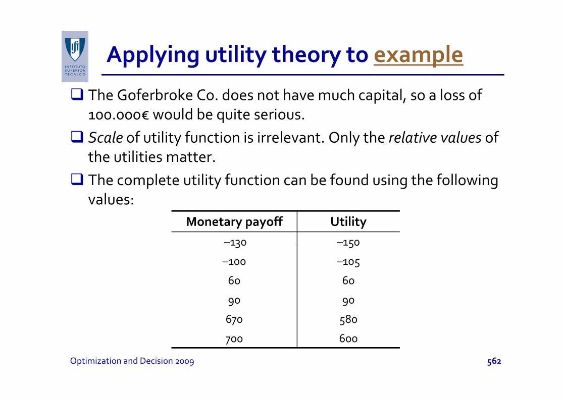
Applying utility theory to examplepp y g y y p

The Goferbroke Co. does not have much capital, so a loss of ld b i i100.000€ would be quite serious.

Scale of utility function is irrelevant. Only the relative values of the tilities matterthe utilities matter.The complete utility function can be found using the following values:values:

Monetary payoff Utility–130 –150130 150

–100 –105

60 60

90 90

670 580

6700 600


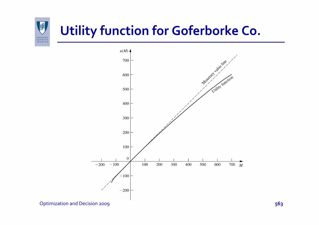
Utility function for Goferborke Co.y


Estimating u(M)g ( )

A popular form is the exponential utility function:

( )MRM R

−⎛ ⎞⎜ ⎟

R = decision maker’s risk tolerance

( ) 1 Ru M R e= −⎜ ⎟⎝ ⎠

R = decision maker s risk tolerance.Designed to fit a risk‐averse individual.

F l R f (6 ) 8 d For prototype example, R = 2250 for u(670) = 580 and u(700) = 600, and R = 465 for u(–130) = –150.

H it i t ibl t h diff t l f However, it is not possible to have different values of R for the same utility function.


Decision tree with utility functiony

The solution is exactly the same as before, except for substituting utilities for monetary payoffs.Thus, the value obtained to evaluate each fork of the tree is now the expected utility rather than the yexpected monetary payoff.Optimal decisions selected by Bayes’ decision rule Opt a dec s o s se ected by ayes dec s o u emaximize the expected utility for the overall problem.


Decision tree using utility functiong y

Different decision treebut same optimalpolicy.


Documents

10 OD Decision Analysis-2009 - Técnico Lisboa ... OD... · Introduction Decision often must be made in uncertain environments Examples: Manufacturer introducing a new product in