Embed Size (px)
Citation preview

Dr. Rakhesh Singh Kshetrimayum
10. Method of Moments
Dr. Rakhesh Singh Kshetrimayum
1/3/20141 Electromagnetic Field Theory by R. S. Kshetrimayum
10.1 Introduction
� learn how to use method of moments (MoM) to solve� electrostatic problems
� advanced & challenging problems in time-varying fields
� brief discussion on the basic steps of MoM
� solve a simple differential equation using MoM
1/3/2014Electromagnetic Field Theory by R. S. Kshetrimayum2
� solve a simple differential equation using MoM� in order to elucidate the steps involved
� MoM tfor 1-D and 2-D electrostatic problems
� MoM for electrodynamic problems

10.2 Basic Steps in Method of Moments
� Method of Moments (MoM) transforms � integro-differential equations into matrix systems of linear equations
� which can be solved using computers
� Consider the following inhomogeneous equation
( ) kuL =
1/3/2014Electromagnetic Field Theory by R. S. Kshetrimayum3
� where L is a linear integro-differential operator,
� u is an unknown function (to be solved) and
� k is a known function (excitation)
( ) kuL =
( ) 0=−⇒ kuL

10.2 Basic Steps in Method of Moments
� For example,
� (a) consider the integral equation for a line charge density
Then
0
0
( ') '
4 ( , ')
x dxV
r x x
λ
πε= ∫
( )
1/3/2014Electromagnetic Field Theory by R. S. Kshetrimayum4
� Then ( )'u xλ=
0k V=
0
'
4 ( , ')
dxL
r x xπε= ∫
10.2 Basic Steps in Method of Moments
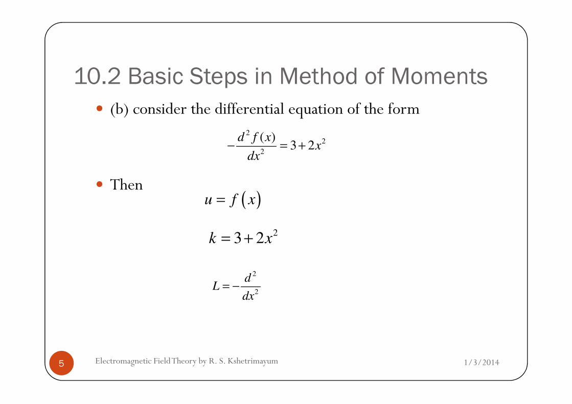
� (b) consider the differential equation of the form
� Then
22
2
( )3 2
d f xx
dx− = +
( )u f x=
1/3/2014Electromagnetic Field Theory by R. S. Kshetrimayum5
( )u f x=
23 2k x= +
2
2
dL
dx= −

10.2 Basic Steps in Method of Moments
� To solve u, approximate it by sum of weighted known � basis functions or
� expansion functions
� as given belowN N
≅ = =∑ ∑
1/3/2014Electromagnetic Field Theory by R. S. Kshetrimayum6
� where is the expansion function,
� is its unknown complex coefficients to be determined,
� N is the total number of expansion functions
1 1
, 1, 2,...,N N
n n n
n n
u u I b n N= =
≅ = =∑ ∑
nb
nI

10.2 Basic Steps in Method of Moments� Since L is linear, substitution of the above equation in the
� integro-differential equation,
� we get,
1
N
n n
n
L I b k=
≈
∑
1/3/2014Electromagnetic Field Theory by R. S. Kshetrimayum7
� where the error or residual is given by
1n= ∑
1
N
n n
n
R k L I b=
= −
∑

10.2 Basic Steps in Method of Moments
� Mathematicians name this method as Method of Weighted Residuals
� Why?
� Next step in MoM
� Enforcing the boundary condition
1/3/2014Electromagnetic Field Theory by R. S. Kshetrimayum8
� Enforcing the boundary condition
� Make inner product of the above equation with each of the � testing or
� weighting functions
� should make residual or error zero

10.2 Basic Steps in Method of Moments
� By replacing u by � where n=1,2,…,N
� taking inner product with a set of � weighting or
nu
mw
1/3/2014Electromagnetic Field Theory by R. S. Kshetrimayum9
� weighting or
� testing functions
� in the range of L, we have,
( )( ), 0, 1,2,...,m nw L u k m M− = =

10.2 Basic Steps in Method of Moments
� Since In is a constant
� we can take it outside the inner product and
� write
1/3/2014Electromagnetic Field Theory by R. S. Kshetrimayum10
� M and N should be infinite theoretically � but practically it should be a finite number
( )1
, , , 1, 2,...,N
n m n m
n
I w L b w k m M=
= =∑

10.2 Basic Steps in Method of Moments� Note that a scalar product is defined to be a scalar satisfying
, , ( ) ( )w g g w g x w x dx= = ∫
wgcwfbwcgbf ,,, +=+
gw,
1/3/2014Electromagnetic Field Theory by R. S. Kshetrimayum11
� b and c are scalars and * indicates complex conjugation
wgcwfbwcgbf ,,, +=+
00,* ≠> gifgg 00,* == gifgg

10.2 Basic Steps in Method of Moments
� In matrix form
� with each matrix and vector defined by
[ ][ ] [ ]VIZ =
[ ] [ ]TNIIII ...21= [ ] 1 2, , ... ,T
MV k w k w k w =
1/3/2014Electromagnetic Field Theory by R. S. Kshetrimayum12
[ ]
( ) ( ) ( )
( ) ( ) ( )
( ) ( ) ( )
( ) ( ) ( )
1 1 1 2 1
2 1 2 2 2
3 1 3 2 3
1 2
, , ,
, , ... ,
, , ,...
, , ... ,
N
N
N
M M M N
w L b w L b w L b
w L b w L b w L b
Z w L b w L b w L b
w L b w L b w L b
=
K
OM M M

10.2 Basic Steps in Method of Moments
� For [Z] is non-singular,
� Solve the unknown matrix [I] of amplitudes of basis function as
� Galerkin’s method
[ ] [ ] [ ] [ ][ ]1
I Z V Y V−
= =
1/3/2014Electromagnetic Field Theory by R. S. Kshetrimayum13
� Galerkin’s method
� Point matching or Collocation � The testing function is a delta function
nn wb =
10.2 Basic Steps in Method of Moments
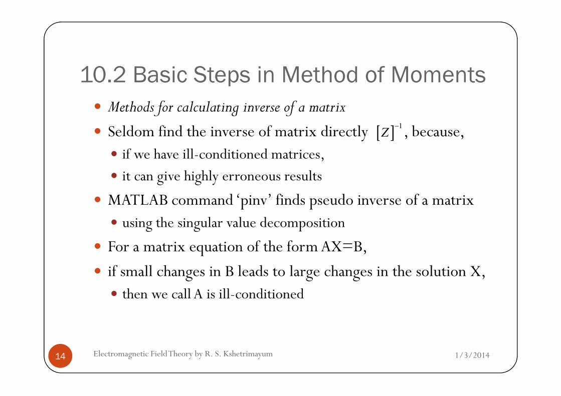
� Methods for calculating inverse of a matrix
� Seldom find the inverse of matrix directly , because, � if we have ill-conditioned matrices,
� it can give highly erroneous results
� MATLAB command ‘pinv’ finds pseudo inverse of a matrix
[ ]1
Z−
1/3/2014Electromagnetic Field Theory by R. S. Kshetrimayum14
� MATLAB command ‘pinv’ finds pseudo inverse of a matrix� using the singular value decomposition
� For a matrix equation of the form AX=B,
� if small changes in B leads to large changes in the solution X, � then we call A is ill-conditioned
10.2 Basic Steps in Method of Moments
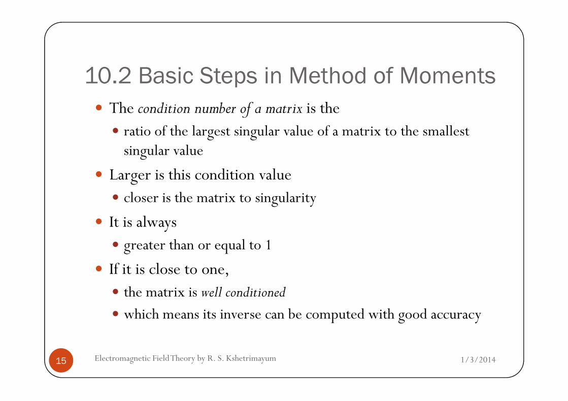
� The condition number of a matrix is the � ratio of the largest singular value of a matrix to the smallest singular value
� Larger is this condition value� closer is the matrix to singularity
1/3/2014Electromagnetic Field Theory by R. S. Kshetrimayum15
� closer is the matrix to singularity
� It is always � greater than or equal to 1
� If it is close to one, � the matrix is well conditioned
� which means its inverse can be computed with good accuracy

10.2 Basic Steps in Method of Moments
� If the condition number is large, � then the matrix is said to be ill-conditioned
� Practically, � such a matrix is almost singular, and
� the computation of its inverse, or
1/3/2014Electromagnetic Field Theory by R. S. Kshetrimayum16
� the computation of its inverse, or
� solution of a linear system of equations is � prone to large numerical errors
� A matrix that is not invertible � has the condition number equal to infinity

10.2 Basic Steps in Method of Moments
� Sometimes pseudo inverse is also used for finding � approximate solutions to ill-conditioned matrices
� Preferable to use LU decomposition � to solve linear matrix equations
� LU factorization unlike Gaussian elimination,
1/3/2014Electromagnetic Field Theory by R. S. Kshetrimayum17
� LU factorization unlike Gaussian elimination, � do not make any modifications in the matrix B
� in solving the matrix equation
10.2 Basic Steps in Method of Moments
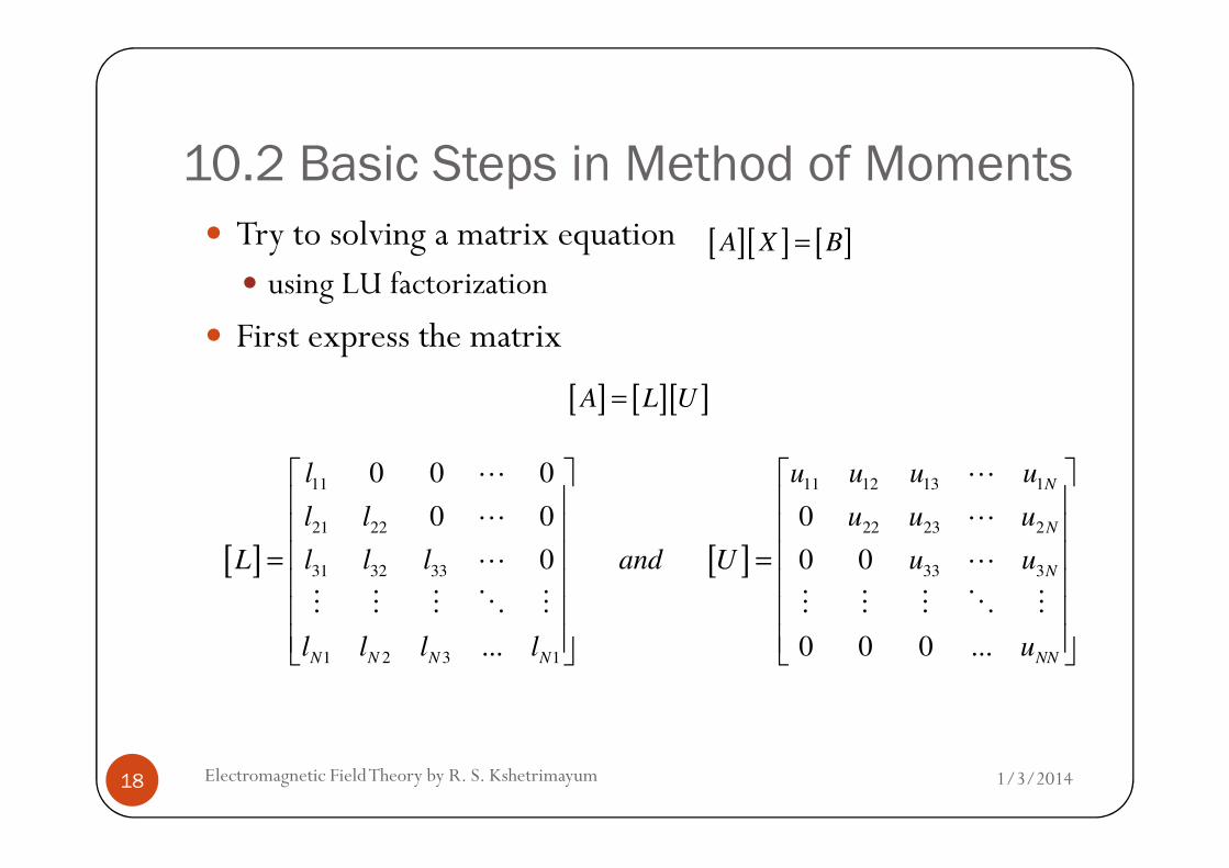
� Try to solving a matrix equation � using LU factorization
� First express the matrix
[ ] [ ][ ]A L U=
[ ][ ] [ ]A X B=
1/3/2014Electromagnetic Field Theory by R. S. Kshetrimayum18
[ ] [ ]
11 11 12 13 1
21 22 22 23 2
31 32 33 33 3
1 2 3 1
0 0 0
0 0 0
0 0 0
... 0 0 0 ...
N
N
N
N N N N NN
l u u u u
l l u u u
L l l l and U u u
l l l l u
= =
L L
L L
L L
M M M O M M M M O M

10.2 Basic Steps in Method of Moments
� through the forward substitution
[ ][ ][ ] [ ] [ ][ ] [ ]L U X B L Y B∴ = ⇒ =
11
1
1; , 1
i
i i ik k
by y b l y i
− = = − > ∑
1/3/2014Electromagnetic Field Theory by R. S. Kshetrimayum19
� through the backward substitution
1
111
; , 1i i ik k
kii
y y b l y il l =
= = − >
∑
[ ][ ] [ ]U X Y=
1
1; ,
NN
N i i ik k
k iNN ii
yx x y u x i N
u u = +
= = − <
∑

10.2 Basic Steps in Method of Moments
� This is more efficient than Gaussian elimination � since the RHS remain unchanged during the whole process
� The main issue here is to � find the lower and upper triangular matrices.
� MATLAB command for LU factorization of a matrix A is
1/3/2014Electromagnetic Field Theory by R. S. Kshetrimayum20
� MATLAB command for LU factorization of a matrix A is � [L U] = lu(A)
10.2 Basic Steps in Method of Moments
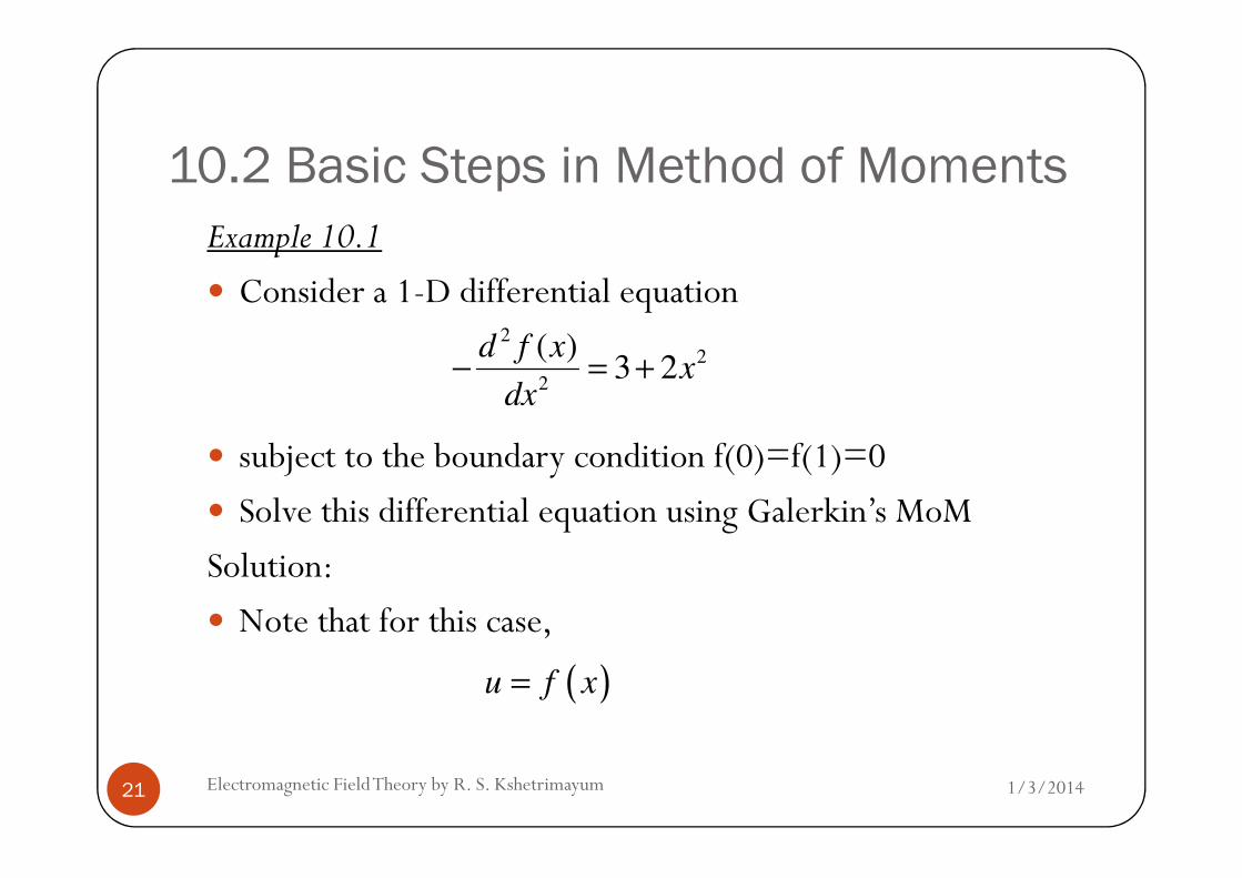
Example 10.1
� Consider a 1-D differential equation
subject to the boundary condition f(0)=f(1)=0
22
2
( )3 2
d f xx
dx− = +
1/3/2014Electromagnetic Field Theory by R. S. Kshetrimayum21
� subject to the boundary condition f(0)=f(1)=0
� Solve this differential equation using Galerkin’s MoM
Solution:
� Note that for this case,
( )u f x=

10.2 Basic Steps in Method of Moments
� According to the nature of the known function ,
it is natural to choose the basis function as
23 2k x= +
2
2
dL
dx= −
23 2k x= +
( ) nb x x=
1/3/2014Electromagnetic Field Theory by R. S. Kshetrimayum22
� it is natural to choose the basis function as
� However,
� the boundary condition f(1)=0 � can’t be satisfied with such a basis function
( ) n
nb x x=

10.2 Basic Steps in Method of Moments
� A suitable basis function for this differential equation � taking into account of this boundary condition is
� Assume N=2 (the total number of subsections on the
( ) 1; 1,2,...,n
nb x x x n N
+= − =
1/3/2014Electromagnetic Field Theory by R. S. Kshetrimayum23
� Assume N=2 (the total number of subsections on the interval [0,1])
� Approximation of the unknown function
( ) ( )2 3
1 1 2 2 1 2( ) ( ) ( )f x I b x I b x I x x I x x≅ + = − + −

10.2 Basic Steps in Method of Moments
� For Galerkin’s MoM, the weighting functions are
� Choosing a square [Z] matrix where M=N=2
( ) 1; 1,2,...,m
mw x x x m M
+= − =
1/3/2014Electromagnetic Field Theory by R. S. Kshetrimayum24
( ) ( ) ( )1 1
2
11 1 1 1 1
0 0
1, ( ) ( ) ( ) 2
3Z w L b w x L b x dx x x dx= = = − =∫ ∫
( ) ( ) ( )1 1
2
12 1 2 1 2
0 0
1, ( ) ( ) ( ) 6
2Z w L b w x L b x dx x x x dx= = = − =∫ ∫

10.2 Basic Steps in Method of Moments
( ) ( ) ( )1 1
3
21 2 1 2 1
0 0
1, ( ) ( ) ( ) 2
2Z w L b w x L b x dx x x dx= = = − =∫ ∫
( ) ( ) ( )1 1
3
22 2 2 2 2
0 0
4, ( ) ( ) ( ) 6
5Z w L b w x L b x dx x x x dx= = = − =∫ ∫
1/3/2014Electromagnetic Field Theory by R. S. Kshetrimayum25
( )1 1
2 2
1 1 1
0 0
3, ( ) ( ) 3 2 ( )
5V k w k x w x dx x x x dx= = = + − =∫ ∫
( )1 1
2 3
2 2 2
0 0
11, ( ) ( ) 3 2 ( )
12V k w k x w x dx x x x dx= = = + − =∫ ∫

10.2 Basic Steps in Method of Moments
� Therefore,
[ ][ ] [ ] 1
2
1 1 3
3 2 5
1 4 11
2 5 12
IZ I V
I
= ⇒ =
[ ] 1
13
10I
⇒ = =
1/3/2014Electromagnetic Field Theory by R. S. Kshetrimayum26
� The unknown function f(x)
[ ] 1
2
10
1
3
II
I
⇒ = =
( ) ( ) ( ) ( )2 3 2 3
1 2
13 1( )
10 3f x I x x I x x x x x x≅ − + − = − + −

10.2 Basic Steps in Method of Moments
� The above function satisfies the given boundary conditions � f(0)=f(1)=0
� The analytical solution for this differential equation is
2 45 3 1( )
3 2 6f x x x x= − −
1/3/2014Electromagnetic Field Theory by R. S. Kshetrimayum27
� Check whether the above solution using MoM is � different from the analytical solution obtained by direct integration (see Fig. 10.1)
3 2 6

10.2 Basic Steps in Method of Moments
1/3/2014Electromagnetic Field Theory by R. S. Kshetrimayum28
� Fig. 10.1 Comparison of exact solution (analytical) and approximate solution (MoM) of Example 10.1

10.3 Introductory examples from electrostatics
� In electrostatics, the problem of finding the potential � due to a given charge distribution is often considered
� In practical scenario, it is very difficult to � specify a charge distribution
� We usually connect a conductor to a voltage source
1/3/2014Electromagnetic Field Theory by R. S. Kshetrimayum29
� and thus the voltage on the conductor is specified
� We will consider MoM� to solve for the electric charge distribution
� when an electric potential is specified � Examples 2 and 3 discuss about calculation of inverse using LU decomposition and SVD
10.3 Introductory examples from electrostatics
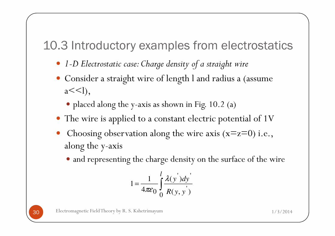
� 1-D Electrostatic case: Charge density of a straight wire
� Consider a straight wire of length l and radius a (assume a<<l), � placed along the y-axis as shown in Fig. 10.2 (a)
� The wire is applied to a constant electric potential of 1V
1/3/2014Electromagnetic Field Theory by R. S. Kshetrimayum30
� The wire is applied to a constant electric potential of 1V
� Choosing observation along the wire axis (x=z=0) i.e., along the y-axis � and representing the charge density on the surface of the wire
∫=
l
yyR
dyy
0'
''
0 ),(
)(
4
11
λ
πε

∆
1/3/2014Electromagnetic Field Theory by R. S. Kshetrimayum31
10.3 Introductory examples from electrostatics
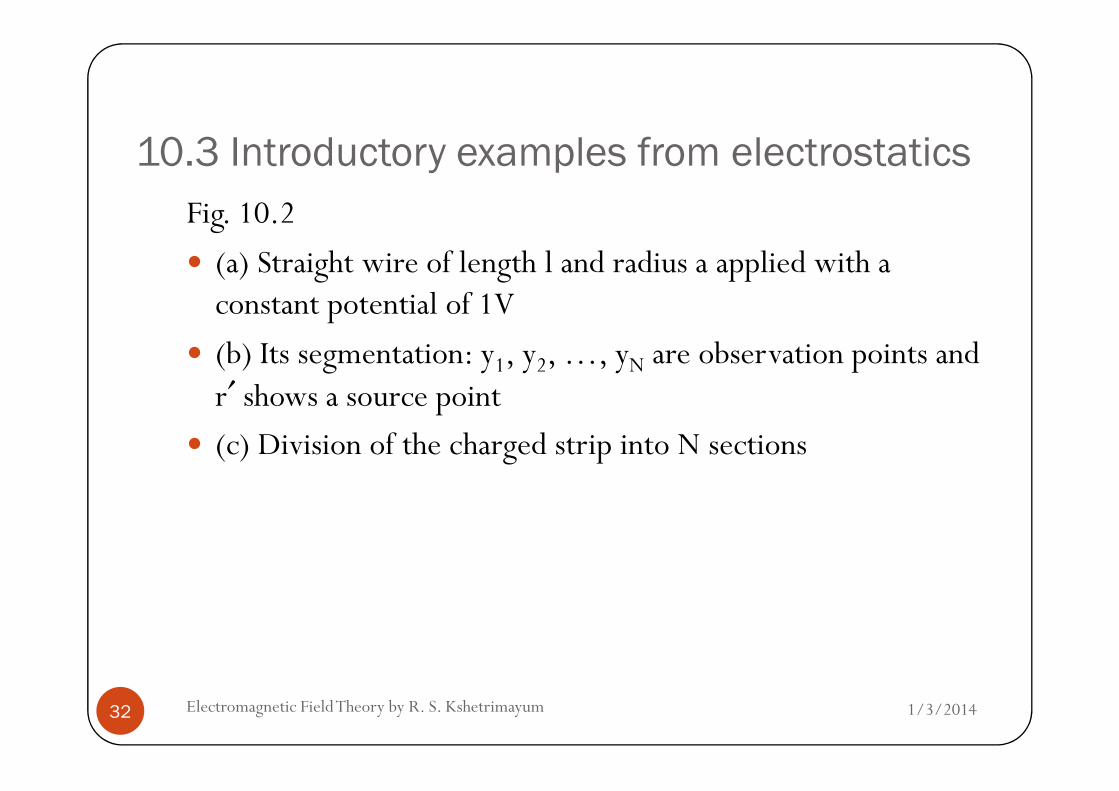
Fig. 10.2
� (a) Straight wire of length l and radius a applied with a constant potential of 1V
� (b) Its segmentation: y1, y2, …, yN are observation points and r′ shows a source point
1/3/2014Electromagnetic Field Theory by R. S. Kshetrimayum32
r′ shows a source point
� (c) Division of the charged strip into N sections

10.3 Introductory examples from electrostatics
� where
� It is necessary to solve the integral equation
to find the unknown function λ(y′)
' ' ' 2 ' 2 ' 2 ' 2 2
0( , ) ( , ) ( ) ( ) ( ) ( ) ( )
x zR y y R r r y y x z y y a
= == = − + + = − +
r r
1/3/2014Electromagnetic Field Theory by R. S. Kshetrimayum33
� to find the unknown function λ(y′)
� The solution may be obtained numerically by � reducing the integral equation into a series of linear algebraic equations
� that may be solved by conventional matrix techniques

10.3 Introductory examples from electrostatics
� (a) Approximate the unknown charge density λ(y′) � by an expansion of N known basis functions with unknown coefficients
∑=
=N
n
nn ybIy
1
'' )()(λ
1/3/2014Electromagnetic Field Theory by R. S. Kshetrimayum34
� Integral equation after substituting this is
∫∫ ∑∑
=
= ==
ln
l N
n
n
N
n
nn
yyR
dyybI
yyR
dyybI
0'
''
0 1'
'
1
'
0),(
)(
),(
)(
4πε

10.3 Introductory examples from electrostatics
� Now we have divided the wire into N uniform segments each of length ∆ as shown in Fig. 10.2 (b)
� We will choose our basis functions as pulse functions
( )
∆≤≤∆−
=otherwise
nynforybn
'' )1(
0
1
1/3/2014Electromagnetic Field Theory by R. S. Kshetrimayum35
b) Applying the testing or weighting functions
� Let us apply the testing functions as delta functions for point matching
otherwise0
( )my y ∂ −

10.3 Introductory examples from electrostatics
� Integration of any function with this delta function � will give us the function value at
� Replacing observation variable y by a fixed point such as ym, � results in an integrand that is solely a function of y′
� so the integral may be evaluated.
my y=
1/3/2014Electromagnetic Field Theory by R. S. Kshetrimayum36
� so the integral may be evaluated.
� It leads to an equation with N unknowns
∫ ∫ ∫∫∆
∆
∆
∆− ∆−
∆
+++++=
2
)1( )1('
''
'
''
'
''2
2
0'
''1
10),(
)(...
),(
)(...
),(
)(
),(
)(4
n
n
l
N m
NN
m
nn
mm yyR
dyybI
yyR
dyybI
yyR
dyybI
yyR
dyybIπε

10.3 Introductory examples from electrostatics
� Solution for these N unknown constants, � N linearly independent equations are required
� N equations may be produced � by choosing an observation point y on the wire and
1/3/2014Electromagnetic Field Theory by R. S. Kshetrimayum37
� by choosing an observation point ym on the wire and
� at the center of each ∆ length element
� as shown in Fig. 10.2 (c)
� Result in an equation of the form of the previous equation � corresponding to each observation point

10.3 Introductory examples from electrostatics
� For N such observation points we have
∫ ∫ ∫∫∆
∆
∆
∆− ∆−
∆
+++++=
2
)1( )1('
1
''
'1
''
'1
''2
2
0'
1
''1
10),(
)(...
),(
)(...
),(
)(
),(
)(4
n
n
l
N
NN
nn
yyR
dyybI
yyR
dyybI
yyR
dyybI
yyR
dyybIπε
∫ ∫ ∫∫∆ ∆∆ 2 ''''''
2''
1 )()()()(n l
Nn dyybdyybdyybdyyb
1/3/2014Electromagnetic Field Theory by R. S. Kshetrimayum38
∫ ∫ ∫∫∆
∆
∆
∆− ∆−
∆
+++++=
2
)1( )1('
2
''
'2
''
'2
''2
2
0'
2
''1
10),(
)(...
),(
)(...
),(
)(
),(
)(4
n
n
l
N
NN
nn
yyR
dyybI
yyR
dyybI
yyR
dyybI
yyR
dyybIπε
∫ ∫ ∫∫∆
∆
∆
∆− ∆−
∆
+++++=
2
)1( )1('
''
'
''
'
''2
2
0'
''1
10),(
)(...
),(
)(...
),(
)(
),(
)(4
n
n
l
N N
NN
N
nn
NN yyR
dyybI
yyR
dyybI
yyR
dyybI
yyR
dyybIπε
10.3 Introductory examples from electrostatics
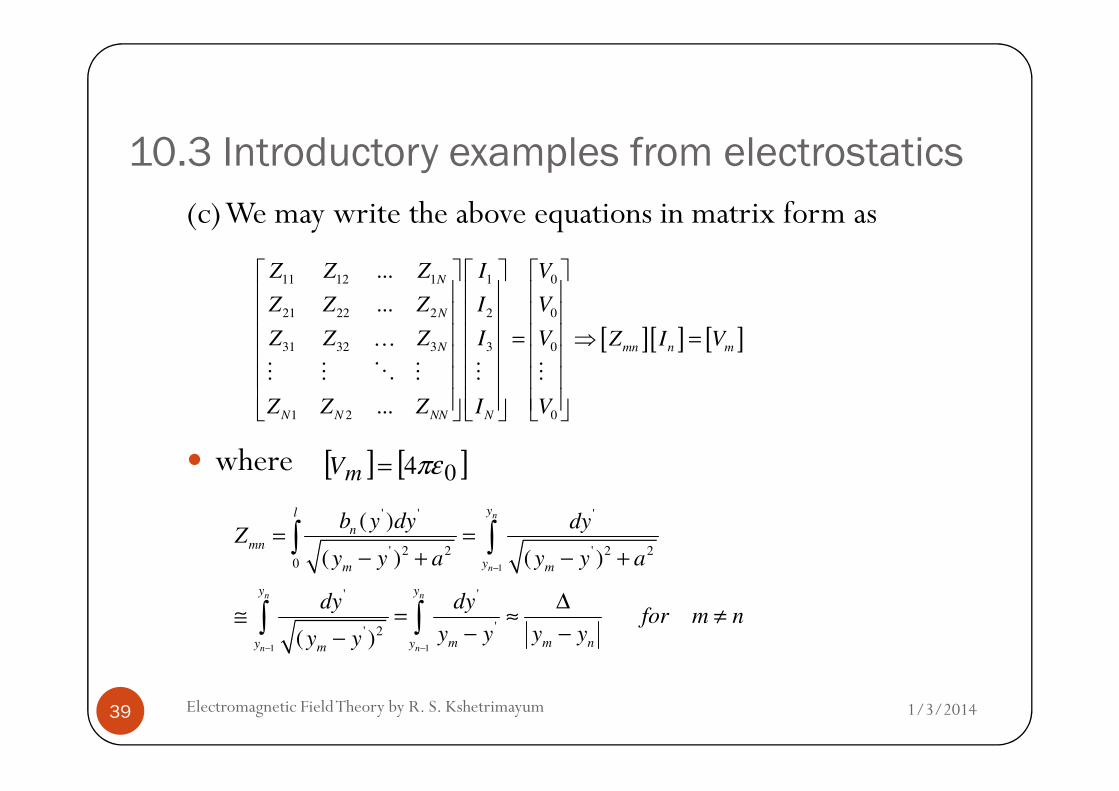
(c) We may write the above equations in matrix form as
[ ][ ] [ ]
11 12 1 1 0
21 22 2 2 0
31 32 3 3 0
...
...
...
N
N
N mn n m
Z Z Z I V
Z Z Z I V
Z Z Z I V Z I V
Z Z Z I V
= ⇒ =
K
OM M M M M
1/3/2014Electromagnetic Field Theory by R. S. Kshetrimayum39
� where
1 2 0...N N NN NZ Z Z I V
[ ] [ ]04πε=mV
1
1 1
' ' '
' 2 2 ' 2 20
' '
'' 2
( )
( ) ( )
( )
n
n
n n
n n
yl
n
mn
ym m
y y
m m ny ym
b y dy dyZ
y y a y y a
dy dyfor m n
y y y yy y
−
− −
= =− + − +
∆≅ = ≈ ≠
− −−
∫ ∫
∫ ∫

10.3 Introductory examples from electrostatics
� Special care for calculating the Zmn for m=n case � since the expression for Zmn is infinite for this case
� Extraction of this singularity
� Substitute ' '
my y d dyξ ξ− = ⇒ = −
1/3/2014Electromagnetic Field Theory by R. S. Kshetrimayum40
( )0
2 2
2 2 2 200
log ( )( ) ( )
mn
d dZ a
a a
ξ ξξ ξ
ξ ξ
∆ ∆
∆
= − = = + ++ +
∫ ∫
2 2
lna
a
∆ + ∆ +=

10.3 Introductory examples from electrostatics
� Self or diagonal terms are the � most dominant elements in the [Z] matrix
� Note that linear geometry of this problem � yields a matrix that is symmetric toeplitz, i.e.,
1/3/2014Electromagnetic Field Theory by R. S. Kshetrimayum41
[ ]
11 12 1
12 11 1 1
1 1 1 11
...
...
. . . .
...
N
N
mn
N N
Z Z Z
Z Z ZZ
Z Z Z
−
−
=
10.3 Introductory examples from electrostatics
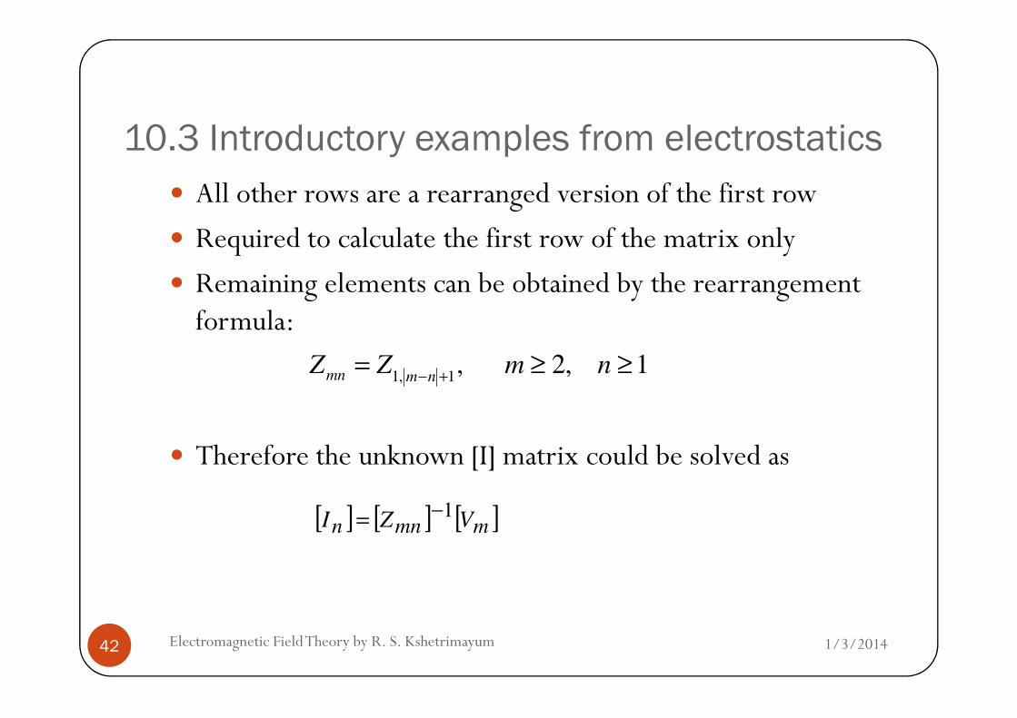
� All other rows are a rearranged version of the first row
� Required to calculate the first row of the matrix only
� Remaining elements can be obtained by the rearrangement formula:
, 2, 1Z Z m n= ≥ ≥
1/3/2014Electromagnetic Field Theory by R. S. Kshetrimayum42
� Therefore the unknown [I] matrix could be solved as
1, 1, 2, 1mn m n
Z Z m n− +
= ≥ ≥
[ ] [ ] [ ]mmnn VZI 1−=

1/3/2014Electromagnetic Field Theory by R. S. Kshetrimayum43
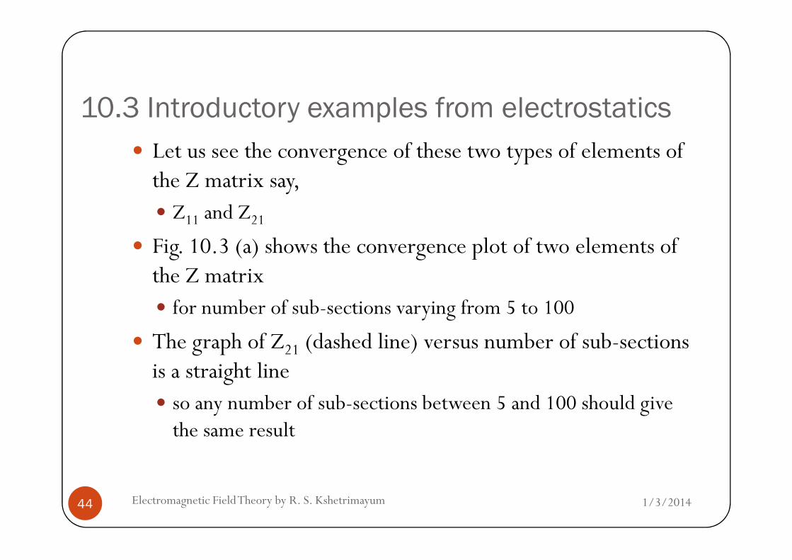
� Fig. 10.3 (a) Convergence plot of Z11 and Z21 (b) Plot of line charge density of the wire (MATLAB program provided in the book)
10.3 Introductory examples from electrostatics
� Let us see the convergence of these two types of elements of the Z matrix say, � Z11 and Z21
� Fig. 10.3 (a) shows the convergence plot of two elements of the Z matrix
1/3/2014Electromagnetic Field Theory by R. S. Kshetrimayum44
the Z matrix � for number of sub-sections varying from 5 to 100
� The graph of Z21 (dashed line) versus number of sub-sections is a straight line � so any number of sub-sections between 5 and 100 should give the same result

10.3 Introductory examples from electrostatics
� But the graph of Z11 versus number of sub-sections is � decreasing quite fast at the initial values of number of sub-sections and
� it is decreasing more slowly for larger values of number of sub-sections
1/3/2014Electromagnetic Field Theory by R. S. Kshetrimayum45
sections
� This shows that at � higher values of number of sub-sections,
� we will get a more convergent result
� Choose the maximum number of sub-sections and � plot the line charge density as depicted in the Fig. 10.3 (b)

10.3 Introductory examples from electrostatics
� See the condition number of the [Z] matrix in order to see � whether the [Z] matrix is well-behaved or not
� The condition number of [Z] matrix � (=7.1409) for maximum number of sub-sections is good
� No problem in taking the inverse
1/3/2014Electromagnetic Field Theory by R. S. Kshetrimayum46
� No problem in taking the inverse
� Fig. 10.3 (b) line charge density is � maximum at the two end points of the wire and
� minimum at the center of the wire
� 2-D Electrostatic case: Charge density of a square conducting plate discussed in the book

10.4 Some commonly used basis functions
� The weighted sum of basis functions is � used to represent the unknown function in MoM
� Choose a basis function that reasonably approximates � the unknown function over the given interval
� Basis functions commonly used in antenna or scattering
1/3/2014Electromagnetic Field Theory by R. S. Kshetrimayum47
� Basis functions commonly used in antenna or scattering problems are of two types: � entire domain functions and
� sub-domain functions

10.4 Some commonly used basis functions
10.4.1 Entire domain basis functions� The entire domain functions exist over the full domain -l/2<x<l/2� Some examples are:� Fourier (is well known)
−
=xn
xbn2
)1
(cos)(
1/3/2014Electromagnetic Field Theory by R. S. Kshetrimayum48
� Fourier (is well known)
� Chebyshev (will discuss briefly)
� Legendre (will discuss briefly)� where n=1,2,3,…,N.
=
lxbn )
2(cos)(
)2
()( 22l
xTxb nn −=
)2
()( 22l
xPxb nn −=

10.4 Some commonly used basis functions
� Chebyshev's differential equation
� where n is a real number
Solutions Chebyshev functions of degree n
( ) 01 2'''2 =+−− ynxyyx
1/3/2014Electromagnetic Field Theory by R. S. Kshetrimayum49
� Solutions Chebyshev functions of degree n
� n is a non-negative integer, i.e., n=0,1,2,3,…, � the Chebyshev functions are called Chebyshev polynomials denoted by Tn(x)

10.4 Some commonly used basis functions
� A Chebyshev polynomial at one point can be � expressed by neighboring Chebyshev polynomials at the same point
� whereT0(x)=1, T1(x)=x
( ) ( ) ( )xTxxTxT nnn 11 2 −+ −=
1/3/2014Electromagnetic Field Theory by R. S. Kshetrimayum50
� whereT0(x)=1, T1(x)=x
� Legendre's differential equation
� where n is a real number
( ) ( ) 0121 '''2 =++−− ynnxyyx

10.4 Some commonly used basis functions
� Solutions of this equation are called Legendre functions of degree n
� When n is a non-negative integer, i.e., n=0,1,2,3,…, � the Legendre functions are called Legendre polynomials denoted by Pn(x)
1/3/2014Electromagnetic Field Theory by R. S. Kshetrimayum51
by Pn(x)
� Legendre polynomial at one point can be � expressed by neighboring Legendre polynomials at the same point
� where P0(x)=1, P1(x)=x
( ) ( ) ( ) ( ) ( )xnPxxPnxPn nnn 11 121 −+ −+=+

10.4 Some commonly used basis functions
� Disadvantage: entire domain basis function may not be applicable of any general problem� Choose a particular basis function for a particular problem
� Crucial and only experts in the area could do it efficiently
� Developing a general purpose MoM based software,
1/3/2014Electromagnetic Field Theory by R. S. Kshetrimayum52
� Developing a general purpose MoM based software, � software for analyzing almost every problem in electromagnetics
� this is not feasible
� Sub-domain basis functions could achieve this purpose

10.4 Some commonly used basis functions
10.4.2 Sub-domain basis functions
� Sub-domain basis functions exist only on one of the N overlapping segments � into which the domain is divided
� Some examples are:
1/3/2014Electromagnetic Field Theory by R. S. Kshetrimayum53
� Some examples are:
� Piecewise constant function (pulse)
1 [ 1] [ ]( )
0n
x n x x nb x
otherwise
− < <=

10.4 Some commonly used basis functions
� Piecewise triangular function
[ 1] [ 1]( )
0
n
n
x xx n x x n
b x
otherwise
∆ − −− < < +
= ∆
1/3/2014Electromagnetic Field Theory by R. S. Kshetrimayum54
1
1
1
1
[ 1] [ ]
[ ] [ 1]
0
n
n n
n
n n
x xx n x x n
x x
x xx n x x n
x x
otherwise
−
−
+
+
−− < < −
−
= < < +−

10.4 Some commonly used basis functions
� Piecewise sinusoidal function ( ){ }( )
( ){ }( ){ }
{ }1
sin[ 1] [ 1]
( ) sin
0
sin[ 1] [ ]
sin
n
n
n
n n
k x xx n x x n
b x k
otherwise
k x xx n x x n
k x x −
∆ − − − < < +
= ∆
−− < <
−
1/3/2014Electromagnetic Field Theory by R. S. Kshetrimayum55
� where ∆=l/N, assuming equal subintervals but it is not mandatory and k is a constant
( ){ }( ){ }
1
1
sin[ ] [ 1]
sin
0
n
n n
k x xx n x x n
k x x
otherwise
+
−
−
= < < +−

10.4 Some commonly used basis functions
1/3/2014Electromagnetic Field Theory by R. S. Kshetrimayum56
� Fig. 10.5 Sub-domain basis functions (a) Piecewise constant function (b) Piecewise triangular function (c) Piecewise sinusoidal function

10.4 Some commonly used basis functions
� Since the derivative of the pulse function is impulsive
� we cannot employ it for MoM problems
o where the linear operator L consists of derivatives
� Piecewise triangular and sinusoidal functions
1/3/2014Electromagnetic Field Theory by R. S. Kshetrimayum57
� may be used for such kinds of problems
� Piecewise sinusoidal functions are generally used
� for analysis of wire antennas since
� they can approximate sinusoidal currents in the wire antennas

10.5 Wire Antennas and Scatterers
� For Piece-wise triangular and sinusoidal functions
� when we have N points in an interval
� we will have N-1 sub-sections and
� N-2 basis functions may be used
1/3/2014Electromagnetic Field Theory by R. S. Kshetrimayum58
10.5 Wire Antennas and Scatterers
� Consider application of MoM techniques
� to wire antennas and scatterers
10.5 Wire Antennas and Scatterers
� Antennas can be distinguished from scatterers� in terms of the location of the source
� If the source is on the wire� it is regarded as antenna
� When the wire is far from the source
1/3/2014Electromagnetic Field Theory by R. S. Kshetrimayum59
� When the wire is far from the source � it acts as scatterer
� For the wire objects (antenna or scatterer) � we require to know the current distribution accurately

10.5 Wire Antennas and Scatterers
� Integral equations are derived and � solved for this purpose
Wire antennas
� Feed voltage to an antenna is known � and the current distribution could be calculated
1/3/2014Electromagnetic Field Theory by R. S. Kshetrimayum60
� and the current distribution could be calculated
� other antenna parameters such as � impedance,
� radiation pattern, etc.
� can be calculated

10.5 Wire Antennas and Scatterers
Wire scatterers
� Wave impinges upon surface of a wire scatterer� it induces current density
� which in turn is used to generate the scattered fields
� We will consider
1/3/2014Electromagnetic Field Theory by R. S. Kshetrimayum61
� We will consider
� how to find the current distribution on a � thin wire or
� cylindrical antenna
� using the MoM

10.5 Wire Antennas and Scatterers
10.5.1 Electric field integral equation (EFIE)
� On perfect electric conductor like metal� the total tangential electric field is zero
� Centrally excited cylindrical antenna (Fig. 10.6)
� have two kinds of electric fields viz.,
1/3/2014Electromagnetic Field Theory by R. S. Kshetrimayum62
� have two kinds of electric fields viz., � incident and
� scattered electric fields
t
tan tan tan tan tan0 0ot inc scat inc scatE E E E E= ⇒ + = ⇒ = −r r r r r

2∆
1/3/2014Electromagnetic Field Theory by R. S. Kshetrimayum63
� Fig. 10.6 A thin wire antenna of length L, radius a (a<<L) and feed gap 2∆

10.5 Wire Antennas and Scatterers� where the is the source or impressed field and
� can be computed from the
� current density induced on the cylindrical wire antenna due to the � incident or
� impressed field
incEr
scatEr
1/3/2014Electromagnetic Field Theory by R. S. Kshetrimayum64
� impressed field
10.5.2 Hallen’s and Pocklington's Integro-differential equation
� Let us consider a perfectly conducting wire of � length L and
� radius a such that a<<L and λ, the wavelength corresponding to the operating frequency

10.5 Wire Antennas and Scatterers
� Consider the wire to be a hollow metal tube � open at both ends
� Let us assume that an incident wave � impinges on the surface of a wire
� When the wire is an antenna
( )incE rr r
1/3/2014Electromagnetic Field Theory by R. S. Kshetrimayum65
� When the wire is an antenna� the incident field is produced by the feed at the gap (see Fig. 10.6)
� The impressed field is required � to be known on the surface of the wire
inc
zE

10.5 Wire Antennas and Scatterers
� Simplest excitation� delta-gap excitation
� For delta gap excitation (assumption) � excitation voltage at the feed terminal is constant and
� zero elsewhere
1/3/2014Electromagnetic Field Theory by R. S. Kshetrimayum66
� zero elsewhere
� Implies incident field� constant over the feed gap and
� zero elsewhere

10.5 Wire Antennas and Scatterers� 2V0 (from + V0 to -V0) voltage source applied
� across the feed gap 2∆,
� Incident field on the wire antenna can be expressed as
0 ;V
z
< ∆r
1/3/2014Electromagnetic Field Theory by R. S. Kshetrimayum67
� Induced current density � due to the incident or impressed electric field
� produces the scattered electric field
0 ;
0;2
inc
z
z
EL
z
< ∆ ∆= ∆ < <
r
( )scatE rr r
10.5 Wire Antennas and Scatterers
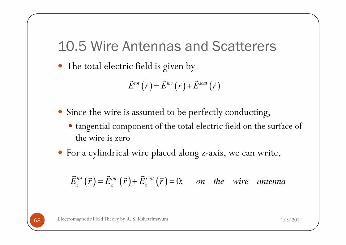
� The total electric field is given by
� Since the wire is assumed to be perfectly conducting,� tangential component of the total electric field on the surface of
( ) ( ) ( )tot inc scatE r E r E r= +r r rr r r
1/3/2014Electromagnetic Field Theory by R. S. Kshetrimayum68
� tangential component of the total electric field on the surface of the wire is zero
� For a cylindrical wire placed along z-axis, we can write,
( ) ( ) ( ) 0;tot inc scat
z z zE r E r E r on the wire antenna= + =r r rr r r

10.5 Wire Antennas and Scatterers
� that is,
� Find the electric field from the potential functions using
( ) ( )scat inc
z zE r E r= −r rr r
VAjE ∇−−=rr
ω
1/3/2014Electromagnetic Field Theory by R. S. Kshetrimayum69
� Lorentz Gauge condition,
VAjE ∇−−= ω
VjA 00εωµ−=•∇r
10.5 Wire Antennas and Scatterers
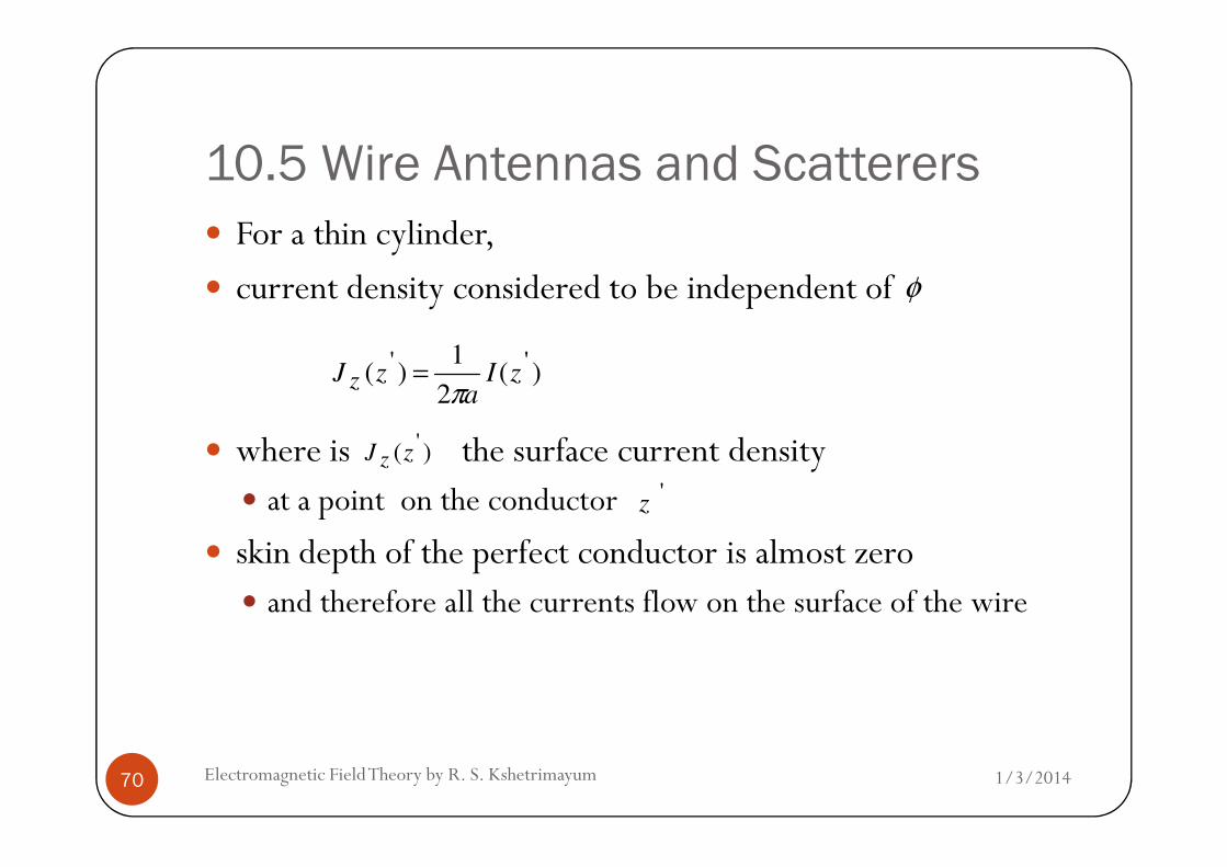
� For a thin cylinder,
� current density considered to be independent of
where is the surface current density
)(2
1)( ''
zIa
zJ zπ
=
φ
'
1/3/2014Electromagnetic Field Theory by R. S. Kshetrimayum70
� where is the surface current density � at a point on the conductor
� skin depth of the perfect conductor is almost zero � and therefore all the currents flow on the surface of the wire
)( 'zJ z
'z

10.5 Wire Antennas and Scatterers
� The current may be assumed to be
� a filamentary current located parallel to z-axis
� at a distance a (a is a very small number) as shown in the Fig. 10.7
� For the current flowing only in the z direction,
)('
zI
1/3/2014Electromagnetic Field Theory by R. S. Kshetrimayum71
� From Lorentz Gauge condition for time harmonic case,
z
VAjE zz
∂
∂−−= ω
2 2
0 0 0 02 2
0 0
1z z zA A AV Vj V j
z z z z j zωµ ε ωµ ε
ωµ ε
∂ ∂ ∂∂ ∂= − ⇒ = − ⇒ − =
∂ ∂ ∂ ∂ ∂
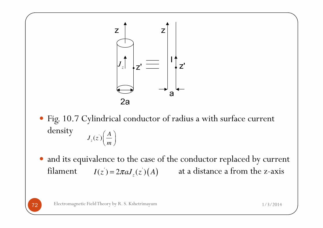
Fig. 10.7 Cylindrical conductor of radius a with surface current
zJ
1/3/2014Electromagnetic Field Theory by R. S. Kshetrimayum72
� Fig. 10.7 Cylindrical conductor of radius a with surface current density
� and its equivalence to the case of the conductor replaced by current filament at a distance a from the z-axis
'( )z
AJ z
m
( )' '( ) 2 ( )z
I z aJ z Aπ=

10.5 Wire Antennas and Scatterers
� Therefore,
� Magnetic vector potential can be expressed as
2 2 22 2
0 0 02 2 2
0 0 0 0 0 0
1 1 1z z zz z z z
A A AE j A A A
j z j z j zω ω µ ε β
ωµ ε ωµ ε ωµ ε
∂ ∂ ∂= − + = + = +
∂ ∂ ∂
1/3/2014Electromagnetic Field Theory by R. S. Kshetrimayum73
� Putting the Jz expression from (10.20), we have,
'0
4
0
dsr
eJA
rj
s
zzπ
µβ−
∫∫=
0/ 2 2 '
' '
0
/ 2 0
( )
2 4
L j r
z
L
I z eA ad dz
a r
π β
µ φπ π
−
−
= ∫ ∫

10.5 Wire Antennas and Scatterers
� where
� For ρ =a
( ) ( ) ( )2'2'2'zzyyxxr −+−+−=
0/ 2 2
' ' '1( ) ( )
L j re
A a I z d dz
π β
ρ µ φ−
= = ∫ ∫
1/3/2014Electromagnetic Field Theory by R. S. Kshetrimayum74
� where
' ' '
0
/ 2 0
1( ) ( )
2 4z
L
eA a I z d dz
rρ µ φ
π π−
= =
∫ ∫
( ) ( )2''
22
2sin4 zzaar −+
==
ϕρ

10.5 Wire Antennas and Scatterers
� Therefore, we can write
� where
'2/
2/
''0 ),()()( dzzzGzIaA
L
L
z ∫−
== µρ
02
' '1( , )
j re
G z z d
π β
φ−
= ∫
1/3/2014Electromagnetic Field Theory by R. S. Kshetrimayum75
� is the field at the observation point caused by a unit point source placed at
' '
0
1( , )
2 4
eG z z d
rφ
π π= ∫
),( 'rrGrr
'rr

10.5 Wire Antennas and Scatterers
� The field at by a source distribution � is the integral of over the range of occupied by the source
� The function G is called the Green's function
� We have,
rr
)( 'rJr
),()( ''rrGrJrrr '
rr
1/3/2014Electromagnetic Field Theory by R. S. Kshetrimayum76
� We have,
� and
+
∂
∂= z
zz A
z
A
jE
202
2
00
1β
µωε
0/ 2 2
' ' '
0
/ 2 0
1( ) ( )
2 4
L j r
z
L
eA a I z d dz
r
π β
ρ µ φπ π
−
−
= =
∫ ∫
10.5 Wire Antennas and Scatterers
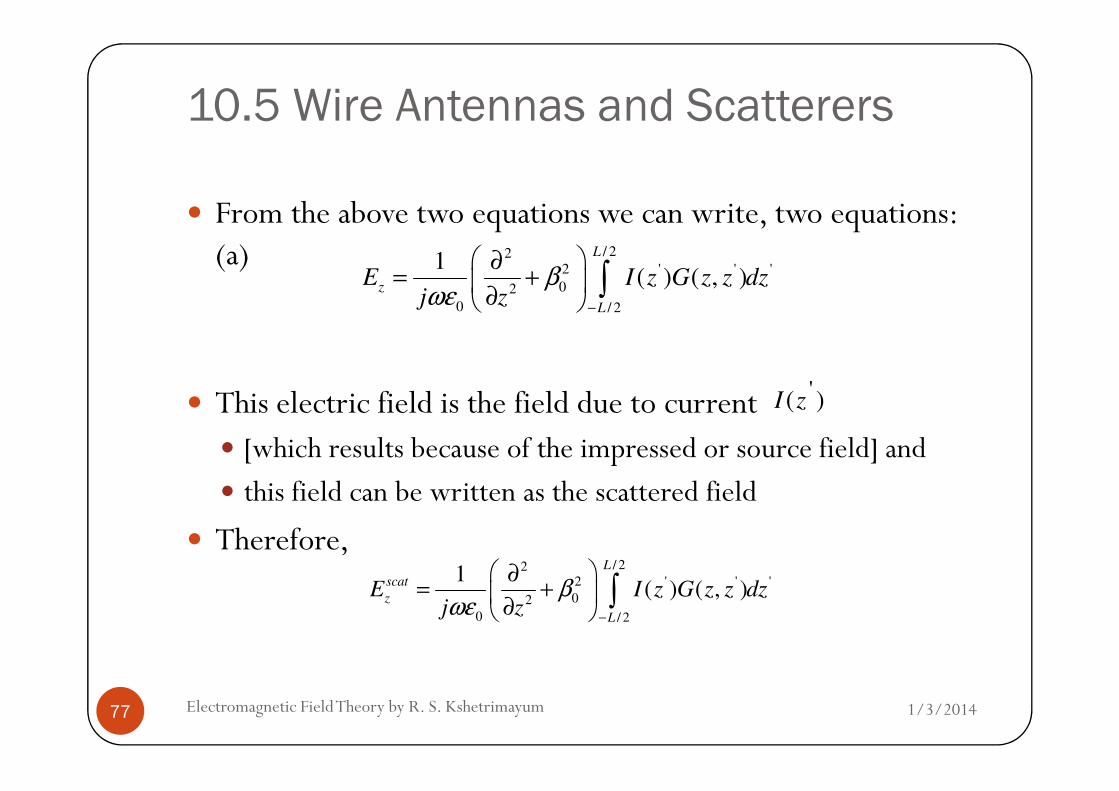
� From the above two equations we can write, two equations: (a)
� This electric field is the field due to current
/ 222 ' ' '
02
0 / 2
1( ) ( , )
L
z
L
E I z G z z dzj z
βωε
−
∂= +
∂ ∫
)( 'zI
1/3/2014Electromagnetic Field Theory by R. S. Kshetrimayum77
� This electric field is the field due to current � [which results because of the impressed or source field] and
� this field can be written as the scattered field
� Therefore,
)( 'zI
/ 222 ' ' '
02
0 / 2
1( ) ( , )
L
scat
z
L
E I z G z z dzj z
βωε
−
∂= +
∂ ∫
10.5 Wire Antennas and Scatterers
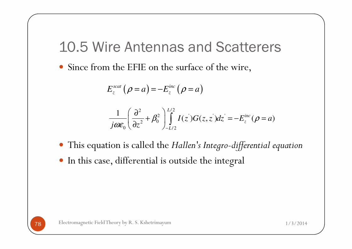
� Since from the EFIE on the surface of the wire,
( ) ( )scat inc
z zE a E aρ ρ= = − =
/ 222 ' ' '
02
1( ) ( , ) ( )
L
inc
zI z G z z dz E a
j zβ ρ
ωε
∂+ = − =
∂ ∫
1/3/2014Electromagnetic Field Theory by R. S. Kshetrimayum78
� This equation is called the Hallen's Integro-differential equation
� In this case, differential is outside the integral
2
0 / 2Lj zωε
−∂
∫
10.5 Wire Antennas and Scatterers
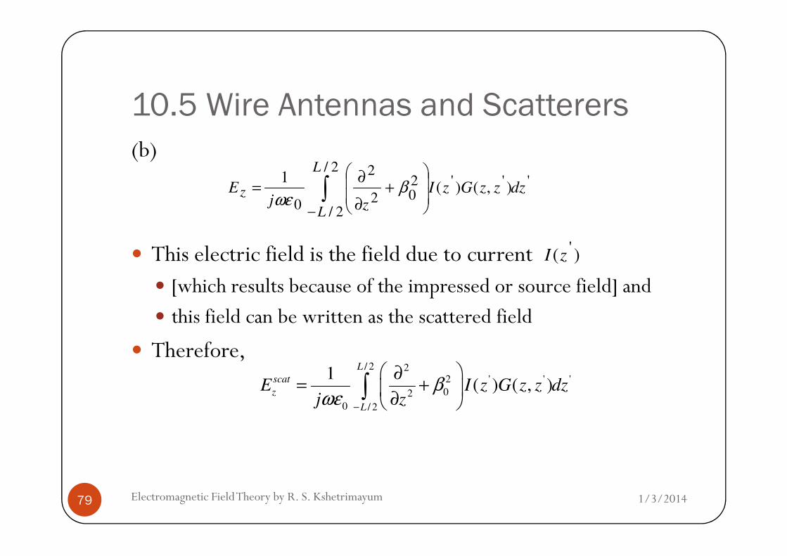
(b)
� This electric field is the field due to current � [which results because of the impressed or source field] and
'2/
2/
''202
2
0
),()(1
dzzzGzIzj
E
L
L
z ∫−
+
∂
∂= β
ωε
)( 'zI
1/3/2014Electromagnetic Field Theory by R. S. Kshetrimayum79
� [which results because of the impressed or source field] and
� this field can be written as the scattered field
� Therefore, / 2 2
2 ' ' '
02
0 / 2
1( ) ( , )
L
scat
z
L
E I z G z z dzj z
βωε
−
∂= +
∂ ∫

10.5 Wire Antennas and Scatterers
� Since from EFIE on the surface of the wire,
( ) ( )scat inc
z zE a E aρ ρ= = − =
/ 2 22 ' ' '
02
0 / 2
1( ) ( , ) ( )
L
inc
z
L
I z G z z dz E aj z
β ρωε
−
∂+ = − =
∂ ∫
1/3/2014Electromagnetic Field Theory by R. S. Kshetrimayum80
� This equation is the Pocklington's Integro-differential equation
� In this case, the differential has moved inside the integral
� Richmond has simplified the above equation as follows:
0 / 2Lj zωε
−∂

10.5 Wire Antennas and Scatterers
� (c) In cylindrical coordinates,
( )2 2
' ' 'r r r z z ρ ρ= − = − + −r rr r
( )' ' 2 2 ' 2 2 '2 2 cosa a a aρ ρ ρ ρ ρ ρ ρ ρ φ φ= ∴ − = + − • = + − −r r r r
Q
1/3/2014Electromagnetic Field Theory by R. S. Kshetrimayum81
� Problem under analysis has cylindrical symmetry and � observation for any values of won’t make any difference
� we may assume without loss of generality
� hence
( ) ( )2
' 2 2 ' '2 cosr r r a a z zρ ρ φ φ⇒ = − = + − − + −r r
φ
0φ =' 'φ φ φ− =

10.5 Wire Antennas and Scatterers
� where
and the inner integration
0/ 2 2'
' '
0
/ 2 0
( )
2 4
L j r
z
L
I z eA d dz
r
π β
µ φπ π
−
−
= ∫ ∫
( ) ( )2
2 2 ' '2 cosr a a z zρ ρ φ= + − + −
02
'j r
ed
π β
φ−
∫
1/3/2014Electromagnetic Field Theory by R. S. Kshetrimayum82
� and the inner integration � is also referred to as cylindrical wire kernel
� If we assume a<<λ and is very small, we have,
� Inner integrand is no more dependent on the variable
'
04
ed
rφ
π∫
( )2
2 'r z zρ≅ + −
'φ

10.5 Wire Antennas and Scatterers
� Therefore
� Also called as thin wire approximation � with the reduced kernel
0/ 2 '
'
0
/ 2
( )
4
L j r
z
L
I z eA dz
r
β
µπ
−
−
= ∫
1/3/2014Electromagnetic Field Theory by R. S. Kshetrimayum83
� with the reduced kernel
� For this case, we can write
( ) ( )0
',4
j re
G z z G rr
β
π
−
≅ =

10.5 Wire Antennas and Scatterers
� Now in the light of this simplification of the magnetic vector potential,
� we can simplify equation 10.29c (see example 10.4) as follows:
1/3/2014Electromagnetic Field Theory by R. S. Kshetrimayum84
� This form of the Pocklington’s integro-differential is more suitable for MoM formulation � since it does not involve any differentiation.
( )( ) ( )0
/ 22' 2 2 '
0 05
0 / 2
1( ) 1 2 3 ( )
4
L j r
inc
z z
L
eI z j r r a ar dz E a
j r
β
β β ρωε π
−
−
+ − + = − = ∫

10.5 Wire Antennas and Scatterers
10.5.3 MoM Formulation of Pocklington's Integro-differential equation
� Applying MoM formulation to above integral equation
� Divide the wire in to N segments
� Consider pulse basis function and
1/3/2014Electromagnetic Field Theory by R. S. Kshetrimayum85
� Consider pulse basis function and � express the current as a series expansion
� in the form of a staircase approximation as
where' '
1
( ) ( )N
n n
n
I z I b z=
=∑'
' 1( )
0
n
n
for zb z
otherwise
∆=
'
nz
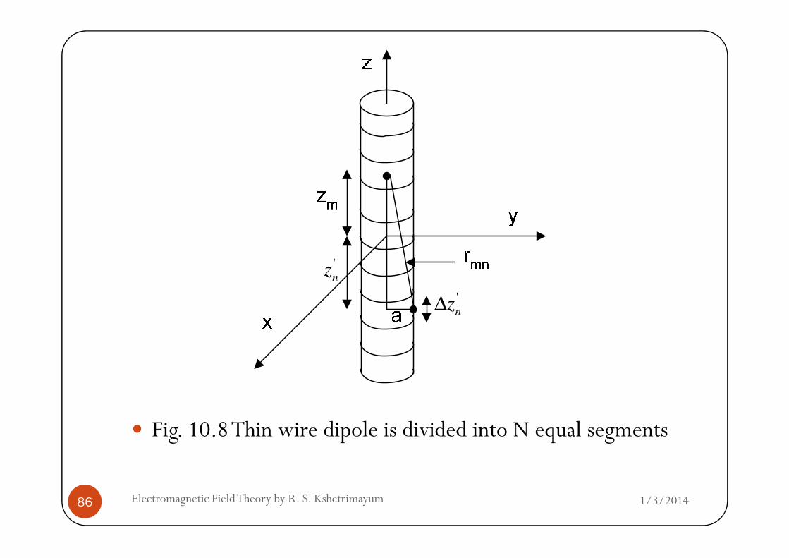
1/3/2014Electromagnetic Field Theory by R. S. Kshetrimayum86
� Fig. 10.8 Thin wire dipole is divided into N equal segments
'
nz∆
nz

10.5 Wire Antennas and Scatterers
� is the length of the nth segment, expressed as
( 1)2 2
L L L Ln z n
N N− + − < ≤ − +
'nz∆
/ 2
' ' '( ) ( , )
L
inc
zE I z F z z dz− = ∫
1/3/2014Electromagnetic Field Theory by R. S. Kshetrimayum87
� where
/ 2
( ) ( , )z
L
E I z F z z dz−
− = ∫
( )'202
2' ,
1),( zzG
zjzzF
+
∂
∂= β
ωε
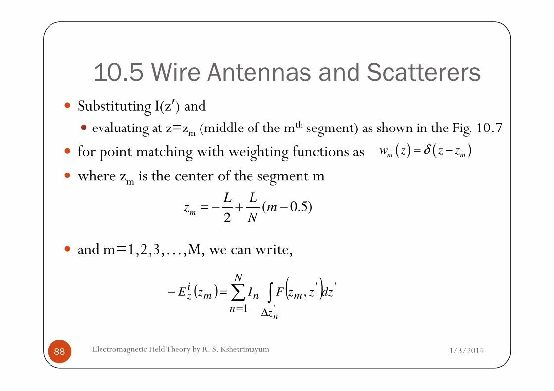
10.5 Wire Antennas and Scatterers� Substituting I(z′) and
� evaluating at z=zm (middle of the mth segment) as shown in the Fig. 10.7
� for point matching with weighting functions as
� where zm is the center of the segment m
( ) ( )m mw z z zδ= −
L L
1/3/2014Electromagnetic Field Theory by R. S. Kshetrimayum88
� and m=1,2,3,…,M, we can write,
( 0.5)2
m
L Lz m
N= − + −
( ) ( )∑ ∫= ∆
=−N
n z
mnmiz
n
dzzzFIzE
1
''
'
,

10.5 Wire Antennas and Scatterers
� To overcome the singularity � for the self term or diagonal elements of the [Z] matrix
� we have assumed that the source is on the surface of the wire � whereas the observation is the axis of the wire
� Using mid-point integration, we have,
1/3/2014Electromagnetic Field Theory by R. S. Kshetrimayum89
� Using mid-point integration, we have,
� where ( ) ( )∫∆
∆≅=
'
'''' ,,
nz
nnmmmn zzzFdzzzFF
( ) ∑=
=−N
n
mnnmiz FIzE
1
10.5 Wire Antennas and Scatterers
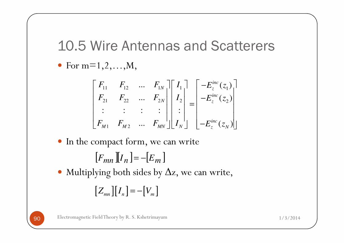
� For m=1,2,…,M,
11 12 1 1 1
21 22 2 2 2
... ( )
... ( )
: : : : :
... ( )
incN z
inc
N z
inc
F F F I E z
F F F I E z
F F F I E z
−
− = −
1/3/2014Electromagnetic Field Theory by R. S. Kshetrimayum90
� In the compact form, we can write
� Multiplying both sides by ∆z, we can write,
1 2 ... ( )incM M MN N z N
F F F I E z −
[ ][ ] [ ]mnmn EIF −=
[ ][ ] [ ]mn n mZ I V= −

10.5 Wire Antennas and Scatterers
� [In] can be computed by matrix inversion � Can find the approximate current distribution on the antenna
� Other important antenna parameters are � input impedance of the antenna and
� the total radiated fields
1/3/2014Electromagnetic Field Theory by R. S. Kshetrimayum91
� the total radiated fields
� which can be obtained as:
( ) ( ) ( ) ( )0
0
2
/ 2 2' 2 '
021/ 2
2
1( )
4
input
N
L j rNtot inc scat inc
n n
nL
VZ
I
eE r E r E r E r I b z dz
j z r
β
βωε π
−
=−
=
∂= + = + +
∂ ∑∫
r r r rr r r r

10.5 Wire Antennas and Scatterers
Example 10.5
� Consider a short dipole (thin wire antenna) of length 0.3λand radius 0.01λ.
� Find the current distribution on the short dipole and input impedance using MoM.
1/3/2014Electromagnetic Field Theory by R. S. Kshetrimayum92
impedance using MoM.
� Assume frequency of operation of the antenna is at 1 MHz.
� Choose the number of discretizations on the thin wire as three segments only.

10.5 Wire Antennas and Scatterers
� For three segments discretization ( ) on the thin wire antenna
� the MoM matrix equation will be
0.1z λ∆ =
11 12 13 1 1Z Z Z I V
Z Z Z I V
= −
1/3/2014Electromagnetic Field Theory by R. S. Kshetrimayum93
21 22 23 2 2
31 32 33 3 3
11 12 13 1 1
21 22 23 2 2
31 32 33 3 3
Z Z Z I V
Z Z Z I V
F F F I E
z F F F I z E
F F F I E
= −
⇒ ∆ = −∆

10.5 Wire Antennas and Scatterers
� where
Simplifying the above expression of the Z (see book)
( ) ( ) ( )022 2
0 0
5
0
1 2 3
4
mnj r
mn mn mn
mn mn
mn
e j r r a ar zZ F z
j r
β β β
ωε π
− + − + ∆ = ∆ =
1/3/2014Electromagnetic Field Theory by R. S. Kshetrimayum94
� Simplifying the above expression of the Zmn (see book)
2 2
0
3
2
1 2 2 3 2 cos 2 sin 2
8
mn mn mn
mn
mn
mn
r r rz a ajZ j j
rZ
r
π π π πλ λ λ λ λ
π λλ
∆ − + − + − =
10.5 Wire Antennas and Scatterers
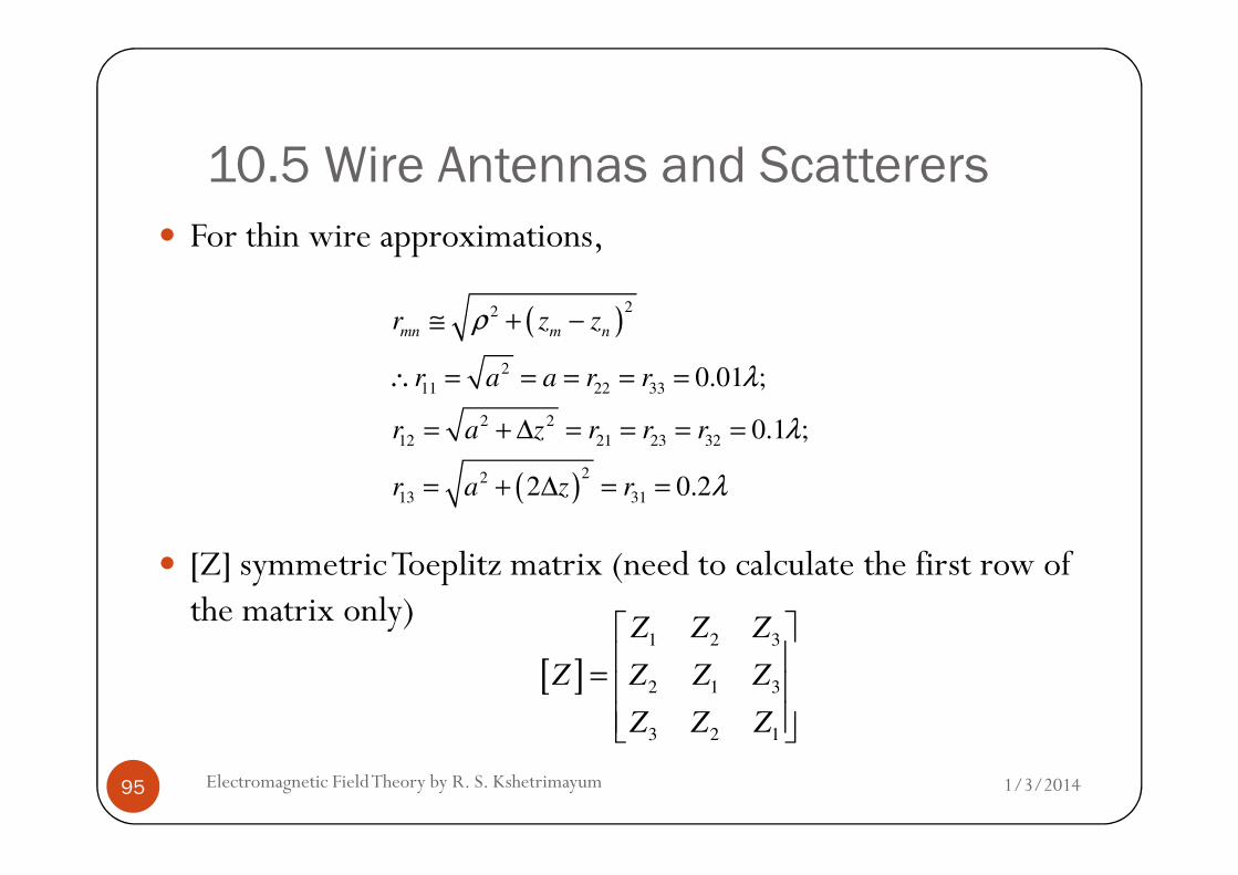
� For thin wire approximations,
( )22
2
11 22 33
2 2
12 21 23 32
0.01 ;
0.1 ;
mn m nr z z
r a a r r
r a z r r r
ρ
λ
λ
≅ + −
∴ = = = = =
= + ∆ = = = =
1/3/2014Electromagnetic Field Theory by R. S. Kshetrimayum95
� [Z] symmetric Toeplitz matrix (need to calculate the first row of the matrix only)
( )
12 21 23 32
22
13 31
0.1 ;
2 0.2
r a z r r r
r a z r
λ
λ
= + ∆ = = = =
= + ∆ = =
[ ]1 2 3
2 1 3
3 2 1
Z Z Z
Z Z Z Z
Z Z Z
=

10.5 Wire Antennas and Scatterers
� About the [V] matrix, for delta gap excitation,
since a voltage 1V exists at the feed gap only
[ ]0
1
0
V
= −
1/3/2014Electromagnetic Field Theory by R. S. Kshetrimayum96
� since a voltage 1V exists at the feed gap only
� Solve the [I] matrix and get the current distribution
� and the input impedance can be calculated as
0
2
2
2 1input
N
VZ
I I= =
10.6 Software language for implementation
of electromagnetics codes
� Choice of software languages for implementing electromagneticscode
� FORTRAN language complex numbers are a built-in datatype
� Many computational electromagnetics programmer prefer
1/3/2014Electromagnetic Field Theory by R. S. Kshetrimayum97
� Many computational electromagnetics programmer prefer � to use FORTRAN language
� for implementing their algorithms
� Earlier versions of FORTRAN were a functional language

10.6 Software language for implementation
of electromagnetics codes
� New versions of FORTRAN are object-oriented languages
� C++, another object-oriented language, � is also widely used for many numerical methods
� FORTRAN and C++ are efficient in implementation
1/3/2014Electromagnetic Field Theory by R. S. Kshetrimayum98
� FORTRAN and C++ are efficient in implementation � since the computational time is less
� MATLAB is also convenient environments since � it accepts complex numbers,
� graphics are very easy to create and
� many in-built functions are readily available for use

10.6 Software language for implementation
of electromagnetics codes
� MATLAB any additional “for” loop in the program, � the time it takes to run the program increases drastically
� Good to consider the advantages and disadvantages � for employment of any software language
1/3/2014Electromagnetic Field Theory by R. S. Kshetrimayum99
� for employment of any software language
� For instance, � drawing graphics in C is somewhat involved,
� but MATLAB is convenient for such things.
� program written in C runs faster than MATLAB and so on

10.6 Software language for implementation
of electromagnetics codes
� Computational electromagnetics is a topic � which you can learn only by doing
� Some simulation exercises are given at the end of the chapter,
� you should always write down a � MATLAB or
1/3/2014Electromagnetic Field Theory by R. S. Kshetrimayum100
� MATLAB or
� any other software language program
� in which you are comfortable and
� see those results

10.7 Summary
� Summarize the three steps involved in MoM:
(a) Derivation of appropriate integral equations
(b) Conversion or discretization of the integral equation into
� a matrix equation using � basis or expansion functions and
1/3/2014Electromagnetic Field Theory by R. S. Kshetrimayum101
� basis or expansion functions and
� weighting or testing functions
� as well as evaluation of the matrix elements
(c) Solving the matrix equation and
� obtaining the desired parameters