10.1 QUALITATIVE AND QUANTITATIVE COMPARISONS OF A BASE-STATE SUBSTITUTION

SIMULATION WITH DUAL-DOPPLER OBSERVATIONS OF THE 29 MAY 2012 KINGFISHER SUPERCELL

Casey E. Davenport*

University of North Carolina at Charlotte

M.I. Biggerstaff

School of Meteorology, University of Oklahoma

C.L. Ziegler

National Severe Storms Laboratory

1. MOTIVATION

A common approach to understanding the fundamental

processes of deep, moist convection has been to utilize

idealized numerical simulations. These simulations often

employ horizontally- and temporally-homogeneous

base-state conditions to isolate the key processes at

work, despite knowledge that heterogeneity is inherent

in many convective storm environments (e.g., Brooks et

al. 1996; Weckwerth et al. 1996; Markowski and

Richardson 2007). Much of what we understand about

convective storm dynamics arose from idealized

simulations that did not include horizontal or temporal

variability in the base-state environment (e.g., Klemp

1987). Accounting for environmental heterogeneity in an

idealized setting has largely been avoided because of

numerous complicating factors that can prevent a clean

separation of cause and effect in experimental results.

However, it is unknown how the fundamental processes

governing severe convection are influenced by changes

in the surrounding environment; there is evidence that

such processes can be significantly altered (e.g.,

Davenport and Parker 2015).

Base-state substitution (BSS; Letkewicz et al. 2013) is

an idealized modeling method that was designed

incorporate the effects of heterogeneity (i.e., changing

the base-state) without the complexities of introducing

spatial variability. Essentially, BSS approximates the

temporal tendencies in temperature, moisture, and wind

actually experienced by a storm as it encounters a

changing environment. In other words, a new proximity

sounding is imposed at a desired rate (see Letkewicz et

al. 2013, their Fig. 1). A schematic of the procedure for

BSS is shown in Fig. 1 and described in detail in

Letkewicz et al. (2013). Briefly, after a certain amount of

model run time, BSS separates out the storm-induced

perturbations of temperature, moisture, and wind from

the original base-state, and then replaces the original

* Corresponding author address: Casey E. Davenport,

University of North Carolina at Charlotte, Department of Geography and Earth Sciences, Charlotte, NC 28223; email: Casey.Davenport@uncc.edu

horizontally-homogeneous background environment

with a new horizontally-homogeneous environment; this

is completed at a prescribed temporal interval defined

by the model user. This approach permits the user to

independently modify temperature, moisture, or wind

profiles as desired, which provides a significant amount

of control over changes to the environment and

consequently allows the user to more readily identify

cause and effect in their experiments.

The primary assumption of BSS is that the integrated

effect of a storm moving across an environmental

gradient over time is larger than the instantaneous effect

of local storm-scale gradients. This assumption is

central not only to BSS, but to all idealized models with

horizontally-homogeneous environments employing a

representative proximity sounding to the entire domain.

The key question is whether this assumption is valid.

Will a BSS simulation, employing only temporal

variability, produce a realistic storm evolution? To what

extent is employing BSS more realistic than not

changing the environment at all? To address these

questions, idealized simulations with and without BSS

will be qualitatively and quantitatively compared to

observations of an isolated supercell thunderstorm.

2. OBSERVATIONS

The Kingfisher supercell thunderstorm, observed on 29

May 2012 during the Deep Convective Clouds and

Chemistry field program (DC3; Barth et al. 2015), was

chosen due to the availability of extensive observations

of the storm as the near-inflow environment evolved.

Three soundings (one pre-convective, two near-inflow)

Figure 1: Schematic of the procedure followed for base-

state substation. See Letkewicz et al. (2013) for more

details.

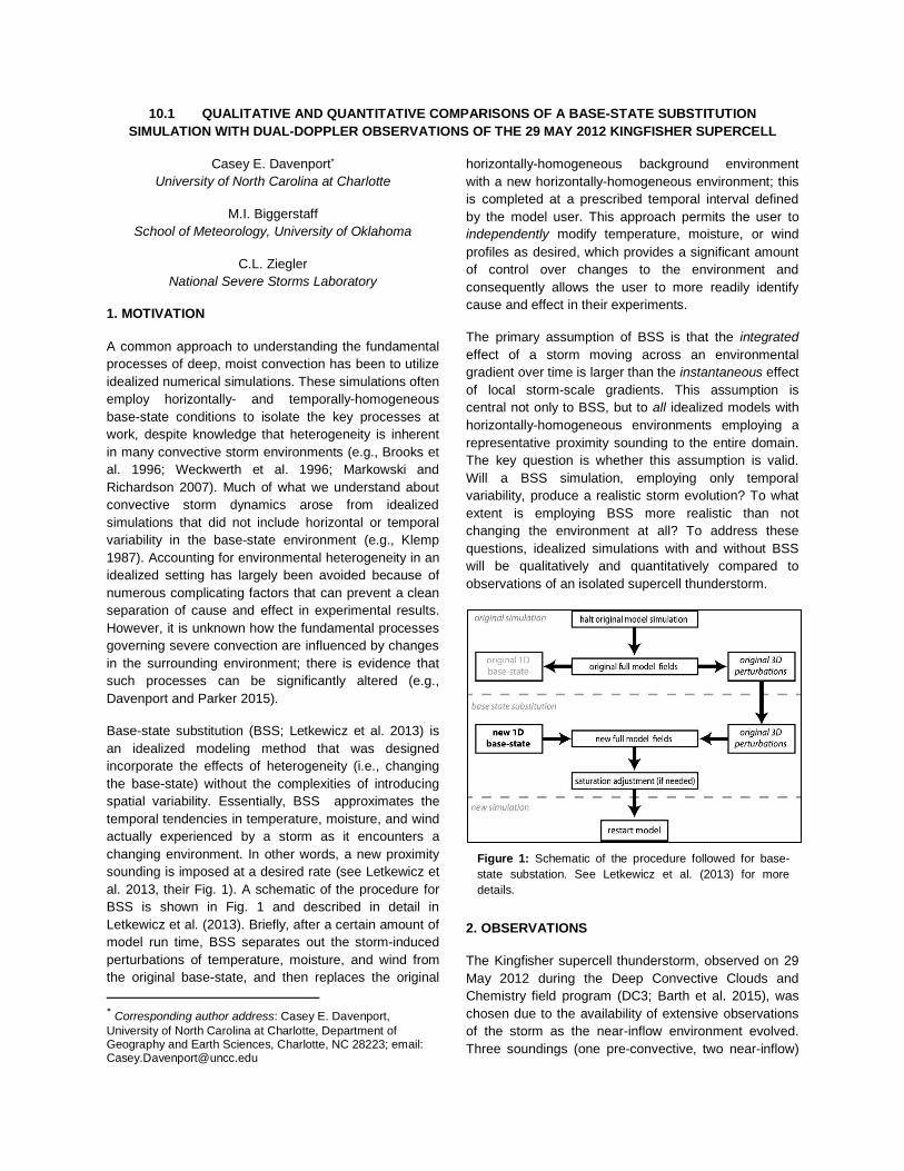
were launched over the lifetime of the storm, at 2029,

2255, and 0020 UTC, capturing notable modifications to

thermodynamic and kinematic profiles (Fig. 2; Table 1).

Overall, CAPE increased over time, CIN remained about

the same, but both 0-3 km SRH and BRN shear

significantly increased. The combination of these

environmental changes would support a more intense

rotating storm, which was indeed what was observed

(Fig. 3).

Multiple-Doppler data was collected between 2251 and

0000 UTC, providing key observations of storm

structure over an extended period of time, within which

the surrounding environment underwent significant

changes. Three mobile radars collected coordinated

scans of the Kingfisher storm: the two SMART-Rs

(Biggerstaff et al. 2005) and the NOXP radar (Burgess

et al. 2010). Time synced radar volumes were collected

every three minutes by all three radars, however the

storm was never located in the triple-Doppler region.

Wind retrieval was achieved using the variational

method described in Potvin et al. (2012). A nearby

environmental sounding provided the background field

for the analysis, which was then blended with the storm

using a low-pass filter. Each radar volume was

interpolated to a 90 x 60 x 17.5 km Cartesian grid using

natural neighbor interpolation (Ledoux and Gold 2005).

The horizontal and vertical grid spacing was 500 m.

3. MODEL EXPERIMENTS

The idealized numerical model CM1 (Bryan and Fritsch

2002), release 18, was utilized for the modeling

component of this study. The domain was 300 x 400 x

21 km, with a horizontal grid spacing of 500 m (same as

the observations) and a stretched vertical grid (100 m

near the model surface to 500 m aloft). Convection was

initiated using moist convergence (relative humidity

Figure 2: Skew-T log-p diagrams of observed inflow soundings from DC3 experiment on 29-30 May 2012.

Parameter 2029 UTC 2255 UTC 0020 UTC

CAPE (J/kg) 2516 2599 3155

CIN (J/kg) -29 -37 -18

0-3 km SRH (m2/s2)

185 271 466

BRN Shear (m/s)

76 93 140

initially set at 95% within the zone of convergence;

Loftus et al. 2008) over the first 30 min of the simulation.

Microphysics were governed by the National Severe

Storm Laboratory’s double moment variable graupel and

hail density scheme (Mansell et al. 2010).

The observed soundings were utilized to describe the

horizontally-homogeneous base-state environment in

the model and were incorporated into the simulations

via the BSS technique. Note that in this study, the BSS

approach has been updated to occur every time step

before the model is integrated forward (hereafter

“continuous BSS”); no model restarts are needed. In

other words, a tendency is applied to base-state

variables based on the differences between the input

soundings. The perturbations of temperature, moisture,

and wind are still retained as before.

Convection was observed to initiate around 2130 UTC

on 29 May; to approximate this environment in the

model, a linear interpolation was performed between the

2029 UTC and 2255 UTC profiles. Slight moistening

was required (5% RH in the lowest 4 km) in order to

achieve long-lived convection in the model. This slightly

moistened environment thus represented the original

base-state in the model; the control simulation

maintained this background environment for the entirety

of the simulation (5 hours). In the BSS simulation, the

base-state temperature, moisture, and wind profiles

were continuously modified to the 2255 and 0020 UTC

profiles once an isolated supercell developed, starting at

135 min into the simulation. Note that to maintain the

same observed change in moisture, the 2255 and 0020

UTC profiles were also slightly moistened; utilizing these

slightly modified profiles did not impact the results.

3. QUALITATIVE COMPARISONS

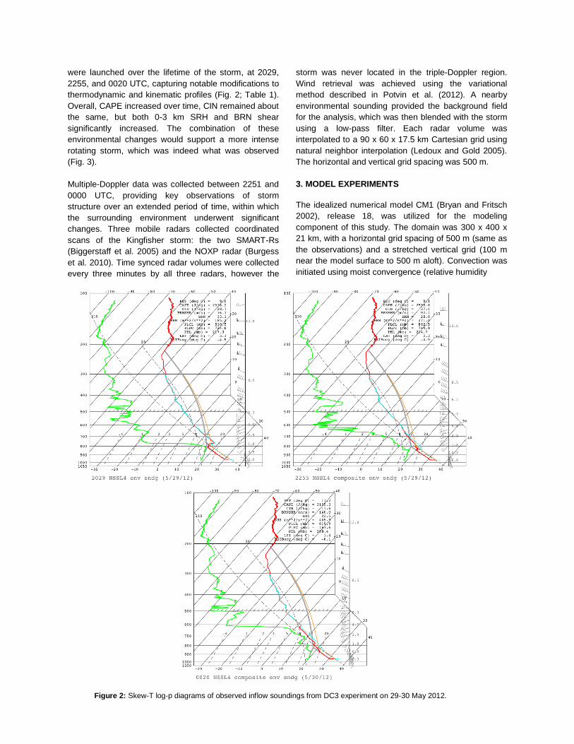
An overview of the simulation results in comparison to

the observations is shown in Fig. 3. It is evident in both

the control and BSS simulations that long-lived

supercells are produced, though their evolutions during

the observation period (2251 UTC corresponds to

approximately 3.5 hours into the simulations) are quite

different. Note that the observed supercell’s updraft

grew larger over time. In contrast, the control

simulation’s updraft grew smaller, and the size of the

storm overall also appears to shrink. The BSS supercell,

on the other hand, grows in size, as does its updraft.

Time-height plots of maximum vertical velocity and

maximum vertical vorticity further reveal differences in

the evolutions of the observed and simulated supercells.

Table 1: Evolution of select thermodynamic and kinematic

parameters associated with the soundings launched on 29-

30 May 2012; cf. Fig. 2.

Figure 3: Observed (top row) or simulated (middle and bottom rows) reflectivity (shaded). The 10 m/s vertical velocity contour at

5 km is indicated by the black line.

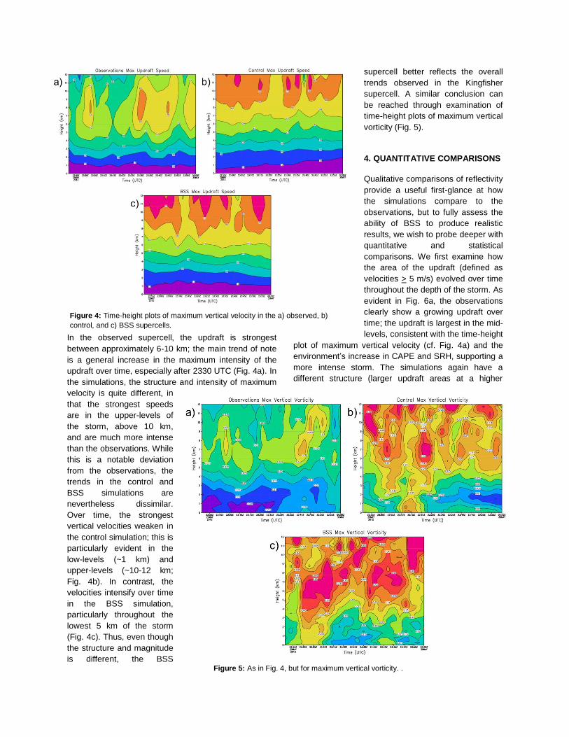
In the observed supercell, the updraft is strongest

between approximately 6-10 km; the main trend of note

is a general increase in the maximum intensity of the

updraft over time, especially after 2330 UTC (Fig. 4a). In

the simulations, the structure and intensity of maximum

velocity is quite different, in

that the strongest speeds

are in the upper-levels of

the storm, above 10 km,

and are much more intense

than the observations. While

this is a notable deviation

from the observations, the

trends in the control and

BSS simulations are

nevertheless dissimilar.

Over time, the strongest

vertical velocities weaken in

the control simulation; this is

particularly evident in the

low-levels (~1 km) and

upper-levels (~10-12 km;

Fig. 4b). In contrast, the

velocities intensify over time

in the BSS simulation,

particularly throughout the

lowest 5 km of the storm

(Fig. 4c). Thus, even though

the structure and magnitude

is different, the BSS

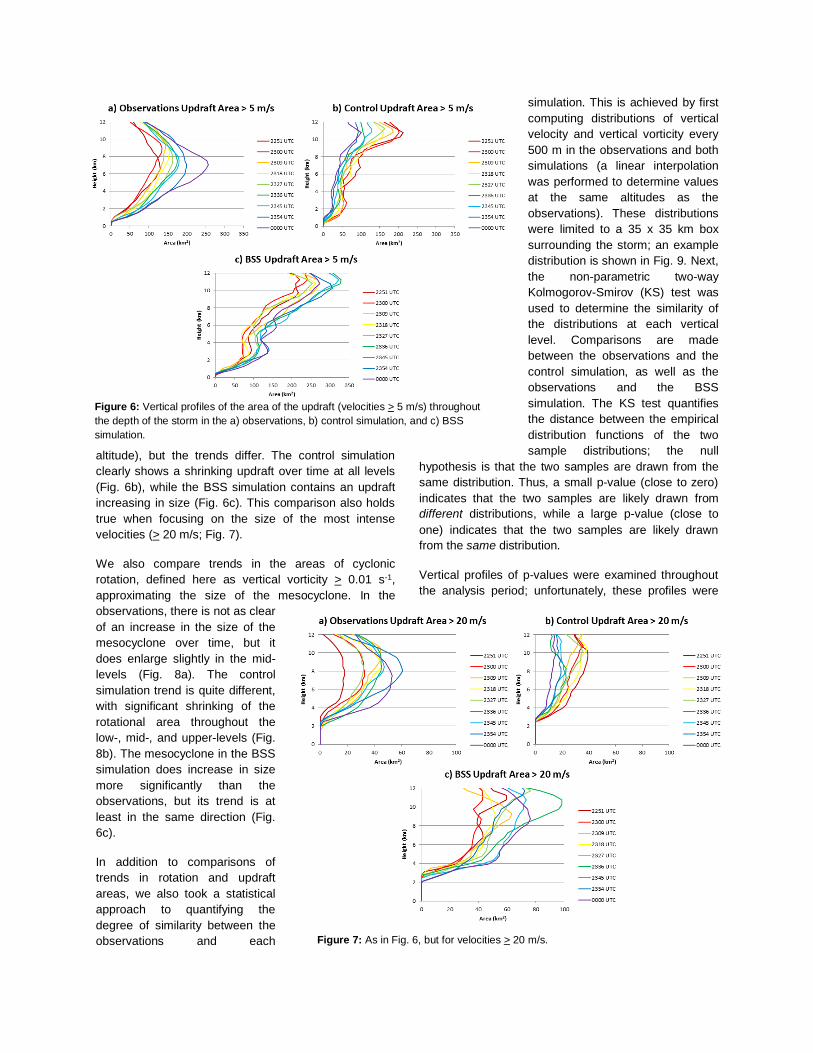
supercell better reflects the overall

trends observed in the Kingfisher

supercell. A similar conclusion can

be reached through examination of

time-height plots of maximum vertical

vorticity (Fig. 5).

4. QUANTITATIVE COMPARISONS

Qualitative comparisons of reflectivity

provide a useful first-glance at how

the simulations compare to the

observations, but to fully assess the

ability of BSS to produce realistic

results, we wish to probe deeper with

quantitative and statistical

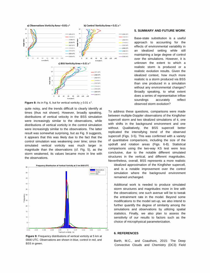
comparisons. We first examine how

the area of the updraft (defined as

velocities > 5 m/s) evolved over time

throughout the depth of the storm. As

evident in Fig. 6a, the observations

clearly show a growing updraft over

time; the updraft is largest in the mid-

levels, consistent with the time-height

plot of maximum vertical velocity (cf. Fig. 4a) and the

environment’s increase in CAPE and SRH, supporting a

more intense storm. The simulations again have a

different structure (larger updraft areas at a higher

Figure 4: Time-height plots of maximum vertical velocity in the a) observed, b)

control, and c) BSS supercells.

Figure 5: As in Fig. 4, but for maximum vertical vorticity. .

altitude), but the trends differ. The control simulation

clearly shows a shrinking updraft over time at all levels

(Fig. 6b), while the BSS simulation contains an updraft

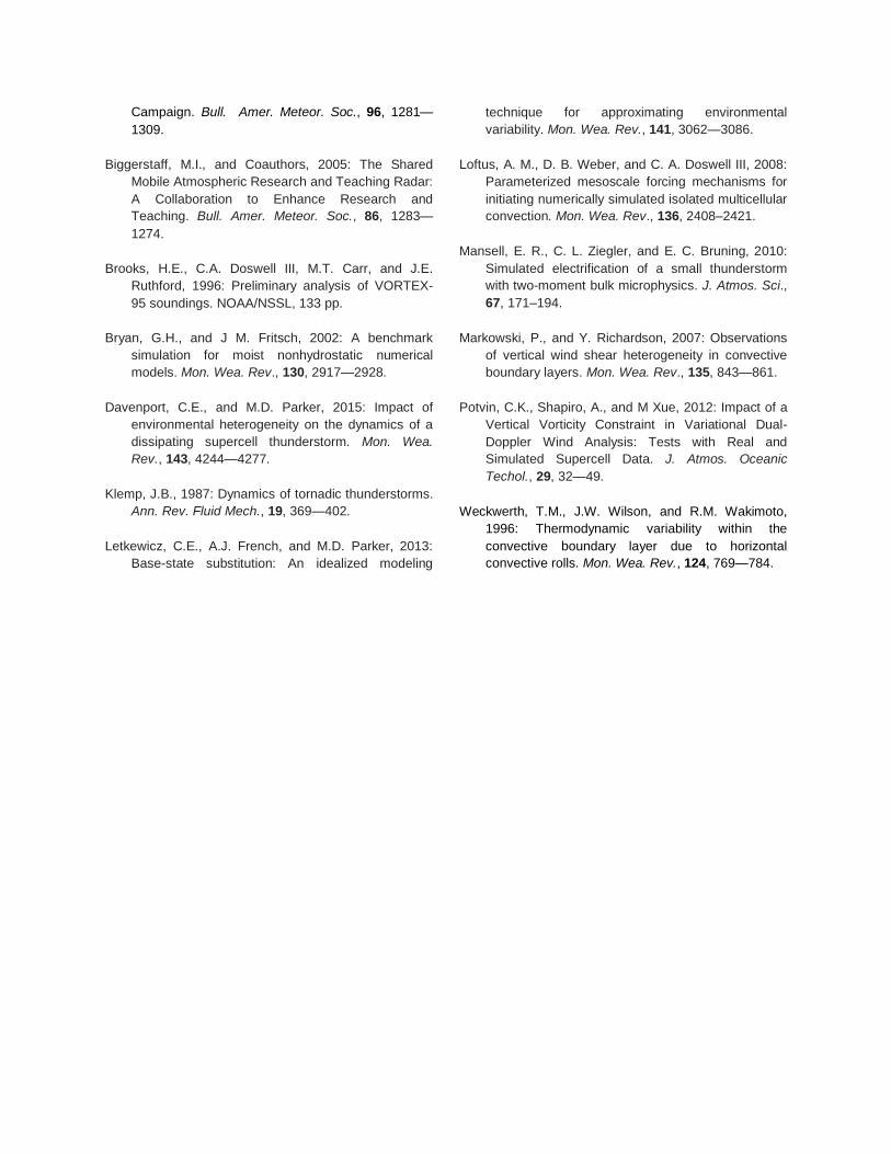
increasing in size (Fig. 6c). This comparison also holds

true when focusing on the size of the most intense

velocities (> 20 m/s; Fig. 7).

We also compare trends in the areas of cyclonic

rotation, defined here as vertical vorticity > 0.01 s-1,

approximating the size of the mesocyclone. In the

observations, there is not as clear

of an increase in the size of the

mesocyclone over time, but it

does enlarge slightly in the mid-

levels (Fig. 8a). The control

simulation trend is quite different,

with significant shrinking of the

rotational area throughout the

low-, mid-, and upper-levels (Fig.

8b). The mesocyclone in the BSS

simulation does increase in size

more significantly than the

observations, but its trend is at

least in the same direction (Fig.

6c).

In addition to comparisons of

trends in rotation and updraft

areas, we also took a statistical

approach to quantifying the

degree of similarity between the

observations and each

simulation. This is achieved by first

computing distributions of vertical

velocity and vertical vorticity every

500 m in the observations and both

simulations (a linear interpolation

was performed to determine values

at the same altitudes as the

observations). These distributions

were limited to a 35 x 35 km box

surrounding the storm; an example

distribution is shown in Fig. 9. Next,

the non-parametric two-way

Kolmogorov-Smirov (KS) test was

used to determine the similarity of

the distributions at each vertical

level. Comparisons are made

between the observations and the

control simulation, as well as the

observations and the BSS

simulation. The KS test quantifies

the distance between the empirical

distribution functions of the two

sample distributions; the null

hypothesis is that the two samples are drawn from the

same distribution. Thus, a small p-value (close to zero)

indicates that the two samples are likely drawn from

different distributions, while a large p-value (close to

one) indicates that the two samples are likely drawn

from the same distribution.

Vertical profiles of p-values were examined throughout

the analysis period; unfortunately, these profiles were

Figure 6: Vertical profiles of the area of the updraft (velocities > 5 m/s) throughout

the depth of the storm in the a) observations, b) control simulation, and c) BSS

simulation.

Figure 7: As in Fig. 6, but for velocities > 20 m/s.

quite noisy, and the trends difficult to clearly identify at

times (thus not shown). However, broadly speaking,

distributions of vertical velocity in the BSS simulation

were increasingly similar to the observations, while

distributions of vertical vorticity in the control simulation

were increasingly similar to the observations. The latter

result was somewhat surprising, but as Fig. 9 suggests,

it appears that this was likely due to the fact that the

control simulation was weakening over time; since the

simulated vertical vorticity was much larger in

magnitude than the observations (cf. Fig. 5), as the

storm weakened, its values became more in line with

the observations.

5. SUMMARY AND FUTURE WORK

Base-state substitution is a useful

approach to accounting for the

effects of environmental variability in

an idealized setting while still

maintaining a large degree of control

over the simulations. However, it is

unknown the extent to which a

realistic storm is produced or a

realistic evolution results. Given the

idealized context, how much more

realistic is a storm produced via BSS

than one produced in a simulation

without any environmental changes?

Broadly speaking, to what extent

does a series of representative inflow

soundings accurately reflect

observed storm evolution?

To address these questions, comparisons were made

between multiple-Doppler observations of the Kingfisher

supercell storm and two idealized simulations of it, one

with shifts in the background environment and one

without. Qualitatively, the BSS supercell better

replicated the intensifying trend of the observed

supercell (Figs. 3-5). This was confirmed with a variety

of quantitative comparisons, including the size of the

updraft and rotation areas (Figs. 6-8). Statistical

comparisons using the two-way KS test were less

conclusive, due to the notable different simulated

structures in the vertical, and different magnitudes.

Nevertheless, overall, BSS represents a more realistic

idealized approximation of the Kingfisher supercell,

and is a notable improvement over the control

simulation where the background environment

remained unchanged.

Additional work is needed to produce simulated

storm structures and magnitudes more in line with

the observations; one such avenue will be to tweak

the entrainment rate in the model. Beyond some

modifications to the model set-up, we also intend to

further quantify the degree of similarity among the

simulations and observations by utilizing spatial

statistics. Finally, we also plan to assess the

sensitivity of our results to factors such as the

choice of microphysical parameterization.

6. REFERENCES

Barth, M.C., and Coauthors, 2015: The Deep

Convective Clouds and Chemistry (DC3) Field

Figure 8: As in Fig. 6, but for vertical vorticity > 0.01 s-1.

Figure 9: Frequency distributions of vertical vorticity at 5 km at

0000 UTC. Observations are shown in blue, control in red, and

BSS in green.

Campaign. Bull. Amer. Meteor. Soc., 96, 1281—

1309.

Biggerstaff, M.I., and Coauthors, 2005: The Shared

Mobile Atmospheric Research and Teaching Radar:

A Collaboration to Enhance Research and

Teaching. Bull. Amer. Meteor. Soc., 86, 1283—

1274.

Brooks, H.E., C.A. Doswell III, M.T. Carr, and J.E.

Ruthford, 1996: Preliminary analysis of VORTEX-

95 soundings. NOAA/NSSL, 133 pp.

Bryan, G.H., and J M. Fritsch, 2002: A benchmark

simulation for moist nonhydrostatic numerical

models. Mon. Wea. Rev., 130, 2917—2928.

Davenport, C.E., and M.D. Parker, 2015: Impact of

environmental heterogeneity on the dynamics of a

dissipating supercell thunderstorm. Mon. Wea.

Rev., 143, 4244—4277.

Klemp, J.B., 1987: Dynamics of tornadic thunderstorms.

Ann. Rev. Fluid Mech., 19, 369—402.

Letkewicz, C.E., A.J. French, and M.D. Parker, 2013:

Base-state substitution: An idealized modeling

technique for approximating environmental

variability. Mon. Wea. Rev., 141, 3062—3086.

Loftus, A. M., D. B. Weber, and C. A. Doswell III, 2008:

Parameterized mesoscale forcing mechanisms for

initiating numerically simulated isolated multicellular

convection. Mon. Wea. Rev., 136, 2408–2421.

Mansell, E. R., C. L. Ziegler, and E. C. Bruning, 2010:

Simulated electrification of a small thunderstorm

with two-moment bulk microphysics. J. Atmos. Sci.,

67, 171–194.

Markowski, P., and Y. Richardson, 2007: Observations

of vertical wind shear heterogeneity in convective

boundary layers. Mon. Wea. Rev., 135, 843—861.

Potvin, C.K., Shapiro, A., and M Xue, 2012: Impact of a

Vertical Vorticity Constraint in Variational Dual-

Doppler Wind Analysis: Tests with Real and

Simulated Supercell Data. J. Atmos. Oceanic

Techol., 29, 32—49.

Weckwerth, T.M., J.W. Wilson, and R.M. Wakimoto,

1996: Thermodynamic variability within the

convective boundary layer due to horizontal

convective rolls. Mon. Wea. Rev., 124, 769—784.