Embed Size (px)
Citation preview
04/19/23http://
numericalmethods.eng.usf.edu 1
Nonlinear Regression
Chemical Engineering Majors
Authors: Autar Kaw, Luke Snyder
http://numericalmethods.eng.usf.eduTransforming Numerical Methods Education for STEM
Undergraduates
Nonlinear Regression
http://numericalmethods.eng.usf.edu
Nonlinear Regression
)( bxaey
)( baxy
xb
axy
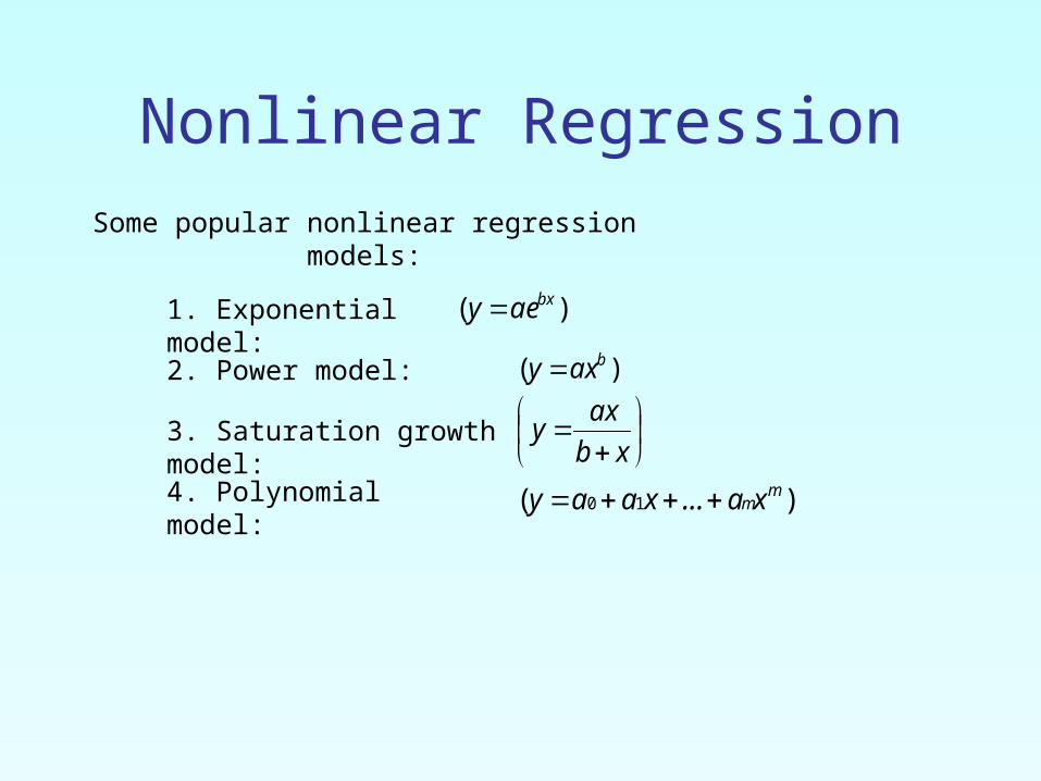
Some popular nonlinear regression models:
1. Exponential model:2. Power model:
3. Saturation growth model:4. Polynomial model: )( 10
mmxa...xaay
Nonlinear Regression
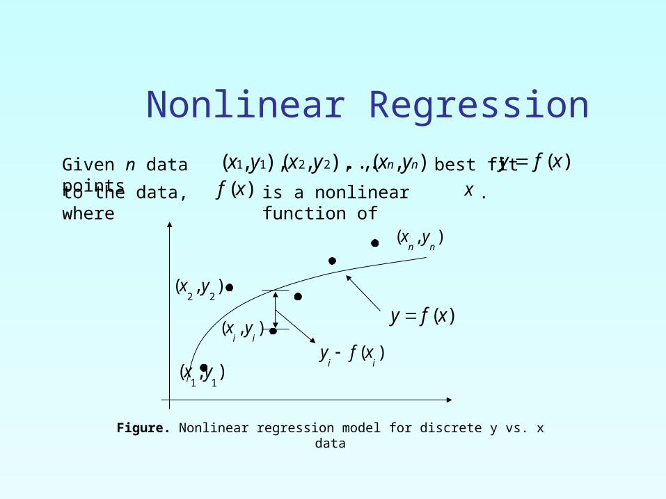
Given n data points
),( , ... ),,(),,( 2211 nn yxyx yx best fit )(xfy
to the data, where
)(xf is a nonlinear function of
x .
Figure. Nonlinear regression model for discrete y vs. x data
)(xfy
),(nn
yx
),(11
yx
),(22
yx
),(ii
yx
)(ii
xfy
RegressionExponential Model
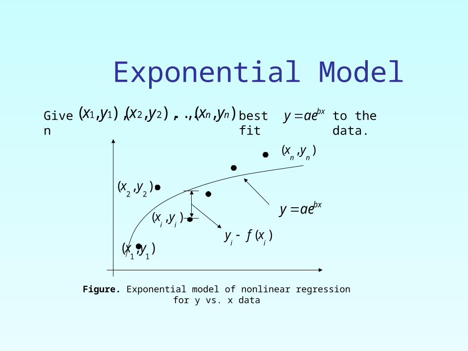
Exponential Model),( , ... ),,(),,( 2211 nn yxyx yxGive
nbest fit
bxaey to the data.
Figure. Exponential model of nonlinear regression for y vs. x data
bxaey
),(nn
yx
),(11
yx
),(22
yx
),(ii
yx
)(ii
xfy
Finding constants of Exponential Model
n
i
bx
ir iaeyS
1
2
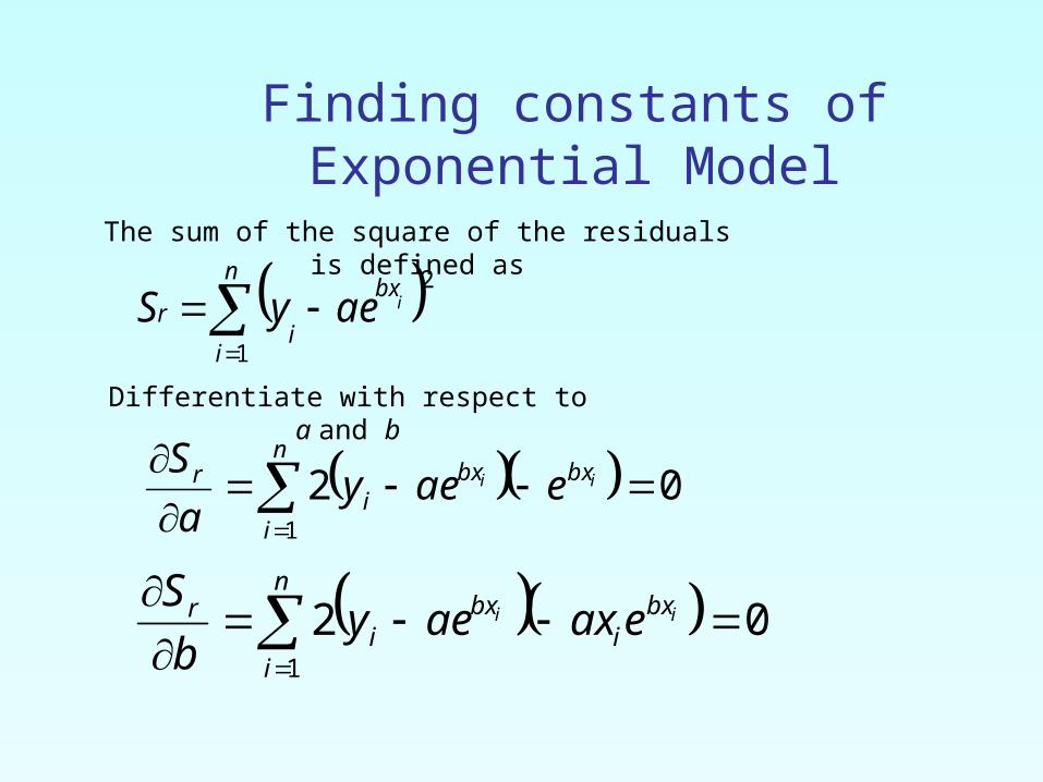
The sum of the square of the residuals is defined as
Differentiate with respect to a and b
021
ii bxn
i
bxi
r eaeya
S
021
ii bxi
n
i
bxi
r eaxaeyb
S
Finding constants of Exponential Model
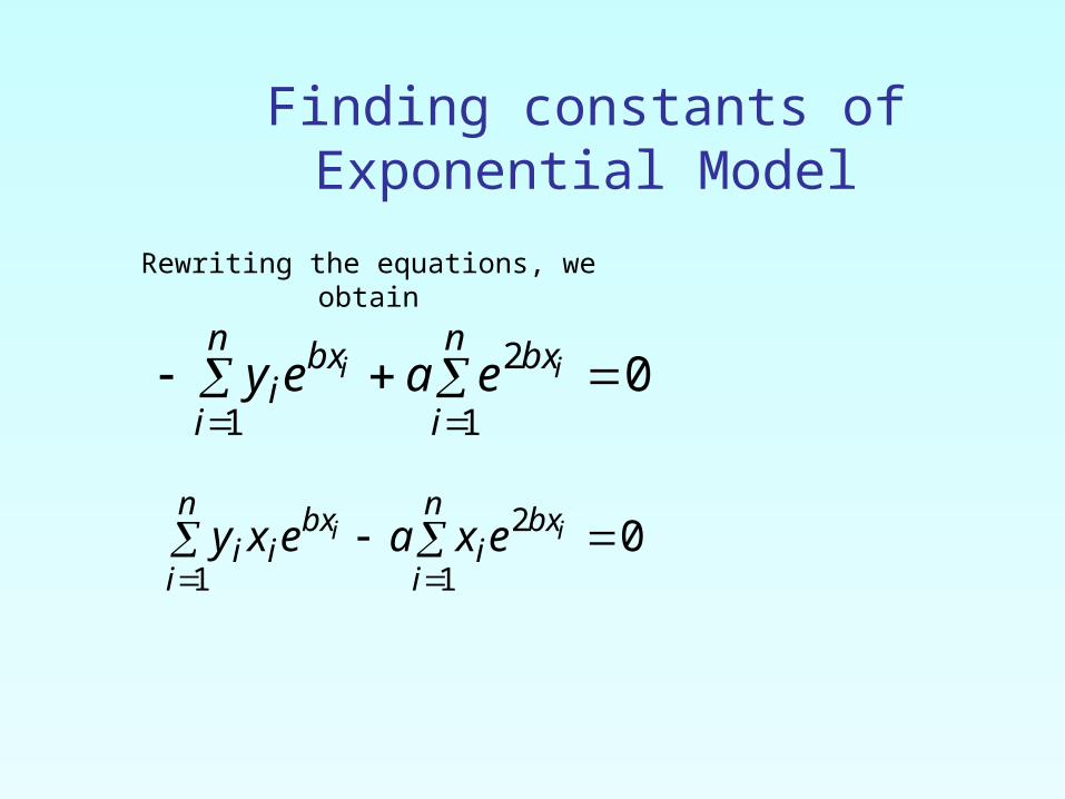
Rewriting the equations, we obtain
01
2
1
n
i
bxn
i
bxi
ii eaey
01
2
1
n
i
bxi
n
i
bxii
ii exaexy
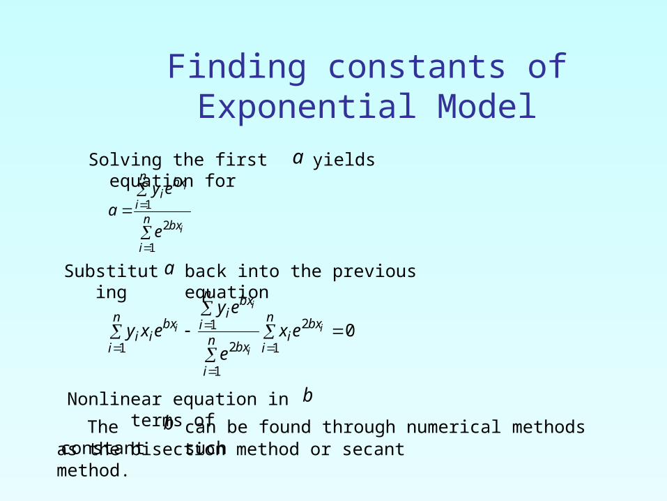
Finding constants of Exponential Model
Substituting
a back into the previous equation
01
2
1
2
1
1
n
i
bxin
i
bx
bxn
ii
bxi
n
ii
i
i
i
i exe
eyexy
The constant
b can be found through numerical methods suchas the bisection method or secant method.
Nonlinear equation in terms of
b
n
i
bx
n
i
bxi
i
i
e
eya
1
2
1
Solving the first equation for
a yields
Example 1-Exponential Model
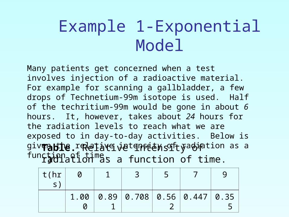
t(hrs) 0 1 3 5 7 9
1.000 0.891 0.708 0.562 0.447 0.355
Many patients get concerned when a test involves injection of a radioactive material. For example for scanning a gallbladder, a few drops of Technetium-99m isotope is used. Half of the techritium-99m would be gone in about 6 hours. It, however, takes about 24 hours for the radiation levels to reach what we are exposed to in day-to-day activities. Below is given the relative intensity of radiation as a function of time.
Table. Relative intensity of radiation as a function of time.
Example 1-Exponential Model cont.
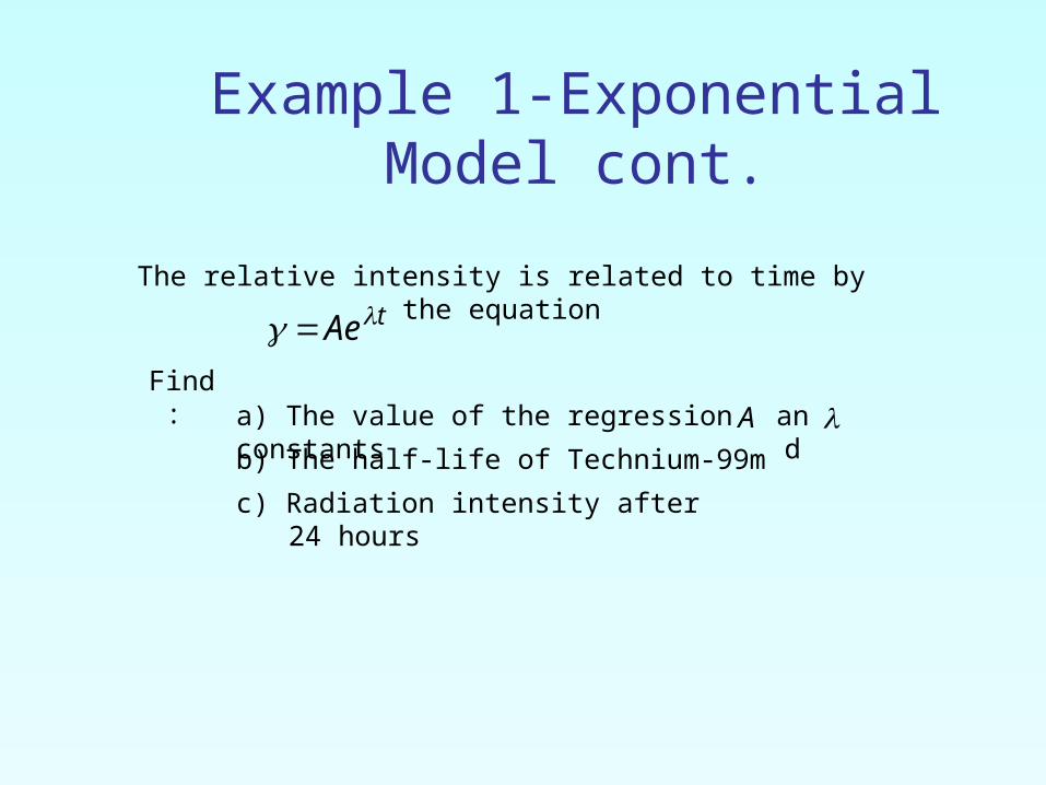
Find: a) The value of the regression
constants A an
db) The half-life of Technium-99m
c) Radiation intensity after 24 hours
The relative intensity is related to time by the equationtAe
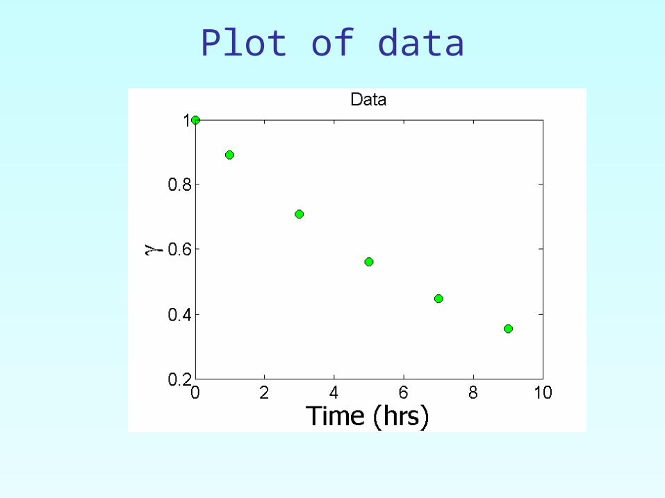
Plot of data
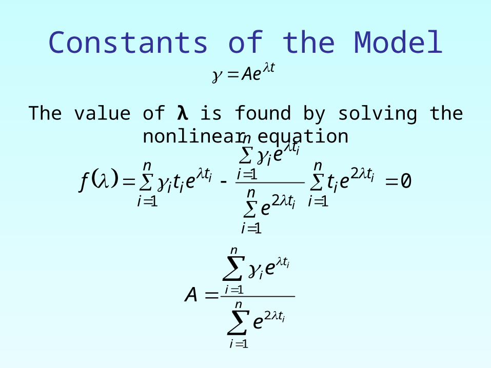
Constants of the Model
The value of λ is found by solving the nonlinear equation
01
2
1
2
1
1
n
i
tin
i
t
n
i
ti
ti
n
ii
i
i
i
i ete
eetf
n
i
t
n
i
ti
i
i
e
eA
1
2
1
tAe
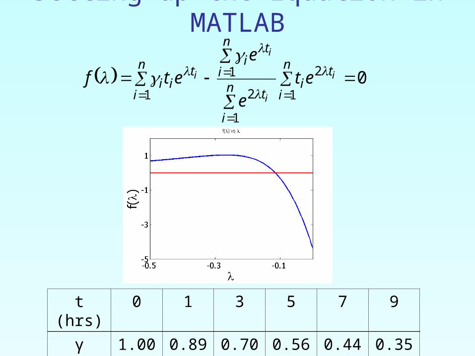
Setting up the Equation in MATLAB
01
2
1
2
1
1
n
i
tin
i
t
n
i
ti
ti
n
ii
i
i
i
i ete
eetf
t (hrs) 0 1 3 5 7 9
γ 1.000
0.891
0.708
0.562
0.447
0.355
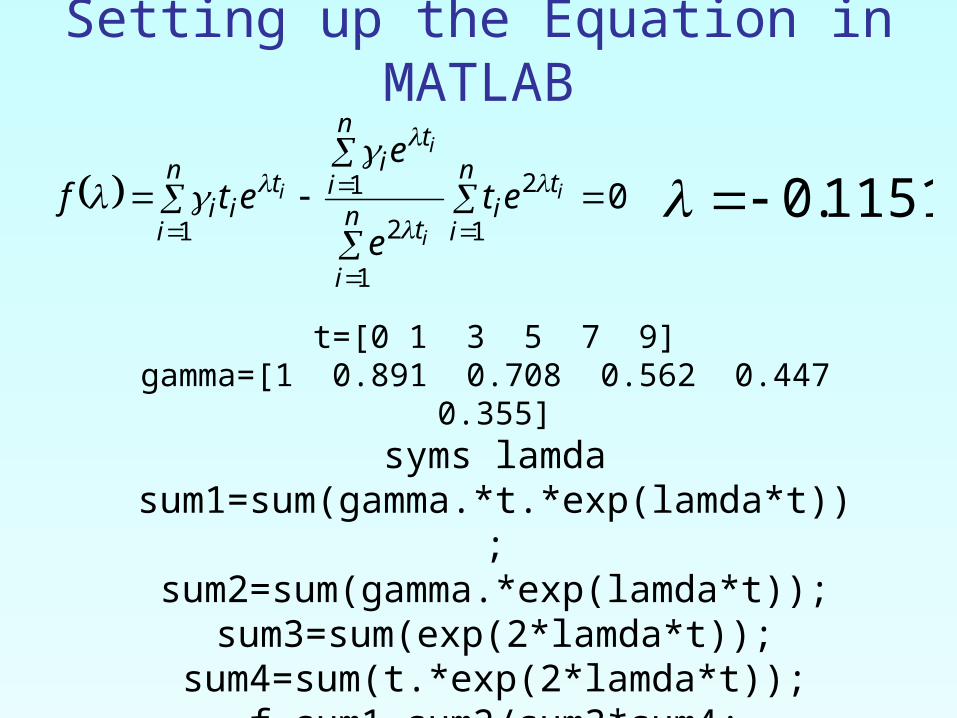
Setting up the Equation in MATLAB
01
2
1
2
1
1
n
i
tin
i
t
n
i
ti
ti
n
ii
i
i
i
i ete
eetf
t=[0 1 3 5 7 9]gamma=[1 0.891 0.708 0.562 0.447
0.355]syms lamda
sum1=sum(gamma.*t.*exp(lamda*t));
sum2=sum(gamma.*exp(lamda*t));sum3=sum(exp(2*lamda*t));
sum4=sum(t.*exp(2*lamda*t));f=sum1-sum2/sum3*sum4;
1151.0
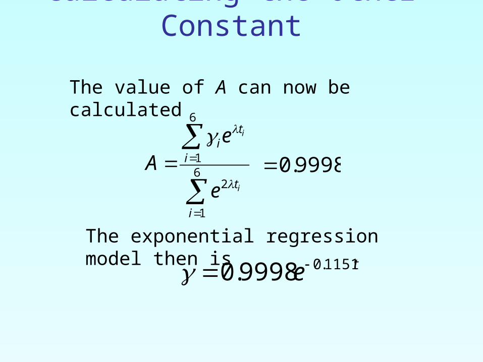
Calculating the Other Constant
The value of A can now be calculated
6
1
2
6
1
i
t
i
ti
i
i
e
eA
9998.0
The exponential regression model then is te 1151.0 9998.0
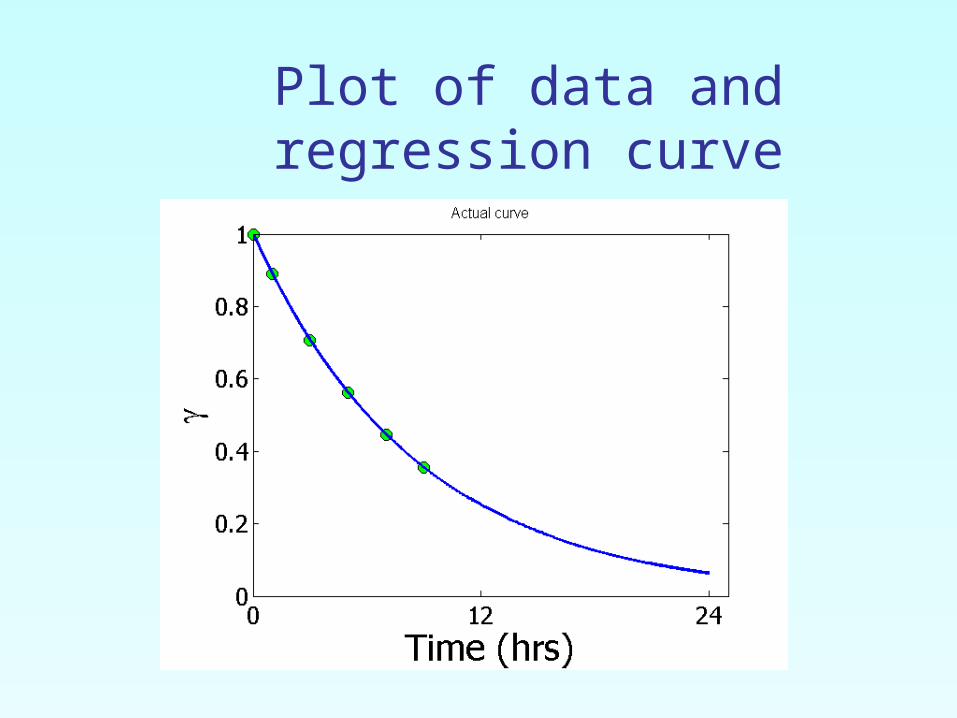
Plot of data and regression curve
te 1151.0 9998.0
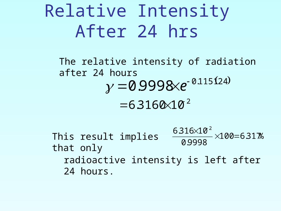
Relative Intensity After 24 hrs
The relative intensity of radiation after 24 hours
241151.09998.0 e2103160.6
This result implies that only
%317.61009998.0
10316.6 2
radioactive intensity is left after 24 hours.
Homework1. What is the half-life of
technetium 99m isotope?
2. Compare the constants of this regression model with the one where the data is transformed.
3. Write a program in the language of your choice to find the constants of the model.
THE END
http://numericalmethods.eng.usf.edu
Polynomial Model
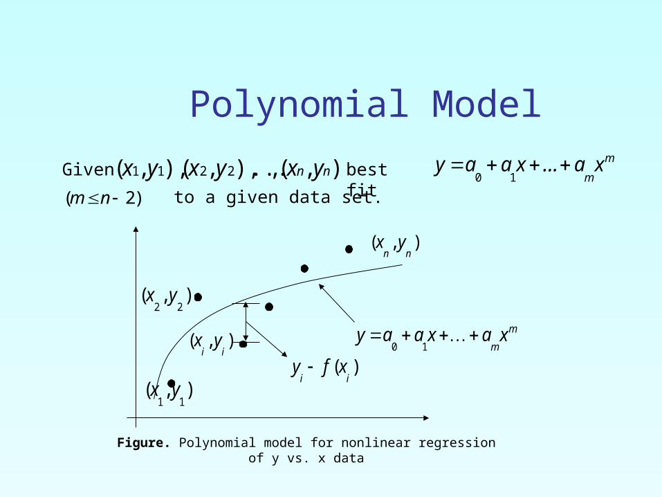
),( , ... ),,(),,( 2211 nn yxyx yxGiven best fit
m
mxa...xaay
10
)2( nm to a given data set.
Figure. Polynomial model for nonlinear regression of y vs. x data
m
mxaxaay
10
),(nn
yx
),(11
yx
),(22
yx
),(ii
yx
)(ii
xfy
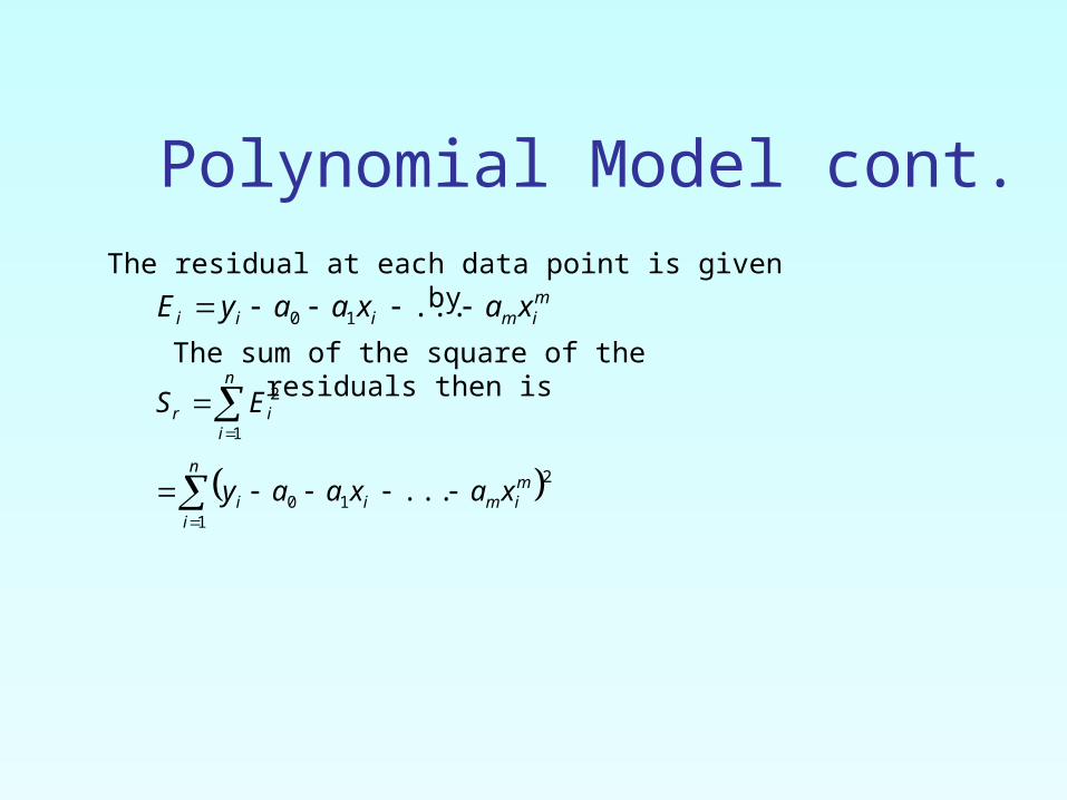
Polynomial Model cont.The residual at each data point is given by
mimiii xaxaayE ...10
The sum of the square of the residuals then is
n
i
mimii
n
iir
xaxaay
ES
1
2
10
1
2
...
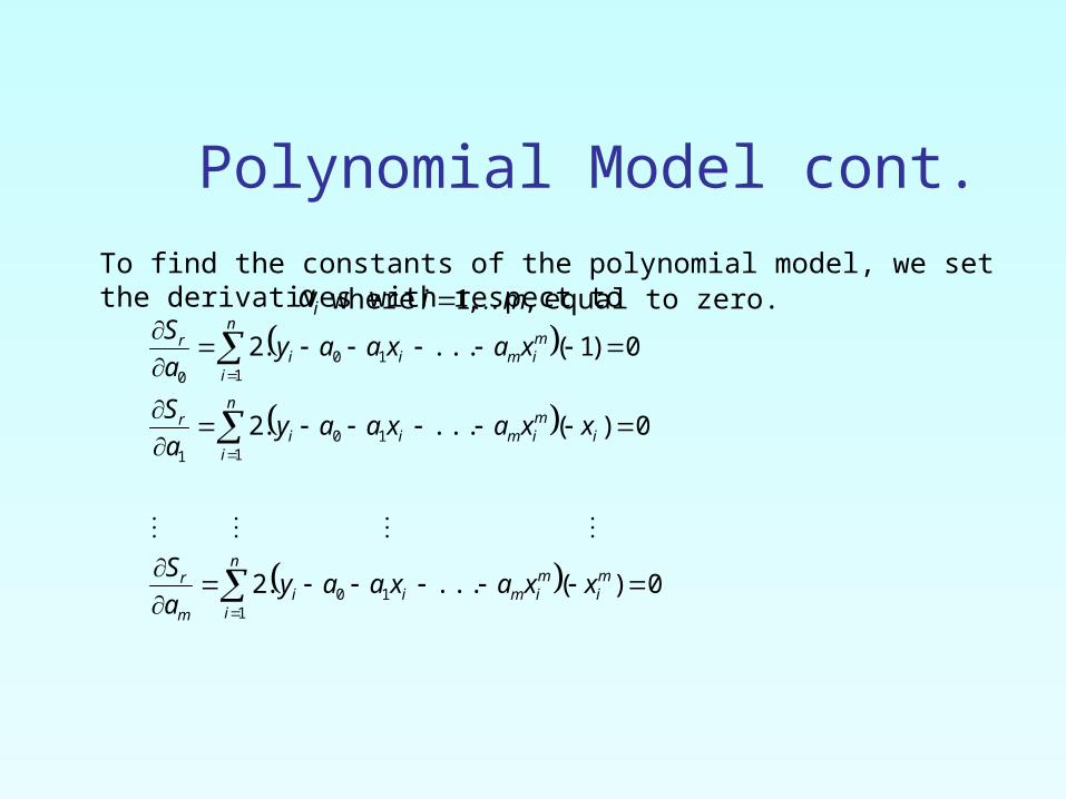
Polynomial Model cont.To find the constants of the polynomial model, we set the derivatives with respect to ia wher
e
0)(....2
0)(....2
0)1(....2
110
110
1
110
0
mi
n
i
mimii
m
r
i
n
i
mimii
r
n
i
mimii
r
xxaxaaya
S
xxaxaaya
S
xaxaaya
S
,,1 mi equal to zero.
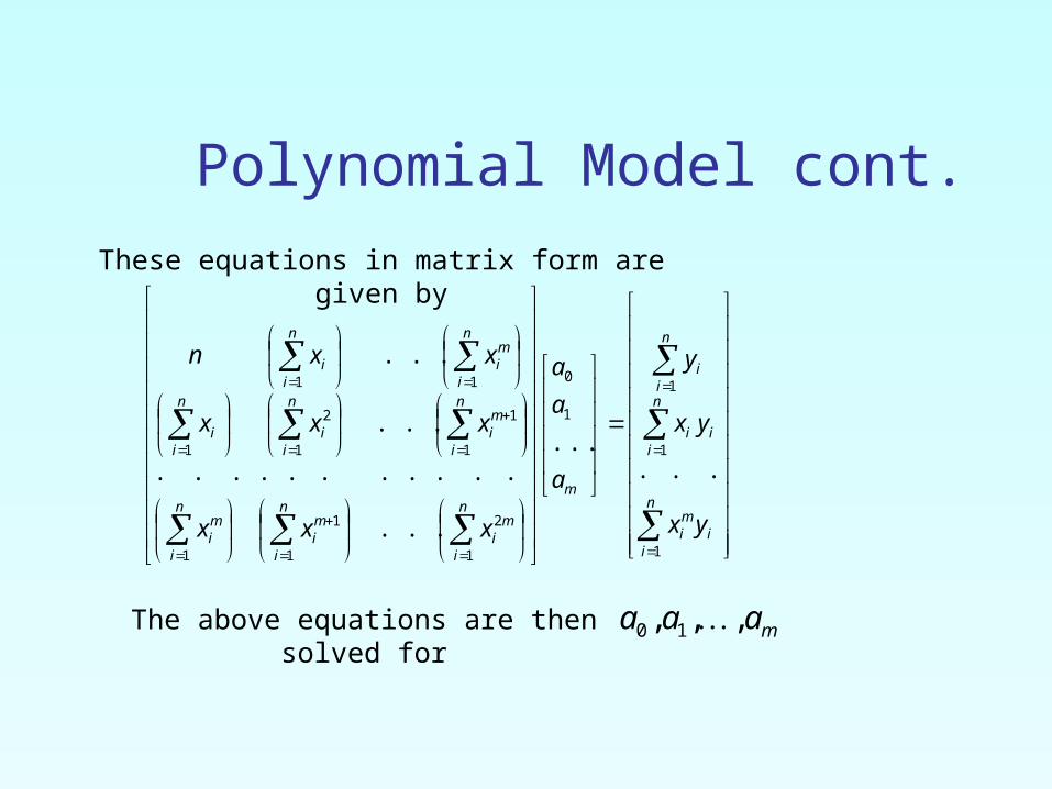
Polynomial Model cont.These equations in matrix form are
given by
n
ii
mi
n
iii
n
ii
mn
i
mi
n
i
mi
n
i
mi
n
i
mi
n
ii
n
ii
n
i
mi
n
ii
yx
yx
y
a
a
a
xxx
xxx
xxn
1
1
1
1
0
1
2
1
1
1
1
1
1
2
1
11
......
...
...........
...
...
The above equations are then solved for
maaa ,,, 10
http://numericalmethods.eng.usf.edu 25
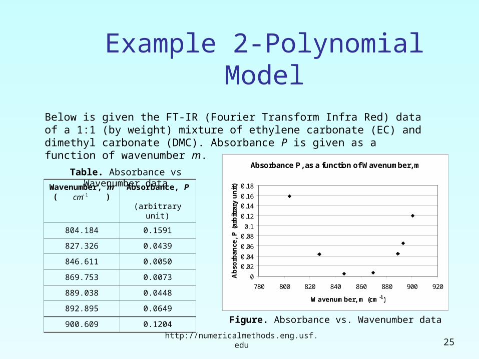
Example 2-Polynomial ModelBelow is given the FT-IR (Fourier Transform Infra Red) data of a 1:1 (by weight) mixture of ethylene carbonate (EC) and dimethyl carbonate (DMC). Absorbance P is given as a function of wavenumber m.
Wavenumber, m( )
Absorbance, P (arbitrary unit)
804.184 0.1591
827.326 0.0439
846.611 0.0050
869.753 0.0073
889.038 0.0448
892.895 0.0649
900.609 0.1204
Absorbance P, as a function of Wavenumber, m
0
0.02
0.04
0.06
0.08
0.1
0.12
0.14
0.16
0.18
780 800 820 840 860 880 900 920
Wavenumber, m (cm-1)
Ab
sorb
ance
, P
(ar
bit
rary
un
it)
Table. Absorbance vs Wavenumber data
Figure. Absorbance vs. Wavenumber data
1cm
http://numericalmethods.eng.usf.edu 26
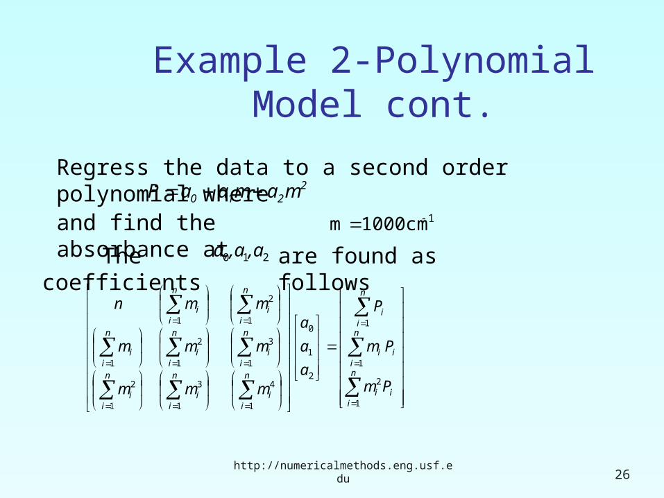
Example 2-Polynomial Model cont.
Regress the data to a second order polynomial where 2
210 mamaaP
and find the absorbance at
11000cmm
The coefficients 210 ,a,aa are found as follows
n
iii
n
iii
n
ii
n
ii
n
ii
n
ii
n
ii
n
ii
n
ii
n
ii
n
ii
Pm
Pm
P
a
a
a
mmm
mmm
mmn
1
2
1
1
2
1
0
1
4
1
3
1
2
1
3
1
2
1
1
2
1
http://numericalmethods.eng.usf.edu 27
Example 2-Polynomial Model cont.
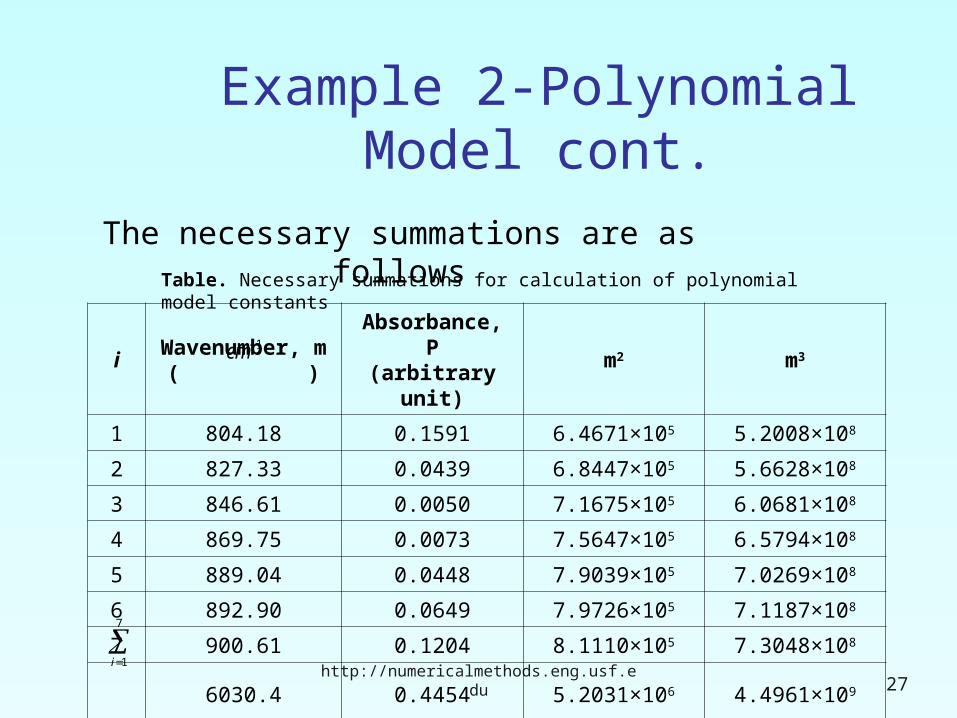
The necessary summations are as follows
iWavenumber, m
( )Absorbance, P(arbitrary unit)
m2 m3
1 804.18 0.1591 6.4671×10⁵ 5.2008×10⁸
2 827.33 0.0439 6.8447×10⁵ 5.6628×10⁸
3 846.61 0.0050 7.1675×10⁵ 6.0681×10⁸
4 869.75 0.0073 7.5647×10⁵ 6.5794×10⁸
5 889.04 0.0448 7.9039×10⁵ 7.0269×10⁸
6 892.90 0.0649 7.9726×10⁵ 7.1187×10⁸
7 900.61 0.1204 8.1110×10⁵ 7.3048×10⁸
6030.4 0.4454 5.2031×10⁶ 4.4961×10⁹
Table. Necessary summations for calculation of polynomial model constants
1cm
7
1i
http://numericalmethods.eng.usf.edu 28
Example 2-Polynomial Model cont.
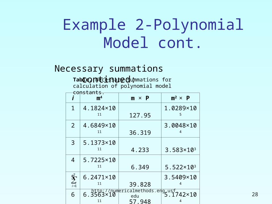
Necessary summations continued:
i m4 m × P m2 × P
1 4.1824×10¹¹ 127.95 1.0289×10⁵
2 4.6849×10¹¹ 36.319 3.0048×10⁴
3 5.1373×10¹¹ 4.233 3.583×10³
4 5.7225×10¹¹ 6.349 5.522×10³
5 6.2471×10¹¹ 39.828 3.5409×10⁴
6 6.3563×10¹¹ 57.948 5.1742×10⁴
7 6.5787×10¹¹ 108.43 9.7655×10⁴
3.8909×10¹² 381.06 3.2685×10⁵
Table. Necessary summations for calculation of polynomial model constants.
7
1i
http://numericalmethods.eng.usf.edu 29
Example 2-Polynomial Model cont.
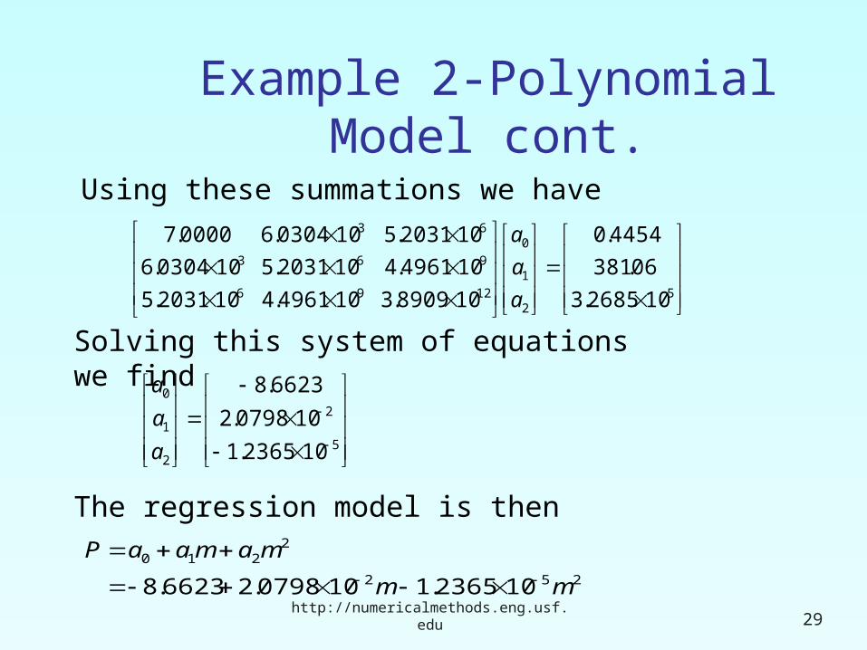
Using these summations we have
52
1
0
1296
963
63
102685.3
06.381
4454.0
108909.3104961.4102031.5
104961.4102031.5100304.6
102031.5100304.60000.7
a
a
a
Solving this system of equations we find
5
2
2
1
0
102365.1
100798.2
6623.8
a
a
a
The regression model is then
252
2210
102365.1100798.26623.8 mm
mamaaP
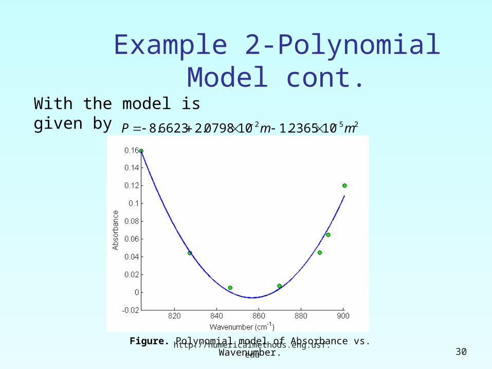
252 102365.1100798.26623.8 mmP
http://numericalmethods.eng.usf.edu 30
Example 2-Polynomial Model cont.
With the model is given by
Figure. Polynomial model of Absorbance vs. Wavenumber.
http://numericalmethods.eng.usf.edu 31
Example 2-Polynomial Model cont.
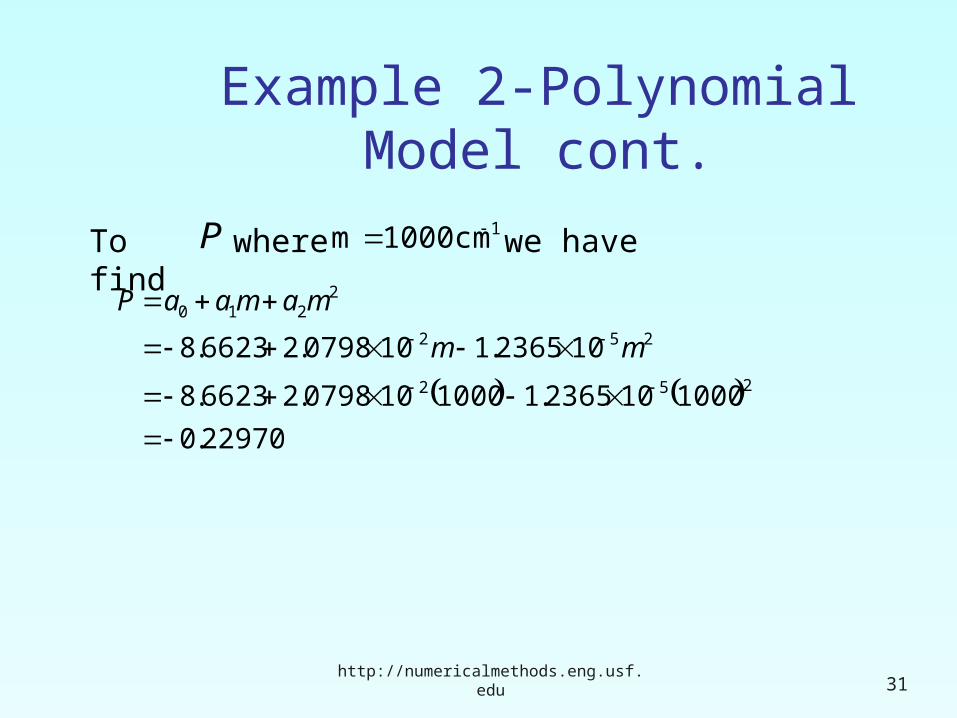
To find P where 11000cmm we have
22970.0
1000102365.11000100798.26623.8
102365.1100798.26623.8252
252
2210
mm
mamaaP
yz ln
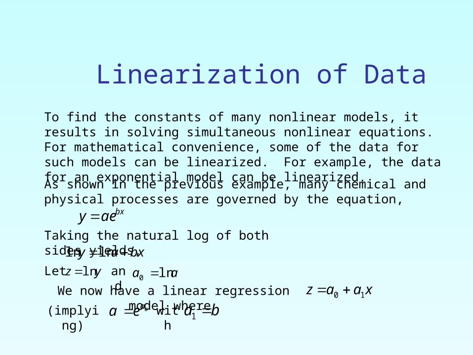
Linearization of DataTo find the constants of many nonlinear models, it results in solving simultaneous nonlinear equations. For mathematical convenience, some of the data for such models can be linearized. For example, the data for an exponential model can be linearized.As shown in the previous example, many chemical and physical processes are governed by the equation,
bxaey Taking the natural log of both sides yields, bxay lnln
Let and
aa ln0
(implying)
oaea with
ba 1
We now have a linear regression model where
xaaz 10
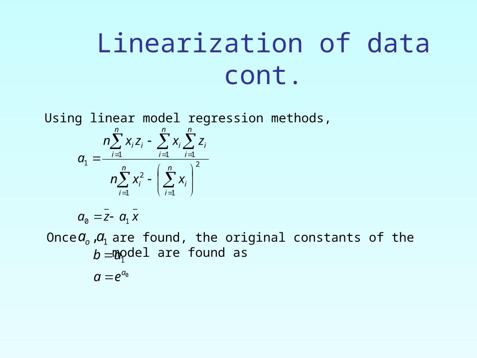
Linearization of data cont.Using linear model regression methods,
_
1
_
0
1
2
1
2
11 11
xaza
xxn
zxzxna
n
i
n
iii
n
ii
n
i
n
iiii
Once 1,aao are found, the original constants of the model are found as
0
1
aea
ab
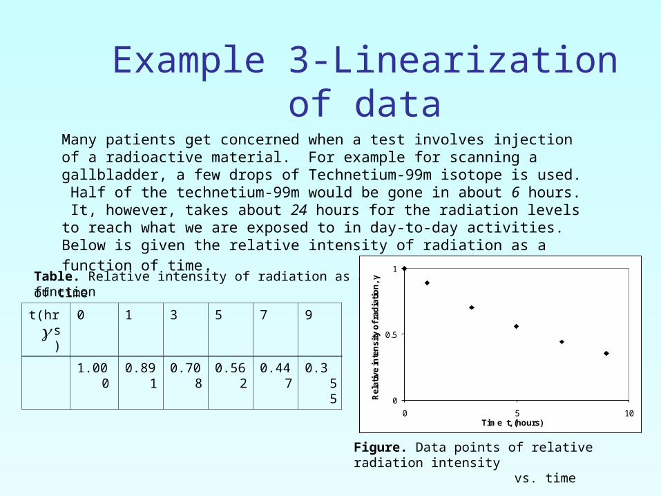
Example 3-Linearization of data
t(hrs) 0 1 3 5 7 9
1.000 0.891 0.708 0.562 0.447 0.355
Many patients get concerned when a test involves injection of a radioactive material. For example for scanning a gallbladder, a few drops of Technetium-99m isotope is used. Half of the technetium-99m would be gone in about 6 hours. It, however, takes about 24 hours for the radiation levels to reach what we are exposed to in day-to-day activities. Below is given the relative intensity of radiation as a function of time.
Table. Relative intensity of radiation as a function
of time
0
0.5
1
0 5 10
Rel
ativ
e in
ten
sity
of r
adia
tio
n, γ
Time t, (hours)
Figure. Data points of relative radiation intensity
vs. time
Example 3-Linearization of data cont.
Find: a) The value of the regression
constants A an
db) The half-life of Technium-99m
c) Radiation intensity after 24 hours
The relative intensity is related to time by the equation tAe
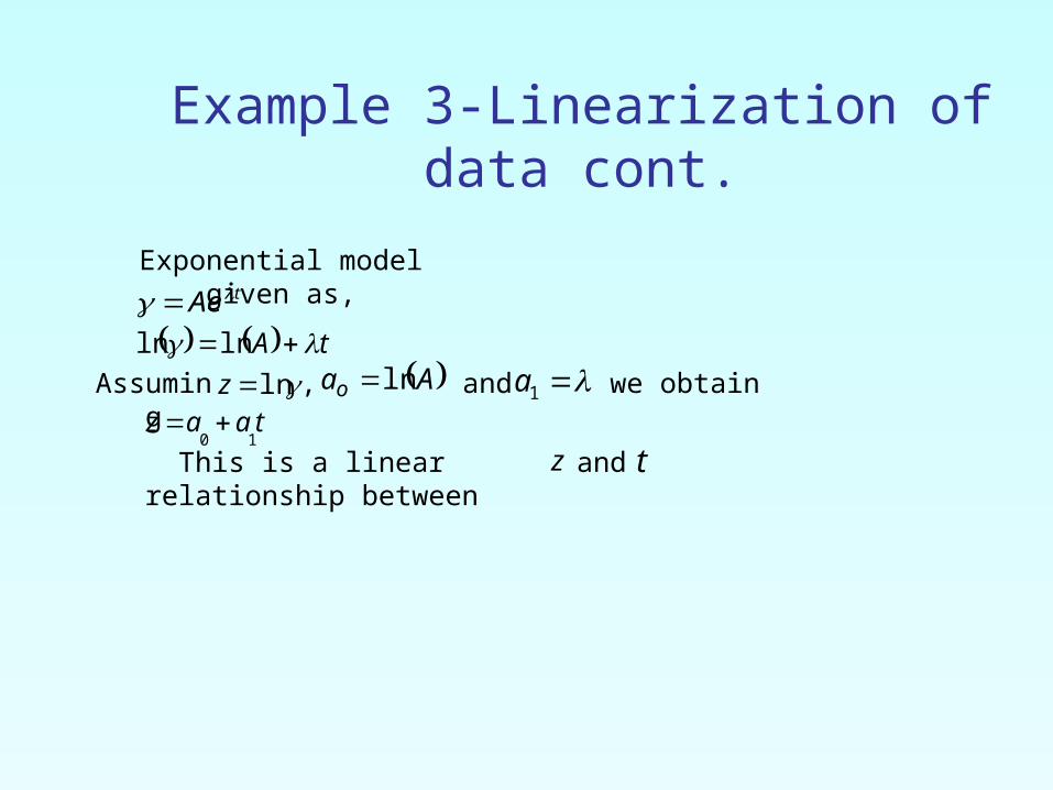
Example 3-Linearization of data cont.
tAe Exponential model given
as,
tA lnln
Assuming
lnz , Aao ln and 1a we obtaintaaz
10
This is a linear relationship between
z and t
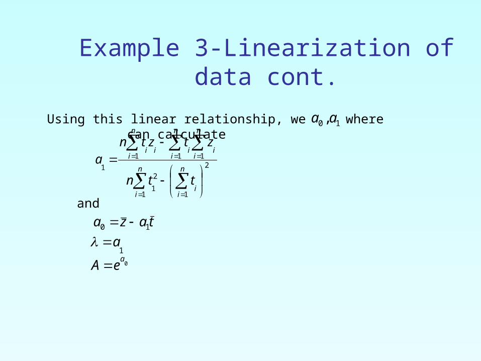
Example 3-Linearization of data cont.
Using this linear relationship, we can calculate
10 , aa
n
i
n
ii
n
ii
n
i
n
iiii
ttn
ztztna
1
2
1
2
1
11 1
1
and
taza 10
where
1a
0a
eA
Example 3-Linearization of Data cont.
123456
013579
10.8910.7080.5620.4470.355
0.00000−0.11541−0.34531−0.57625−0.80520−1.0356
0.0000−0.11541−1.0359−2.8813−5.6364−9.3207
0.00001.00009.000025.00049.00081.000
25.000 −2.8778 −18.990 165.00
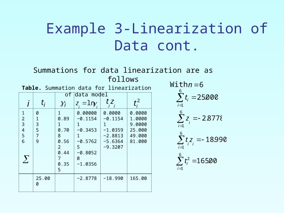
Summations for data linearization are as follows
Table. Summation data for linearization of data model
i it iii
z ln iizt 2
it
With 6n
000.256
1
i
it
6
1
8778.2i
iz
6
1
990.18i
iizt
00.1656
1
2 i
it
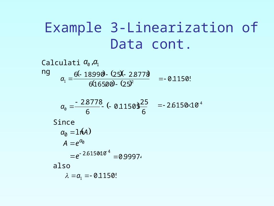
Example 3-Linearization of Data cont.
Calculating 10 ,aa
21
2500.1656
8778.225990.186
a 11505.0
6
2511505.0
6
8778.20
a
4106150.2
Since Aa ln0 0aeA
4106150.2 e 99974.0
11505.01 aalso
Example 3-Linearization of Data cont.
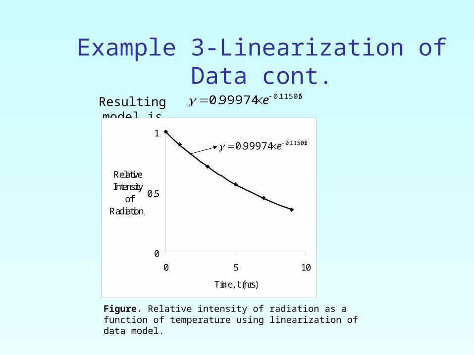
Resulting model is
te 11505.099974.0
0
0.5
1
0 5 10
Time, t (hrs)
Relative Intensity
of Radiation,
te 11505.099974.0
Figure. Relative intensity of radiation as a function of temperature using linearization of data model.
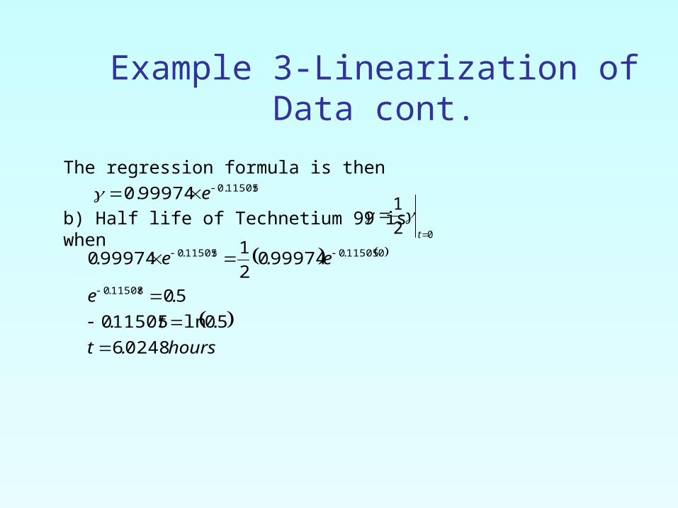
Example 3-Linearization of Data cont.
The regression formula is thente 11505.099974.0
b) Half life of Technetium 99 is when02
1
t
hours.t
.t.
.e
e.e.
t.
.t.
02486
50ln115050
50
9997402
1999740
115080
0115050115050
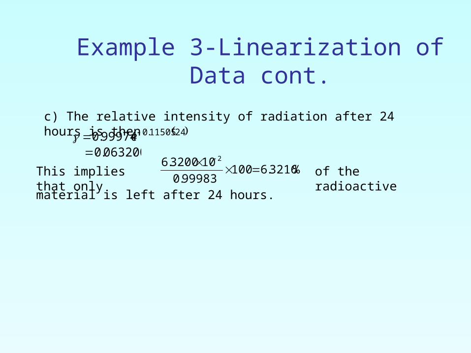
Example 3-Linearization of Data cont.
c) The relative intensity of radiation after 24 hours is then 2411505.099974.0 e
063200.0This implies that only
%3216.610099983.0
103200.6 2
of the radioactive
material is left after 24 hours.
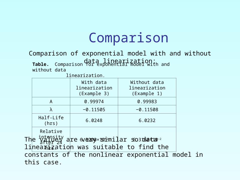
Comparison Comparison of exponential model with and without data
linearization:
With data linearization(Example 3)
Without data linearization(Example 1)
A 0.99974 0.99983
λ −0.11505 −0.11508
Half-Life (hrs) 6.0248 6.0232
Relative intensity after 24 hrs.
6.3200×10⁻² 6.3160×10⁻²
Table. Comparison for exponential model with and without data linearization.
The values are very similar so data linearization was suitable to find the constants of the nonlinear exponential model in this case.

Additional ResourcesFor all resources on this topic such as digital audiovisual lectures, primers, textbook chapters, multiple-choice tests, worksheets in MATLAB, MATHEMATICA, MathCad and MAPLE, blogs, related physical problems, please visit
http://numericalmethods.eng.usf.edu/topics/nonlinear_regression.html