Embed Size (px)
Citation preview

RANSAC16-385 Computer Vision (Kris Kitani)
Carnegie Mellon University

Up to now, we’ve assumed correct correspondences

What if there are mismatches?
outlier
How would you find just the inliers?

RANSAC RANdom SAmple Consensus
[Fischler & Bolles in ’81]

Algorithm:1. Sample (randomly) the number of points required to fit the model 2. Solve for model parameters using samples 3. Score by the fraction of inliers within a preset threshold of the model
Repeat 1-3 until the best model is found with high confidence
Fitting lines (with outliers)

Algorithm:1. Sample (randomly) the number of points required to fit the model2. Solve for model parameters using samples 3. Score by the fraction of inliers within a preset threshold of the model
Repeat 1-3 until the best model is found with high confidence
Fitting lines (with outliers)

Algorithm:1. Sample (randomly) the number of points required to fit the model 2. Solve for model parameters using samples 3. Score by the fraction of inliers within a preset threshold of the model
Repeat 1-3 until the best model is found with high confidence
Fitting lines (with outliers)

δ6=IN
Algorithm:1. Sample (randomly) the number of points required to fit the model 2. Solve for model parameters using samples 3. Score by the fraction of inliers within a preset threshold of the model
Repeat 1-3 until the best model is found with high confidence
Fitting lines (with outliers)

δ14=IN
Algorithm:1. Sample (randomly) the number of points required to fit the model 2. Solve for model parameters using samples 3. Score by the fraction of inliers within a preset threshold of the model
Repeat 1-3 until the best model is found with high confidence
Fitting lines (with outliers)
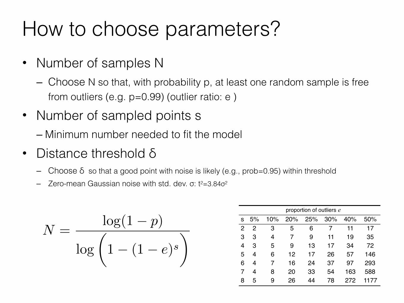
How to choose parameters?• Number of samples N – Choose N so that, with probability p, at least one random sample is free
from outliers (e.g. p=0.99) (outlier ratio: e )
• Number of sampled points s –Minimum number needed to fit the model
• Distance threshold δ – Choose δ so that a good point with noise is likely (e.g., prob=0.95) within threshold – Zero-mean Gaussian noise with std. dev. σ: t2=3.84σ2
proportion of outliers es 5% 10% 20% 25% 30% 40% 50%2 2 3 5 6 7 11 173 3 4 7 9 11 19 354 3 5 9 13 17 34 725 4 6 12 17 26 57 1466 4 7 16 24 37 97 2937 4 8 20 33 54 163 5888 5 9 26 44 78 272 1177
N =
log(1� p)
log
✓1� (1� e)s
◆

Good • Robust to outliers • Applicable for larger number of parameters than Hough transform • Parameters are easier to choose than Hough transform
Bad • Computational time grows quickly with fraction of outliers and
number of parameters • Not good for getting multiple fits
Common applications • Computing a homography (e.g., image stitching) • Estimating fundamental matrix (relating two views)

Given two images…
find matching features (e.g., SIFT)

Matched points will usually contain bad correspondences
good correspondence
bad correspondence
how should we estimate the transform?

LLS or DLT will find the ‘average’ transform
‘average’ transform
solution is corrupted by bad correspondences

Use RANSAC
How many correspondences to compute translation transform?

Need only one correspondence, to find translation model

Pick one correspondence, count inliers
onecorrespondence

Pick one correspondence, count inliers
2 inliers

Pick one correspondence, count inliers
onecorrespondence

Pick one correspondence, count inliers
5 inliers

Pick one correspondence, count inliers
5 inliers
Pick the model with the highest number of inliers!

Estimating homography using RANSAC
• RANSAC loop
1. Get four point correspondences (randomly)
2. Compute H (DLT)
3. Count inliers
4. Keep if largest number of inliers
• Recompute H using all inliers

Estimating homography using RANSAC
• RANSAC loop
1. Get four point correspondences (randomly)
2. Compute H using DLT
3. Count inliers
4. Keep if largest number of inliers
• Recompute H using all inliers

Estimating homography using RANSAC
• RANSAC loop
1. Get four point correspondences (randomly)
2. Compute H using DLT
3. Count inliers
4. Keep if largest number of inliers
• Recompute H using all inliers
Estimating homography using RANSAC
• RANSAC loop
1. Get four point correspondences (randomly)
2. Compute H using DLT
3. Count inliers
4. Keep H if largest number of inliers
• Recompute H using all inliers

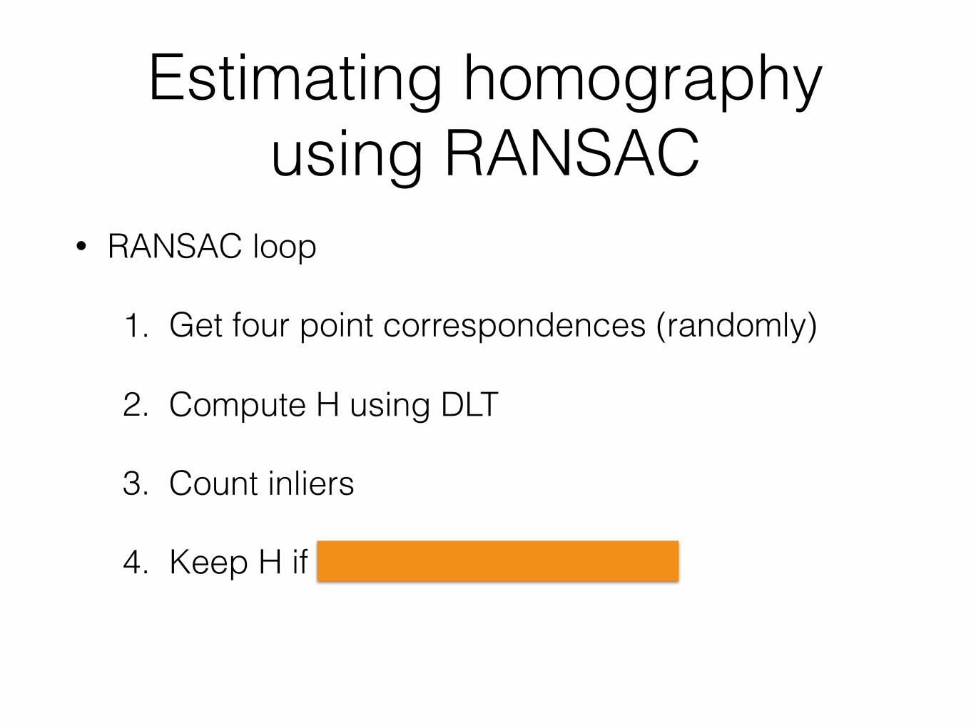
Estimating homography using RANSAC
• RANSAC loop
1. Get four point correspondences (randomly)
2. Compute H using DLT
3. Count inliers
4. Keep H if largest number of inliers
• Recompute H using all inliers

Useful for…