11. Bootstrap Methods

c A. Colin Cameron & Pravin K. Trivedi 2006

These transparencies were prepared in 20043.

They can be used as an adjunct to

Chapter 11 of our subsequent book

Microeconometrics: Methods and Applications

Cambridge University Press, 2005.

Original version of slides: May 2004

Bootstrap MethodsOutline

1. Introduction

2. Bootstrap Overview

3. Bootstrap Example

4. Bootstrap Theory

5. Bootstrap Extensions

6. Bootstrap Applications

1 Introduction

� Exact �nite sample results usually unavailable.Instead use asymptotic theory - limit normal and �2.

� Bootstrap due to Efron (1979) is an alternativemethod.Approximate distribution of statistic by Monte Carlosimulation, with sampling from the empirical distrib-ution or the �tted distribution of the observed data.

� Like conventional methods relies on asymptotic the-ory so only exact in in�nitely large samples.

� Simplest bootstraps no better than usual asymp-totics but may be easier to implement.

� More complicated bootstraps provide asymptoticre�nement so perhaps better �nite sample approx-imation.

2 Bootstrap Summary

� Sample: fw1; :::;wNg iid over iUsually: wi = (yi;xi)

� Estimator: b� is smooth root-N consistent and isasymptotically normal.Simplicity: state results for scalar �.

� Statistics of interest:

� estimate b�� standard errors sb�� t�statistic t = (b���0)=sb� where �0 isH0 value� associated critical value or p�value for the test

� con�dence interval.

2.1 Bootstrap Without Re�nement

� Estimate variance V[b�] of the sample meanb� = �y = N�1PNi=1 yi where yi is iid [�; �

2].

� Obtain S samples of size N from the population.Gives S estimates b�s = �ys, s = 1; :::; S.Then bV[b�] = (S � 1)�1PSs=1(b�s � b�)2,where b� = S�1PSs=1 b�s.

� This approach not possible as only have one sample.Bootstrap: treat the sample as the population.So �nite population is the actual data y1; :::; yN .Draw B bootstrap samples from this population ofsize N , sampling from y1; :::; yN with replacement.[In each bootstrap sample some original data pointsappear more than once while others appear at all.]Gives B estimates b�b = �yb, b = 1; :::; B.Then V[b�] = (B � 1)�1PBb=1(b�b � b�)2,where b� = B�1PBb=1 b�b.

2.1.1 Bootstrap Example

� Data generated from an exponential distribution withan exponential mean with two regressors

yijx2i; x3i � exponential(�i); i = 1; :::; 50�i = exp(�1 + �2x2i + �3x3i)

(x2i; x3i) � N [0:1; 0:1; 0:12; 0:12; 0:005](�1; �2; �3) = (�2; 2; 2):

� MLE for 50 observations gives b�1; b�2; b�3Focus on statistical inference for �3 :b�3 = 4:664 s3 = 1:741 t3 = 2:679.

� Use paired bootstrap with (yi; x2i; x3i) jointly re-sampled with replacement B = 999 times.

� Bootstrap standard error estimate = 1:939since b��3;1; :::; b��3;999 had mean 4:716 andstandard deviation of 1:939.

[compared to usual asymptotic estimate of 1:741).

2.2 Asymptotic Re�nements

� Example: Nonlinear estimators asymptotically unbi-ased but biased in �nite samples

� Often can show that

E[b� � �0] = aNN+bNN2

+cNN3

+ :::

where aN , bN and cN are bounded constants thatvary with the data and estimator.

� Consider alternative estimator e� withE[e� � �0] = BN

N2+CNN3

+ :::

where BN and CN are bounded constants.

� Both estimators are unbiased as N !1.The latter is an asymptotic re�nement:asymptotic bias of size O(N�2) < O(N�1).

� Bootstrap one of several asymptotic re�nement meth-ods.

� Smaller asymptotic bias not guaranteed to give smaller�nite sample bias:

BN=N2 > (aN=N + bN=N

2)

is possible for small N .

� Need simulation studies to con�rm �nite sample gains.

2.3 Asymptotically Pivotal Statistic

� Asymptotic re�nement for tests and conf. intervals.� = nominal size for a test, e.g. � = 0:05.Actual size= � + O(N�1=2) for usual one-sidedtests.

� Asymptotic re�nement requires statistic to be an as-ymptotically pivotal statistic, meaning limit distri-bution does not depend on unknown parameters.

� e.g. Sampling from yi � [�; �2].

� b� = �ya� N [�; �2=N ] is not asymptotically piv-

otal since distribution depends on unknown �2.

� t = (b� � �0)=sb� a� N [0; 1], the studentizedstatistic, is asymptotically pivotal.

� Estimators are usually not asymptotically pivotal.Conventional tests and CI�s are asymp. pivotal.

2.4 The Bootstrap

A general bootstrap algorithm is as follows:

1. Given data w1; :::;wNdraw a bootstrap sample of size N (see below)denote this new sample w�1; :::;w

�N .

2. Calculate an appropriate statistic using the bootstrapsample. Examples include:(a) estimate b�� of �;(b) standard error sb�� of estimate b��(c) t�statistic t� = (b�� � b�)=sb�� centered at b�.

3. Repeat steps 1-2 B independent times.GivesB bootstrap replications of b��1; :::; b��B or t�1; : : : ; t�Bor .....

4. Use these B bootstrap replications to obtain a boot-strapped version of the statistic (see below).

2.4.1 Bootstrap Sampling Methods (step 1)

� Empirical distribution function (EDF) bootstrapor nonparametric bootstrap.w�1; :::;w

�N obtained by sampling with replacement

from w1; :::;wN (used earlier).Also called paired bootstrap as for single equationmodels the pair (yi;xi) is being resampled.

� Parametric bootstrap for fully parametric models.Suppose yjx �F (x; �0) and have estimate b� p! �0.Bootstrap generate y�i by random draws from F (xi;

b�)where xi may be the original sample[or may �rst resample x�i from x1; :::;xN ]

� Residual bootstrap for additive error regressionSuppose yi = g(xi;�) + ui:Form �tted residuals bu1; :::; buN .Bootstrap residuals (bu�1; :::; bu�N) yield bootstrap sam-ple (y�1;x1); :::; (y

�N ;xN), for y

�i = g(xi;

b�) + bu�i .

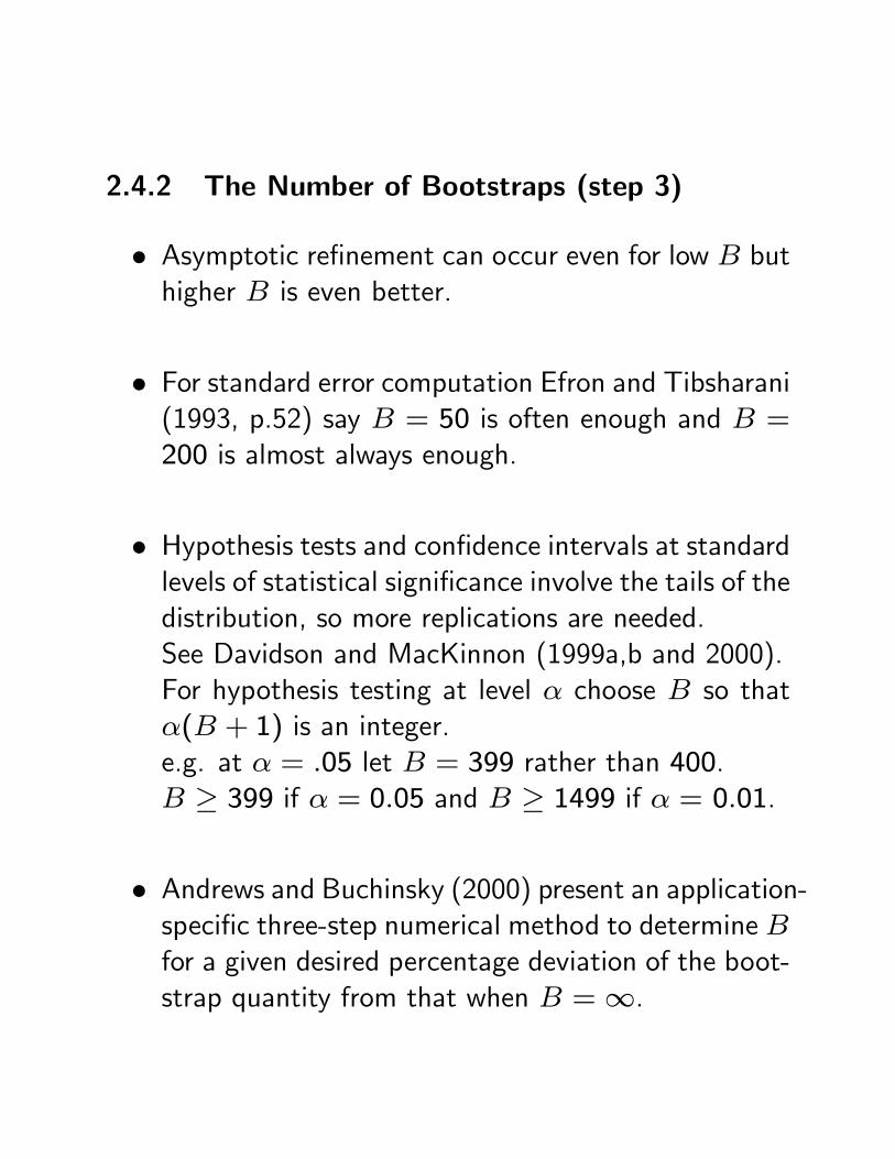
2.4.2 The Number of Bootstraps (step 3)

� Asymptotic re�nement can occur even for low B buthigher B is even better.

� For standard error computation Efron and Tibsharani(1993, p.52) say B = 50 is often enough and B =200 is almost always enough.

� Hypothesis tests and con�dence intervals at standardlevels of statistical signi�cance involve the tails of thedistribution, so more replications are needed.See Davidson and MacKinnon (1999a,b and 2000).For hypothesis testing at level � choose B so that�(B + 1) is an integer.e.g. at � = :05 let B = 399 rather than 400.B � 399 if � = 0:05 and B � 1499 if � = 0:01.

� Andrews and Buchinsky (2000) present an application-speci�c three-step numerical method to determine Bfor a given desired percentage deviation of the boot-strap quantity from that when B =1.

2.5 Standard Error Estimation

� The bootstrap estimate of variance of an estima-tor is the usual formula for estimating a variance,applied to the B bootstrap replications b��1; : : : ; b��B:

s2b�;Boot = 1

B � 1

BXb=1

(b��b � b��)2;where b�� = B�1PBb=1 b��b :

� The bootstrap estimate of the standard error,sb�;Boot, is obtained by taking the square root.

� This bootstrap provides no asymptotic re�nement.But extraordinarily useful when it is di¢ cult to obtainstandard errors using conventional methods:� Sequential two-step m-estimator� 2SLS estimator with heteroskedastic errors (if noWhite option).� Functions of other estimates e.g. b� = b�=b�� Clustered data with many small clusters, such asshort panels. Then resample the clusters.

2.6 Tests with Asymptotic Re�nement

� TN = (b�� �0)=sb� a� N [0; 1] is asymptotically piv-otal, so bootstrap this.

� Bootstrap gives B test statistics t�1; : : : ; t�B, where

t�b = (b��b � b�)=sb��b ;

is centered around the original estimate b� sinceresampling is from a distribution centered around b�.

� Let t�1; : : : ; t�B denote statistics ordered from small-est to largest.

� Upper alternative test: H0 : � � �0 vs Ha : � > �0the bootstrap critical value (at level �) is theupper � quantile of the B ordered test statistics.e.g. if B = 999 and � = 0:05 thenthe critical value is the 950th highest value of t�,since then (B + 1)(1� �) = 950.

� Can also compute a bootstrap p�value.e.g. if original statistic t lies between the 914th and915th largest values and B = 999 then pboot =1� 914=(B + 1) = 0:086.

� For a non-symmetrical test the bootstrap criticalvalues (at level �) are the lower �=2 and upper �=2quantiles of the ordered test statistics t�.Reject H0 if the original t lies outside this range.

� For a symmetrical test we instead order jt�j and thebootstrap critical value (at level �) is the upper �quantile of the ordered jt�j.Reject H0 if jtj exceeds this critical value.

� These tests, using the percentile-t method, provideasymptotic re�nements.One-sided t test and a non-symmetrical two-sided ttest the true size �+O(N�1=2)! �+O(N�1).Two-sided symmetrical t test or an asymptotic chi-square test true size �+O(N�1)! �+O(N�2).

2.6.1 Tests without Asymptotic Re�nement

� Alternative bootstrap methods can be used. Whileasymptotically valid there is no asymptotic re�ne-ment.

1. Compute t = (b���0)=sb�,boot where sb�,boot replacesthe usual estimate sb�.Compare this test statistic to standard normal criticalvalues.

2. For two-sided test of H0 : � = �0 against Ha : � 6=�0 �nd the lower �=2 and upper �=2 quantiles ofthe bootstrap estimates b��1; :::; b��B.Reject H0 if the original estimate b� follows outsidethis region.This is called the percentile method.

� These two bootstraps do not require computationof sb�, the usual standard error estimate based onasymptotic theory.

2.6.2 Bootstrap Example (continued)

� Summary statistics and percentiles based on 999 pairedbootstrap resamples for:(1) estimate b��3;(2) the associated statistics t�3 = (

b��3�4:664)=sb��3;(3) t(47) quantiles;(4) standard normal quantiles.

b��3 t�3 z=t(1) t(47)Mean 4.716 0.026 1.021 1.000

St.Dev. 1.939 1.047 1.000 1.0211% -.336 -2.664 -2.326 -2.408

2.5% 0.501 -2.183 -1.960 -2.0125% 1.545 -1.728 -1.645 -1.67825% 3.570 -0.621 -0.675 -0.68050% 4.772 0.062 0.000 0.00075% 5.971 0.703 0.675 0.68095% 7.811 1.706 1.645 1.678

97.5% 8.484 2.066 1.960 2.01299.0% 9.427 2.529 2.326 2.408

� Hypothesis Testing with Asymptotic Re�nement:Test H0 : �3 = 0 vs Ha : �3 6= 0 at level :05.Compute t�3 = (

b��3 � 4:664)=sb��3.Bootstrap critical values are �2:183 and 2:066.Reject H0 since original t3 = 2:679 > 2:066,

� Figure plots bootstrap estimate of the density of t3and compares it to the standard normal.

� Hypothesis Testing without Asymptotic Re�ne-ment 1:Use the bootstrap standard error estimate of 1:939,rather than the asymptotic standard error estimateof 1:741.Then t3 = (4:664� 0)=1:939 = 2:405.Reject H0 at level :05 as 2:405 > 1:960 using stan-dard normal critical values.

� Hypothesis Testing without Asymptotic Re�ne-ment 2:From Table 11.1, 95 percent of the bootstrap esti-mates b��3 lie in the range (0:501; 8:484):Reject H0 : �3 = 0 as this range does not includethe hypothesized value of 0.

2.7 Con�dence Intervals

� Statistics literature focuses on con�dence intervals.

� Asymptotic re�nement using the percentile-t method:The 100(1� �) percent con�dence interval is

(b� � t�[1��=2] � sb�; b� + t�[�=2] � sb�);where b� and sb� are the estimate and standard errorfrom the original sample andt�[1��=2] and t

�[�=2] denote the lower and upper �=2

quantiles �=2 of the t�statistics t�1; : : : ; t�B.

� The bias-corrected and accelerated (BCa) methoddetailed in Efron (1987) gives asymptotic re�nementfor a wider class of problems.

� No asymptotic re�nement (though valid).1. (b� � z[1��=2] � sb�;boot; b� + z[�=2] � sb�;boot)2. (b��[1��=2]; b��[�=2]) the percentile method.

2.8 Bias Reduction

� Most estimators are biased in �nite samples.We wish to estimate the bias E[b�]� �.

� Let b�� denote the average of b�� from the bootstraps.The bootstrap estimate of the bias is then

Biasb� = (b�� � b�):� If b� = 4 and b�� = 5 then b� overestimates by 1(truth was 4 and the many estimates averaged 5):So the bias-corrected estimate is 4� 1 = 3.

� The bootstrap bias-corrected estimator of � is

b�Boot = b� � (b�� � b�) = 2b� � b��:Note that b�� itself is not the bias-corrected estimate.The asymptotic bias of b�Boot is instead O(N�2).

� Bias correction is seldom used forpN consistent

estimators, as b�Boot can be more variable than b�and bias is often small relative to standard error.

2.8.1 Bootstrap Example (continued)

� Bootstrap: c�3� = 4:716Original estimate c�3 = 4:664.Estimated bias = (4:716� 4:664) = 0:052Bias-corrected estimate = 4:664� 0:052 = 4:612

� The bias of 0:052 is small compared to the standarderror s3 = 1:741.

3 Bootstrap in Stata

� * For exponential model MLE command is* ereg y x z

� * To bootstrapbs "ereg y x z" "_b[z]", reps(999) level(95)

Var Reps Observe Bias St.err. 95% CI_bs_1 999 4.663 .052 1.939 (.86,8.47) (N)

(.50,8.48) (P)(.23,8.17) (BC)

� N = normal is no re�nement method 1P = percentile is no re�nement method 2BC = bias-corrected is Efron (1986) re�nement

� Stata does not do the percentile-t method.But can save the 999 estimated coe¢ cients.Then use these to form 999 t-statistics, etc.

4 Bootstrap Theory

� See Horowitz (2001) - detailed though challenging.

� For root-N asymptotically normal statistic

� The bootstrap should be from distribution FNconsistent for the dgp F0.

� The bootstrap requires smoothness and continu-ity in F0 (the dgp) and GN (the �nite sampledistribution of the statistic).

� The bootstrap assumes existence of low ordermoments, as low order cumulants appear in theEdgeworth expansions that the bootstrap imple-ments.

� Asymptotic re�nement requires use of an asymp-totically pivotal statistic.

� Bootstrap re�nement presented assumes iid data.Care needed even for heteroskedastic errors.

5 Bootstrap Extensions

� 1-2 permit consistent bootstrap for a wider range ofapplications. 3-5 give asymptotic re�nement.

� 1. Subsample Bootstrap: bootstrap resampleof size m substantially smaller than sample sizeN . For nonsmooth estimators.

� 2. Moving blocks bootstrap: split sample intonon-overlapping blocks and sample with replace-ment from these blocks. For dependent data.

� 3. Nested bootstrap: bootstrap within a boot-strap.Provides asymptotic re�nement for t-test even ifdon�t have formula for standard error.

� 4. Recentering and Rescaling: Ensure boot-strap based on estimate that imposes all the con-ditions of the model under consideration. e.g.over-identi�ed GMM.

� 5. Jackknife: Precursor of the bootstrap.

6 Bootstrap Applications

1. Heteroskedastic Errors: For asymptotic re�nementuse the wild bootstrap.

2. Panel Data and Clustered Data: Resample allobservation in the cluster.e.g. For panel data (i; t) resample over i only.No re�nement but gives heteroscedasticity and panelrobust standard errors. on the cluster unit.

3. Hypothesis and Speci�cation Tests: consider morecomplicated tests.e.g. Can implement Hausman test without asymp-totic re�nement by bootstrap.e.g. can do bootstrap re�nement on LM tests thathave �poor �nite sample properties�

4. GMM and EL in Over-identi�ed Models: Foroveridenti�ed models need to recenter or use em-pirical likelihood.

5. Nonparametric Regression: Nonparametric den-sity and regression estimators converge at rate lessthan root-N and are asymptotically biased. Thiscomplicates inference such as con�dence intervals.Bootstrap works.

6. Non-Smooth Estimators: e.g. LAD.

7. Time Series: bootstrap residuals if possible or domoving blocks.

7 Some References

Andrews, D.W.K. and M. Buchinsky (2000), �A Three-step Method for choosing the Number of Bootstrap Repli-cations,�Econometrica, 68, 23-51.

Brownstone, D. and C. Kazimi (1998), �Applying theThe Bootstrap,�Unpublished manuscript, Department ofEconomics, University of California - Irvine.

Efron, B. (1979), �Bootstrap Methods: Another Look atthe Jackknife,�Annals of Statistics, 7, 1-26.

Efron, B. (1982), �Better Bootstrap Con�dence Inter-vals,� Journal of the American Statistical Association,82, 171-185.

Efron, B. and J. Tibsharani (1993), An Introduction tothe Bootstrap, London: Chapman and Hall.

Hall, P. and J.L Horowitz (1996), �Bootstrap critical val-ues for tests based on Generalized Method of MomentsEstimators,�Econometrica, 64, 891-916.

Horowitz, J.L. (1994), �Bootstrap-based Critical Valuesfor the Information Matrix Test,� Journal of Economet-rics, 61, 395-411.

Horowitz, J.L. (2001), �The Bootstrap,� Handbook ofEconometrics: Volume 5, Amsterdam: North-Holland.