1.1 First Things 1.2 Introduction

Spectral Graph Theory Lecture 1

Introduction

Daniel A. Spielman August 29, 2018

1.1 First Things

1. Please call me “Dan”. If such informality makes you uncomfortable, you can try “ProfessorDan”. If that fails, I will also answer to “Prof. Spielman”.

2. If you are going to take this course, please sign up for it on Canvas. This is the only way youwill get emails like “Problem 3 was false, so you don’t have to solve it”.

3. This class meets this coming Friday, September 31, but not on Labor Day, which is Monday,September 3.

1.2 Introduction

I have three objectives in this lecture: to give you an overview of the material we will cover thissemester, to help you decide if this course is right for you, and to tell you how the course will work.

As the title suggests, this course is about the eigenvalues and eigenvectors of matrices associatedwith graphs, and their applications. I will never forget my amazement at learning that combinatorialproperties of graphs could be revealed by an examination of the eigenvalues and eigenvectors oftheir associated matrices. I hope to both convey my amazement to you and to make it feel likecommon sense. I’m now shocked when any important property of a graph is not revealed by itseigenvalues and eigenvectors.

This class will fundamentally be a math class, and my emphasis is on material that I find beautifuland/or useful. I’ll present a lot of theorems, a few algorithms, and a bunch of open problems.

1.3 Mechanics

There is no book for this course, but I will produce notes for every lecture. You should readthe lecture notes. They will often contain material that I did not have time to cover in class.They will sometimes contain extra expositions of elementary topics. I will try to make the notesavailable before lecture. Some students will want to print them out for reference during lecture.

Given that I am providing lecture notes, you might not need to take notes during lecture. I,however, take notes during every lecture that I attend. It helps me pay attention and rememberwhat is going on. But, there are many different learning styles. You may prefer to just listen.

1-1

Lecture 1: August 29, 2018 1-2

If you would like a book that covers some of the material from the course, I suggest one of

“Algebraic Graph Theory” by Chris Godsil and Gordon Royle,

“Spectral Graph Theory” by Fan Chung, or

“Algebraic Combinatorics” by Chris Godsil.

I expect to produce around 5 or 6 problem sets during the semester. Some of the problems I assignin these will be very hard. You will be allowed to work on them in small groups.

For some lectures, such as today’s, I have assigned a number of “exercises” at the end of the lecturenotes. You should solve these on your own, as soon after lecture as possible. You should nothand them in. They are just to help you practice the material. Today’s exercises are a review offundamental linear algebra. I will put the solutions to some of them on Canvas.

There will be no tests or exams.

1.3.1 This is a graduate course

As some undergrads are thinking about taking this course, I thought I should explain the maindifferences between an undergraduate course and a graduate course, and the differences in outlookbetween undergrads and graduate students.

Graduate school is essentially pass/fail. Graduate students either write a thesis and graduate, orthey do not. Their grades in courses do not matter very much. Most are here because they thinkthey might learn something in this course that they will find useful in their careers. This meansthat some of them will work very hard.

Graduate students are also occasionally occupied with other responsibilities, like teaching andresearch. For this reason, I will give students at least two weeks to complete the problems I assign.However, I recommend that you solve the easier problems immediately.

Graduate students routinely take courses for which they do not have all the prerequisite knowledge.I assume that they can learn anything elementary as needed. Wikipedia makes this much easierthan it used to be.

Finally, graduate courses are not as “user friendly” as undergraduate courses. I make no guaranteesabout what will happen in this course. I may assign more or fewer problem sets than I haveannounced. I may completely change the topics that I decide to cover. You have been warned.

1.3.2 Other courses

I have adjusted my selection of material for this course to decrease overlap with others. For example,I am omitting some material that will be included in S&DS 684a: Statistical Inference on Graphsand S&DS 615b: Introduction to Random Matrix Theory.


1.4 Background: Graphs

First, we recall that a graph G = (V,E) is specified by its vertex1 set, V , and edge set E. In anundirected graph, the edge set is a set of unordered pairs of vertices. Unless otherwise specified, allgraphs will be undirected, simple (having no loops or multiple edges) and finite. We will sometimesassign weights to edges. These will usually be real numbers. If no weights have been specified, weview all edges as having weight 1. This is an arbitrary choice, and we should remember that it hasan impact.

Graphs (also called “networks”) are typically used to model connections or relations between things,where “things” are vertices. However, I often prefer to think of the edges in a graph as being moreimportant than the vertices. In this case, I may just specify an edge set E, and ignore the ambientvertex set.

Common “natural” examples of graphs are:

• Friendship graphs: people are vertices, edges exist between pairs of people who are friends(assuming the relation is symmetric).

• Network graphs: devices, routers and computers are vertices, edges exist between pairs thatare connected.

• Circuit graphs: electronic components, such as transistors, are vertices: edges exist betweenpairs connected by wires.

• Protein-Protein Interaction graphs: proteins are vertices. Edges exist between pairs thatinteract. These should really have weights indicating the strength and nature of interaction.Most other graphs should to.

It is much easier to study abstract, mathematically defined graphs. For example,

• The path on n vertices. The vertices are {1, . . . n}. The edges are (i, i+ 1) for 1 ≤ i < n.

• The ring on n vertices. The vertices are {1, . . . n}. The edges are all those in the path, plusthe edge (1, n).

• The hypercube on 2k vertices. The vertices are elements of {0, 1}k. Edges exist betweenvertices that differ in only one coordinate.

1.5 Matrices for Graphs

The naive view of a matrix is that it is essentially a spreadsheet—a table we use to organizenumbers. This is like saying that a car is an enclosed metal chair with wheels. It says nothingabout what it does!

1I will use the words “vertex” and “node” interchangeably. Sorry about that.


I will use matrices to do two things. First, I will view a matrix M as providing an function thatmaps a vector x to the vector M x . That is, I view M as an operator. Second, I view a matrixM as providing a function that maps a vector x to a number xTM x . That is, I use M to definea quadratic form.

1.5.1 A spreadsheet

We will usually write V for the set of vertices of a graph, and let n denote the number of vertices.There are times that we will need to order the vertices and assign numbers to them. In this case,they will usually be {1, . . . , n}. For example, if we wish to draw a matrix as a table, then we needto decide which vertex corresponds to which row and column.

The most natural matrix to associate with a graph G is its adjacency matrix2, M G, whose entriesM G(a, b) are given by

M G(a, b) =

{1 if (a, b) ∈ E0 otherwise.

It is important to observe that I index the rows and columns of the matrix by vertices, rather thanby number. Almost every statement that we make in this class will remain true under renamingof vertices. The first row of a matrix has no special importance. To understand this better see theexercises at the end of the lecture.

While the adjacency matrix is the most natural matrix to associate with a graph, I also find it theleast useful. Eigenvalues and eigenvectors are most meaningful when used to understand a naturaloperator or a natural quadratic form. The adjacency matrix provides neither.

1.5.2 An operator

The most natural operator associated with a graph G is probably its diffusion operator. Thisoperator describes the diffusion of stuff among the vertices of a graph and how random walksbehave. We will save further discussion of this perspective for a later lecture.

1.5.3 A quadratic form

The most natural quadratic form associated with a graph is defined in terms of its Laplacian matrix,

LGdef= DG −M G,

where DG is the diagonal matrix in which DG(a, a) is the degree of vertex a. We will usually writed(a) for the degree of vertex a. In an unweighted graph, the degree of a vertex is the number ofedges attached to it. In the case of a weighted graph, we use the weighted degree: the sum of theweights of the edges attached to the vertex a.

2I am going to try to always use the letter M for the adjacency matrix, in contrast with my past practice whichwas to use A. I will use letter like a and b to denote vertices.


Given a function on the vertices, x ∈ IRV , the Laplacian quadratic form is

xTLGx =∑

(a,b)∈E

(x (a)− x (b))2. (1.1)

This form measures the smoothness of the function x . It will be small if the function x does notjump too much over any edge.

I use the notation x (a) to denote the coordinate of vector x corresponding to vertex a. Otherpeople often use subscripts for this, like x a. I reserve subscripts for other purposes.

1.6 Background: Spectral Theory

I now review the highlights of the spectral theory for symmetric matrices. Almost all of the matriceswe consider in this course will be symmetric or will be similar3 to symmetric matrices.

We recall that a vector ψ is an eigenvector of a matrix M with eigenvalue λ if

Mψ = λψ. (1.2)

That is, λ is an eigenvalue if and only if λI −M is a singular matrix. Thus, the eigenvalues arethe roots of the characteristic polynomial of M :

det(xI −M ).

Theorem 1.6.1. [The Spectral Theorem] If M is an n-by-n, real, symmetric matrix, then thereexist real numbers λ1, . . . , λn and n mutually orthogonal unit vectors ψ1, . . . ,ψn and such that ψi

is an eigenvector of M of eigenvalue λi, for each i.

This is the great fact about symmetric matrices. If the matrix is not symmetric, it might not haven eigenvalues. And, even if it has n eigenvalues, their eigenvectors will not be orthogonal4. In fact,if M is not symmetric, then its eigenvalues and eigenvalues might be the wrong thing to look at.

I remind you that the eigenvectors are not uniquely determined, although the eigenvalues are. Ifψ is an eigenvector, then −ψ is as well. Some eigenvalues can be repeated. If λi = λi+1, thenψi + ψi+1 will also be an eigenvector of eigenvalue λi. Generally, the eigenvectors of a giveneigenvalue are only determined up to an orthogonal transformation.

Fact 1.6.2. The Laplacian matrix of a graph is positive semidefinite. That is, all its eigenvaluesare nonnegative.

Proof. Let ψ be a unit eigenvector of L of eigenvalue λ. Then,

ψTLψ = ψTλψ = λ =∑

(a,b)∈E

(ψ(a)−ψ(b))2 > 0.

3A matrix M is similar to a matrix B if there is a non-singular matrix X such that X−1M X = B . In this case,M and B have the same eigenvalues. See the exercises at the end of this lecture.

4You can prove that if the eigenvectors are orthogonal, then the matrix is symmetric.


We always number the eigenvalues of the Laplacian from smallest to largest. Thus, λ1 = 0. Wewill refer to λ2, and in general λk for small k, as low-frequency eigenvalues. λn is a high-frequencyeigenvalue. We will see why in a moment.

1.7 Overview of the course

We will begin the course by learning about the eigenvalues and eigenvectors of many special graphs.These will include simple graphs like paths, rings, stars, trees and hypercubes, and we will eventuallyget to Cayley graphs and Strongly Regular Graphs.

Before we get to any theorems, I would like to convince you that the eigenvalues and eigenvectorsof graphs are meaningful by showing you some examples. I will do these examples in Julia usinga Jupyter notebook. I include snippets of the code and the images they generate in this text, andhave provided the notebook on the course webpage.

1.7.1 Paths

A path graph has vertices {1, . . . , n} and edges (i, i+1) for 1 ≤ i < n. Here is the adjacency matrixof a path graph on 4 vertices.

M = path_graph(4)

Matrix(M)

0.0 1.0 0.0 0.0

1.0 0.0 1.0 0.0

0.0 1.0 0.0 1.0

0.0 0.0 1.0 0.0

And, here is its Laplacian matrix

Matrix(lap(M))

1.0 -1.0 0.0 0.0

-1.0 2.0 -1.0 0.0

0.0 -1.0 2.0 -1.0

0.0 0.0 -1.0 1.0

Here are the eigenvalues of a longer path.

L = lap(path_graph(10))

E = eigen(Matrix(L))

println(E.values)

[0.0, 0.097887, 0.381966, 0.824429, 1.38197, 2.0, 2.61803, 3.17557, 3.61803, 3.90211]


The eigenvector of the zero-eigenvalue is a constant vector (up to numerical issues):

E.vectors[:,1]

0.31622776601683755

0.31622776601683716

0.31622776601683766

0.3162277660168381

0.31622776601683855

0.3162277660168381

0.3162277660168385

0.31622776601683805

0.3162277660168378

0.3162277660168378

The eigenvector of λ2 is the lowest frequency eigenvector, as we can see that it increases monoton-ically along the path:

v2 = E.vectors[:,2]

-0.44170765403093937

-0.39847023129620024

-0.316227766016838

-0.20303072371134553

-0.06995961957075425

0.06995961957075386

0.2030307237113457

0.31622776601683766

0.3984702312961997

0.4417076540309382

Let’s plot that.


2 4 6 8 10

-0.4

-0.2

0.0

0.2

0.4

vertex number

valu

e in

eig

enve

ctor

plot(v2,marker=5,legend=false)

xlabel!("vertex number")

ylabel!("value in eigenvector")

The x-axis is the name/number of the vertex, and the y-axis is the value of the eigenvector at thatvertex. Now, let’s look at the next few eigenvectors.

2 4 6 8 10

-0.4

-0.2

0.0

0.2

0.4

Vertex Number

Val

ue in

Eig

enve

ctor

v2v3v4

Plots.plot(E.vectors[:,2],label="v2",marker = 5)

Plots.plot!(E.vectors[:,3],label="v3",marker = 5)


xlabel!("Vertex Number")

ylabel!("Value in Eigenvector")

You may now understand why I refer to these as the low-frequency eigenvectors. The curvesthey trace out resemble the low-frequency modes of vibration of a string. The reason for this is


that the path graph can be viewed as a discretization of the string, and its Laplacian matrix is adiscretization of the Laplace operator. We will relate the low-frequency eigenvalues to connectivity.

In contrast, the highest frequency eigenvalue alternates positive and negative with every vertex.We will show that these may be related to problems of graph coloring and finding independent sets.

2 4 6 8 10

-0.4

-0.2

0.0

0.2

0.4

Vertex Number

Val

ue in

Eig

enve

ctor

v10

Plots.plot(E.vectors[:,10],label="v10",marker=5)



1.7.2 Spectral Graph Drawing

We can often use the low-frequency eigenvalues to obtain a nice drawing of a graph. For example,here is 3-by-4 grid graph, and its first two non-trivial eigenvectors. Looking at them suggests thatthey might provide nice coordinates for the vertices.

M = grid2(3,4)

L = lap(M)


V = E.vectors[:,2:3]

-0.377172 0.353553

-0.15623 0.353553

0.15623 0.353553

0.377172 0.353553

-0.377172 -1.66533e-16

-0.15623 -4.16334e-16

0.15623 -5.82867e-16

0.377172 2.77556e-16


-0.377172 -0.353553

-0.15623 -0.353553

0.15623 -0.353553

0.377172 -0.353553

In the figure below, we use these eigenvectors to draw the graph. Vertex a be been plotted atcoordinates ψ2(a),ψ3(a). That is, we use ψ2 to provide a horizontal coordinate for every vertex,and ψ3 to obtain a vertical coordinate. We then draw the edges as straight lines.

plot_graph(M,V[:,1],V[:,2])

Let’s do a fancier example that should convince you something interesting is going on. I begin bygenerating points by sampling them from the Yale logo.


1.00 1.25 1.50 1.75 2.001.00

1.25

1.50

1.75

2.00

@load "yale.jld2"

scatter(xy[:,1],xy[:,2],legend=false)

I then construct a graph on them by forming their Delaunay triangulation. I won’t get to teachabout Delaunay triangulations during this course. But, they are terrific and I recommend that youlook them up.

Since the vertices came with coordinates, it was easy to draw a nice picture of the graph. But, whatif we just knew the graph, and not the coordinates? We could generate coordinates by computingtwo eigenvectors, and using each as a coordinate. Below, I plot vertex a at position ψ2(a),ψ3(a),and again draw the edges as straight lines.

plot_graph(a,xy[:,1],xy[:,2])


plot_graph(a, v2,v3, dots=false)

That’s a great way to draw a graph if you start out knowing nothing about it. It’s the first thing Ido whenever I meet a strange graph. Note that the middle of the picture is almost planar, althoughedges do cross near the boundaries.

1.7.3 Graph Isomorphism

It is important to note that the eigenvalues do not change if we relabel the vertices. Moreover, if wepermute the vertices then the eigenvectors are similarly permuted. That is, if P is a permutationmatrix, then

Lψ = λψ if and only if (PLPT )(Pψ) = λ(Pψ),

because PTP = I . To prove it by experiment, let’s randomly permute the vertices, and plot thepermuted graph.


Random.seed!(1)

p = randperm(size(a,1))

M = a[p,p]

E = eigen(Matrix(lap(M)))

V = E.vectors[:,2:3]

plot_graph(M,V[:,1],V[:,2], dots=false)

Note that this picture is slightly different from the previous one: it has flipped vertically. That’sbecause eigenvectors are only determined up to signs, and that’s only if they have multiplicity 1.This gives us a very powerful heuristic for testing if one graph is a permutation of another (this isthe famous “Graph Isomorphism Testing Problem”). First, check if the two graphs have the samesets of eigenvalues. If they don’t, then they are not isomorphic. If they do, and the eigenvalueshave multiplicity one, then draw the pictures above. If the pictures are the same, up to horizontalor vertical flips, and no vertex is mapped to the same location as another, then by lining up thepictures we can recover the permutation.

As some vertices can map to the same location, this heuristic doesn’t always work. We will learnabout it to the extent to which it does. In particular, we will see that if every eigenvalue of twographs G and H have multiplicity 1, then we can efficiently test whether or not they are isomorphic.

These algorithms have been extended to handle graph in which the multiplicity of every eigenvalueis bounded by a constant. But, there are graphs in which every non-trivial eigenvalue has largemultiplicity. We will learn how to construct and analyze these, as they constitute fundamentalexamples and counter-examples to many natural conjectures. For example, here are the eigenvaluesof a Latin Square Graph on 25 vertices. These are a type of Strongly Regular Graph.

M = latin_square_graph(5);

println(eigvals(Matrix(lap(M))))

[0.0, 10.0, 10.0, 10.0, 10.0, 10.0, 10.0, 10.0, 10.0, 10.0, 10.0, 10.0, 10.0, 15.0, 15.0, 15.0, 15.0, 15.0, 15.0, 15.0, 15.0, 15.0, 15.0, 15.0, 15.0]


All Latin Square Graphs of the same size have the same eigenvalues, whether or not they areisomorphic. We will learn some surprisingly fast (but still not polynomial time) algorithms forchecking whether or not Strongly Regular Graphs are isomorphic.

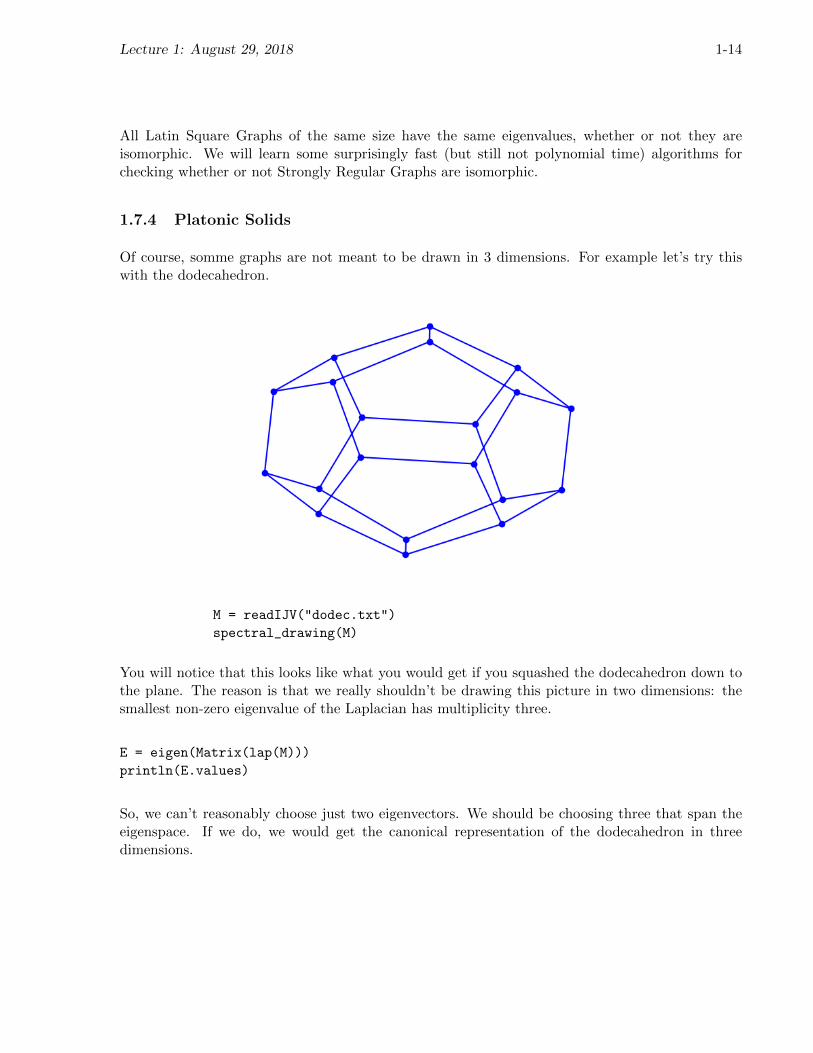
1.7.4 Platonic Solids

Of course, somme graphs are not meant to be drawn in 3 dimensions. For example let’s try thiswith the dodecahedron.

M = readIJV("dodec.txt")

spectral_drawing(M)

You will notice that this looks like what you would get if you squashed the dodecahedron down tothe plane. The reason is that we really shouldn’t be drawing this picture in two dimensions: thesmallest non-zero eigenvalue of the Laplacian has multiplicity three.

E = eigen(Matrix(lap(M)))

println(E.values)

So, we can’t reasonably choose just two eigenvectors. We should be choosing three that span theeigenspace. If we do, we would get the canonical representation of the dodecahedron in threedimensions.


x = E.vectors[:,2]

y = E.vectors[:,3]

z = E.vectors[:,4]

pygui(true)

plot_graph(M, x, y, z; setaxis=false)

As you would guess, this happens for all Platonic solids. In fact, if you properly re-weight the edges,it happens for every graph that is the one-skeleton of a convex polytope. Let me state that moreconcretely. A weighted graph is a graph along with a weight function, w, mapping every edge to apositive number. The adjacency matrix of a weighted graph has the weights of edges as its entries,instead of 1s. The diagonal degree matrix of a weighted graph, DG, has the weighted degrees onits diagonal. That is,

DG(i, i) =∑

j:(i,j)∈E

w(i, j).

The Laplacian then becomes LG = DG − AG. Given a convex polytope in IRd, we can treat its1-skeleton as a graph on its vertices. We will prove that there is a way of assigning weights to edgesso that the second-smallest Laplacian eigenvalue has multiplicity d, and so that the correspondingeigenspace is spanned by the coordinate vectors of the vertices of the polytope.

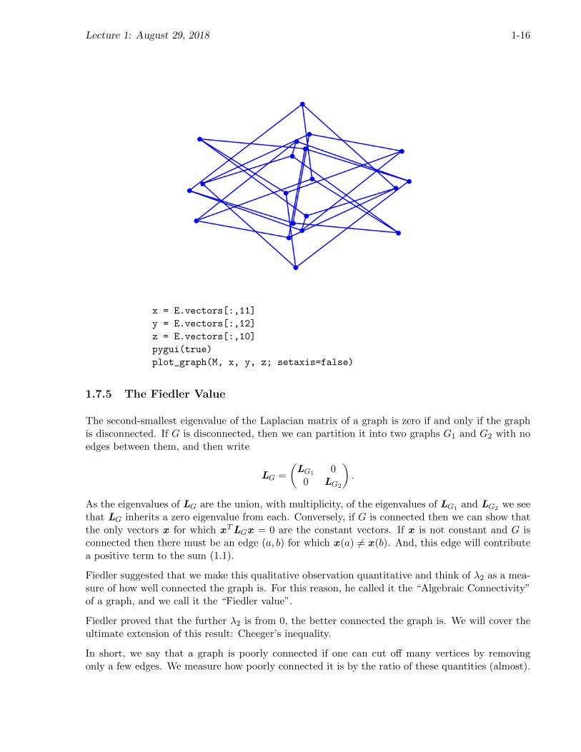
Before we turn off the computer, let’s take a look at the high-frequency eigenvectors of the dodec-ahedron.


x = E.vectors[:,11]

y = E.vectors[:,12]

z = E.vectors[:,10]

pygui(true)

plot_graph(M, x, y, z; setaxis=false)

1.7.5 The Fiedler Value

The second-smallest eigenvalue of the Laplacian matrix of a graph is zero if and only if the graphis disconnected. If G is disconnected, then we can partition it into two graphs G1 and G2 with noedges between them, and then write

LG =

(LG1 0

0 LG2

).

As the eigenvalues of LG are the union, with multiplicity, of the eigenvalues of LG1 and LG2 we seethat LG inherits a zero eigenvalue from each. Conversely, if G is connected then we can show thatthe only vectors x for which xTLGx = 0 are the constant vectors. If x is not constant and G isconnected then there must be an edge (a, b) for which x (a) 6= x (b). And, this edge will contributea positive term to the sum (1.1).

Fiedler suggested that we make this qualitative observation quantitative and think of λ2 as a mea-sure of how well connected the graph is. For this reason, he called it the “Algebraic Connectivity”of a graph, and we call it the “Fiedler value”.

Fiedler proved that the further λ2 is from 0, the better connected the graph is. We will cover theultimate extension of this result: Cheeger’s inequality.

In short, we say that a graph is poorly connected if one can cut off many vertices by removingonly a few edges. We measure how poorly connected it is by the ratio of these quantities (almost).


Cheeger’s inequality gives a tight connection between this ratio and λ2. If λ2 is small, then forsome t, the set of vertices

Sidef= {i : v2(i) < t}

may be removed by cutting much less than |Si| edges. This spectral graph partitioning heuristichas proved very successful in practice.

In general, it will be interesting to turn qualitative statements like this into quantitative ones. Forexample, we will see that the smallest eigenvalue of the diffusion matrix is zero if and only if thegraph is bipartite. One can relate the magnitude of this eigenvalue to how far a graph is from beingbipartite.

1.7.6 Bounding Eigenvalues

We will often be interested in the magnitudes of certain eigenvalues. For this reason, we will learnmultiple techniques for proving bounds on eigenvalues. The most prominent of these will be proofsby test vectors and proofs by comparison with simpler graphs.

1.7.7 Planar Graphs

We will prove that graphs that can be drawn nicely must have small Fiedler value, and we willprove very tight results for planar graphs.

We will also see how to use the graph Laplacian to draw planar graphs: Tutte proved that if onereasonably fixes the locations of the vertices on a face of a planar graph and then lets the otherssettle into the positions obtained by treating the edges as springs, then one obtains a planar drawingof the graph!

1.7.8 Random Walks on Graphs

Spectral graph theory is one of the main tools we use for analyzing random walks on graphs. Wewill spend a few lecture on this theory, connect it to Cheeger’s inequality, and use tools developedto study random walks to derive a fascinating proof of Cheeger’s inequality.

1.7.9 Expanders

We will be particularly interested in graphs that are very well connected. These are called expanders.Roughly speaking, expanders are sparse graphs (say a number of edges linear in the number ofvertices), in which λ2 is bounded away from zero by a constant. They are among the most importantexamples of graphs, and play a prominent role in Theoretical Computer Science.

Expander graphs have numerous applications. We will see how to use random walks on expandergraphs to construct pseudo-random generators about which one can actually prove something. Wewill also use them to construct good error-correcting codes.


Error-correcting codes and expander graphs are both fundamental objects of study in the field ofExtremal Combinatorics and are extremely useful. If students in the class have not learned aboutthese, I will teach about them. We will also use error-correcting codes to construct crude expandergraphs.

We will learn at least one construction of good expanders. The best expanders are the Ramanujangraphs. These were first constructed by Margulis and Lubotzky, Phillips and Sarnak. We mightfinish the class by proving the existence of Ramanujan graphs.

1.7.10 Approximations of Graphs

We will ask what it means for one graph to approximate another. Given graphs G and H, we willmeasure how well G approximates H by the closeness of their Laplacian quadratic forms. We willsee that expanders are precisely the sparse graphs that provide good approximations of the completegraph, and we will use this perspective for most of our analysis of expanders. We will show thatevery graph can be well-approximated by a sparse graph through a process called sparsification.

1.7.11 Solving equations in and computing eigenvalues of Laplacians

We will also ask how well a graph can be approximated by a tree, and see that low-stretch spanning-trees provide good approximations under this measure.

My motivation for this material is not purely graph-theoretic. Rather, it is inspired by the needto design fast algorithms for computing eigenvectors of Laplacian matrices and for solving linearequations in Laplacian matrices. This later problem arises in numerous contexts, including thesolution of elliptic PDEs by the finite element method, the solution of network flow problems byinterior point algorithms, and in classification problems in Machine Learning.

In fact, our definition of graph approximation is designed to suit the needs of the PreconditionedConjugate Gradient algorithm. We may finish the semester by learning how these algorithms work.

1.8 Eigenvalues and Optimization

One of the reasons that the eigenvalues of matrices have meaning is that they arise as the solutionto natural optimization problems. We will spend a lot of time on this connection next lecture. Fornow, we start with one result in this direction. Observe that its proof does not require the spectraltheorem.

Theorem 1.8.1. Let M be a symmetric matrix and let x be a non-zero vector that maximizes theRayleigh quotient with respect to M :

xTM x

xTx.

Then, x is an eigenvector of M with eigenvalue equal to the Rayleigh quotient. Moreover, thiseigenvalue is the largest eigenvalue of M .


Proof. We first observe that the maximum is achieved: As the Rayleigh quotient is homogeneous,it suffices to consider unit vectors x . As the set of unit vectors is a closed and compact set, themaximum is achieved on this set.

Now, let x be a non-zero vector that maximizes the Rayleigh quotient. We recall that the gradientof a function at its maximum must be the zero vector. Let’s compute that gradient.

We have∇xTx = 2x ,

and∇xTM x = 2M x .

So,

∇xTM x

xTx=

(xTx )(2M x )− (xTM x )(2x )

(xTx )2.

In order for this to be zero, we must have

M x =xTM x

xTxx .

That is, if and only if x is an eigenvector of M with eigenvalue equal to its Rayleigh quotient.

1.9 Exercises

The following exercises are for your own practice. They are intended as a review of fundamentallinear algebra. I have put the solutions in a separate file that you can find on Classes V2. Irecommend that you try to solve all of these before you look at the solutions, so that you can getback in practice at doing linear algebra.

1. Orthogonal eigenvectors. Let M be a symmetric matrix, and let ψ and φ be vectors so that

Mψ = µψ and Mφ = νφ.

Prove that if µ 6= ν then ψ must be orthogonal to φ. Note that your proof should exploit thesymmetry of M , as this statement is false otherwise.

2. Invariance under permutations.

Let Π be a permutation matrix. That is, there is a permutation π : V → V so that

Π(u, v) =

{1 if u = π(v), and

0 otherwise.

Prove that ifMψ = λψ,

then (ΠM ΠT

)(Πψ) = λ(Πψ).


That is, permuting the coordinates of the matrix merely permutes the coordinates of the eigenvec-tors, and does not change the eigenvalues.

3. Invariance under rotations.

Let Q be an orthonormal matrix. That is, a matrix such that QTQ = I . Prove that if

Mψ = λψ,

then (QM QT

)(Qψ) = λ(Qψ).

4. Similar Matrices.

A matrix M is similar to a matrix B if there is a non-singular matrix X such that X−1M X = B .Prove that similar matrices have the same eigenvalues.

5. Spectral decomposition.

Let M be a symmetric matrix with eigenvalues λ1, . . . , λn and let ψ1, . . . ,ψn be a correspondingset of orthonormal column eigenvectors. Let Ψ be the orthonormal matrix whose ith column isψi. Prove that

ΨTM Ψ = Λ,

where Λ is the diagonal matrix with λ1, . . . , λn on its diagonal. Conclude that

M = ΨΛΨT =∑i∈V

λiψiψTi .


Essential spectral theory, Hall’s spectral graph drawing, the Fiedler value

Daniel A. Spielman August 31, 2018

2.1 Eigenvalues and Optimization

The Rayleigh quotient of a vector x with respect to a matrix M is defined to be

xTMx

xTx.

At the end of the last class, I gave the following characterization of the largest eigenvalue of asymmetric matrix in terms of the Rayleigh quotient.

Theorem 2.1.1. Let M be a symmetric matrix and let x be a non-zero vector that maximizes theRayleigh quotient with respect to M :

xTMx

xTx.

Then, x is an eigenvector of M with eigenvalue equal to the Rayleigh quotient. Moreover, thiseigenvalue is the largest eigenvalue of M .

Proof. We first observe that the maximum is achieved: As the Rayleigh quotient is homogeneous,it suffices to consider unit vectors x . As the set of unit vectors is a closed and compact set, themaximum is achieved on this set.

Now, let x be a non-zero vector that maximizes the Rayleigh quotient. We recall that the gradientof a function at its maximum must be the zero vector. Let’s compute that gradient.

We have∇xTx = 2x ,

and∇xTMx = 2Mx .

So,

∇xTMx

xTx=

(xTx )(2Mx )− (xTMx )(2x )

(xTx )2.

In order for this to be zero, we must have

Mx =xTMx

xTxx .

That is, if and only if x is an eigenvector of M with eigenvalue equal to its Rayleigh quotient.

2-1


Of course, the analogous characterization holds for the smallest eigenvalue. A substantial general-ization of these characterizations is given by the Courant-Fischer Theorem. We will state it for theLaplacian, as that is the case we will consider for the rest of the lecture.

Theorem 2.1.2 (Courant-Fischer Theorem). Let L be a symmetric matrix with eigenvalues λ1 ≤λ2 ≤ · · · ≤ λn. Then,

λk = minS⊆IRn

dim(S)=k

maxx∈S

xTLx

xTx= max

T⊆IRn

dim(T )=n−k+1

minx∈T

xTLx

xTx.

For example, consier the case k = 1. In this case, S is just the span of ψ1 and T is all of IRn. Forgeneral k, the proof reveals that the optimum is achieved when S is the span of ψ1, . . . ,ψk andwhen T is the span of ψk, . . . ,ψn.

As many proofs in Spectral Graph Theory begin by expanding a vector in the eigenbasis of a matrix,we being by carefully stating a key property of these expansions.

Lemma 2.1.3. Let M be a symmetric matrix with eigenvalues µ1, . . . , µn and a correspondingorthnormal basis of eigenvectors ψ1, . . . ,ψn. Let x be a vector and expand x in the eigenbasis as

x =n∑

i=1

ciψi.

Then,

xTMx =

n∑i=1

c2iλi.

You should check for yourself (or recall) that ci = xTψi (this is obvious if you consider the standardcoordinate basis).

Proof. Compute:

xTMx =

(∑i

ciψi

)T

M

∑j

cjψj

=

(∑i

ciψi

)T∑

j

cjλjψj

=∑i,j

cicjλjψTi ψj

=∑i

c2iλi,

as ψTi ψj = 0 for i 6= j.


Proof of 2.1.2. Letψ1, . . . ,ψn be an orthonormal set of eigenvectors of L corresponding to λ1, . . . , λn.We will just verify the first characterization of λk. The other is similar.

First, let’s verify that λk is achievable. Let Sk be the span of ψ1, . . . ,ψk. We can expand everyx ∈ Sk as

x =k∑

i=1

ciψi.

Applying Lemma 2.1.3 we obtain

xTLx

xTx=

∑ki=1 λic

2i∑k

i=1 c2i

≤∑k

i=1 λkc2i∑k

i=1 c2i

= λk.

To show that this is in fact the maximum, we will prove that for all subspaces S of dimension k,

maxx∈S

xTLx

xTx≥ λk.

Let Tk be the span of ψk, . . . ,ψn. As Tk has dimension n− k + 1, every S of dimension k has anintersection with Tk of dimension at least 1. So,

maxx∈S

xTLx

xTx≥ max

x∈S∩Tk

xTLx

xTx.

Any such x may be expressed as

x =n∑

i=k

ciψi,

and soxTLx

xTx=

∑ni=k λic

2i∑n

i=k c2i

≥∑n

i=k λkc2i∑n

i=k c2i

= λk.

We give one last characterization of the eigenvalues and eigenvectors of a symmetric matrix. Itsproof is similar, so we will save it for an exercise.

Theorem 2.1.4. Let L be an n × n symmetric matrix with eigenvalues λ1 ≤ λ2 ≤ · · · ≤ λn withcorresponding eigenvectors ψ1, . . . ,ψn. Then,

λi = minx⊥ψ1,...,ψi−1

xTLx

xTx,

and the eigenvectors satisfy

ψi = arg minx⊥ψ1,...,ψi−1

xTLx

xTx.


2.2 Drawing with Laplacian Eigenvalues

I will now explain the motivation for the pictures of graphs that I drew last lecture using theLaplacian eigenvalues. Well, the real motivation was just to convince you that eigenvectors arecool. The following is the technical motivation. It should come with the caveat that it does notproduce nice pictures of all graphs. In fact, it produces bad pictures of most graphs. But, it is stillthe first thing I always try when I encounter a new graph that I want to understand.

This approch to using eigenvectors to draw graphs was suggested by Hall [Hal70] in 1970.

To explain Hall’s approach, I’ll begin by describing the problem of drawing a graph on a line. Thatis, mapping each vertex to a real number. It isn’t easy to see what a graph looks like when you dothis, as all of the edges sit on top of one another. One can fix this either by drawing the edges ofthe graph as curves, or by wrapping the line around a circle.

Let x ∈ IRV be the vector that describes the assignment of a real number to each vertex. We wouldlike most pairs of vertices that are neighbors to be close to one another. So, Hall suggested thatwe choose an x minimizing

xTLx . (2.1)

Unless we place restrictions on x , the solution will be degenerate. For example, all of the verticescould map to 0. To avoid this, and to fix the scale of the embedding overall, we require∑

a∈Vx (a)2 = ‖x‖2 = 1. (2.2)

Even with this restriction, another degenerate solution is possible: it could be that every vertexmaps to 1/

√n. To prevent this from happening, we add the additional restriction that∑

a

x (a) = 1Tx = 0. (2.3)

On its own, this restriction fixes the shift of the embedding along the line. When combined with(2.2), it guarantees that we get something interesting.

As 1 is the eigenvector of the 0 eigenvalue of the Laplacian, the nonzero vectors that minimize (2.1)subject to (2.2) and (2.3) are the unit eigenvectors of the Laplacian of eigenvalue λ2.

Of course, we really want to draw a graph in two dimensions. So, we will assign two coordinatesto each vertex given by x and y . As opposed to minimizing (2.1), we will minimize

∑(a,b)∈E

∥∥∥∥(x (a)y(a)

)−(x (b)y(b)

)∥∥∥∥2 .This turns out not to be so different from minimizing (2.1), as it equals∑

(a,b)∈E

(x (a)− x (b))2 + (y(a)− y(b))2 = xTLx + yTLy .


As before, we impose the scale conditions

‖x‖2 = 1 and ‖y‖2 = 1,

and the centering constraints1Tx = 0 and 1Ty = 0.

However, this still leaves us with the degnerate solution x = y = ψ2. To ensure that the twocoordinates are different, Hall introduced the restriction that x be orthogonal to y . One can usethe spectral theorem to prove that the solution is then given by setting x = ψ2 and y = ψ3, or bytaking a rotation of this solution (this is a problem on the first problem set).

2.3 Isoperimetry and λ2

Computer Scientists are often interested in cutting, partitioning, and clustering graphs. Theirmotivations range from algorithm design to data analysis. We will see that the second-smallesteigenvalue of the Laplacian is intimately related to the problem of dividing a graph into two pieceswithout cutting too many edges.

Let S be a subset of the vertices of a graph. One way of measuring how well S can be separatedfrom the graph is to count the number of edges connecting S to the rest of the graph. These edgesare called the boundary of S, which we formally define by

∂(S)def= {(a, b) ∈ E : a ∈ S, b 6∈ S} .

We are less interested in the total number of edges on the boundary than in the ratio of this numberto the size of S itself. For now, we will measure this in the most natural way–by the number ofvertices in S. We will call this ratio the isoperimetric ratio of S, and define it by

θ(S)def=|∂(S)||S|

.

The isoperimetric number of a graph is the minimum isoperimetric number over all sets of at mosthalf the vertices:

θGdef= min|S|≤n/2

θ(S).

We will now derive a lower bound on θG in terms of λ2. We will present an upper bound, knownas Cheeger’s Inequality, in a later lecture.

Theorem 2.3.1. For every S ⊂ Vθ(S) ≥ λ2(1− s),

where s = |S| / |V |. In particular,θG ≥ λ2/2.


Proof. As

λ2 = minx :xT 1=0

xTLGx

xTx,

for every non-zero x orthogonal to 1 we know that

xTLGx ≥ λ2xTx .

To exploit this inequality, we need a vector related to the set S. A natural choice is χS , thecharacteristic vector of S,

χS(a) =

{1 if a ∈ S0 otherwise.

We findχTSLGχS =

∑(a,b)∈E

(χS(a)− χS(b))2 = |∂(S)| .

However, χS is not orthogonal to 1. To fix this, use

x = χS − s1,

so

x (a) =

{1− s for a ∈ S, and

−s otherwise.

We have xT1 = 0, and

xTLGx =∑

(a,b)∈E

((χS(a)− s)− (χS(b)− s))2 = |∂(S)| .

To finish the proof, we compute

xTx = |S| (1− s)2 + (|V | − |S|)s2 = |S| (1− 2s+ s2) + |S| s− |S| s2 = |S| (1− s).

This gives

λ2 ≤χTSLGχS

χTSχS

=|∂(S)|

|(S)| (1− s).

This theorem says that if λ2 is big, then G is very well connected: the boundary of every small setof vertices is at least λ2 times something just slightly smaller than the number of vertices in theset.

We will use the computation in the last line of that proof often, so we will make it a claim.

Claim 2.3.2. Let S ⊆ V have size s |V |. Then

‖χS − s1‖2 = s(1− s) |V | .


2.4 Exercises

The following exercises are for your own practice. They are intended as a review of fundamentallinear algebra. I will put the solutions in a separate file that you can find on Canvas. I recommendthat you try to solve all of these before you look at the solutions, so that you can get back inpractice at doing linear algebra.

1. Characterizing Eigenvalues.

Prove Theorem 2.1.4.

2. Traces.

Recall that the trace of a matrix A, written Tr (A), is the sum of the diagonal entries of A. Provethat for two matrices A and B ,

Tr (AB) = Tr (BA) .

Note that the matrices do not need to be square for this to be true. They can be rectangularmatrices of dimensions n×m and m× n.

Use this fact and the previous exercise to prove that

Tr (A) =

n∑i=1

λi,

where λ1, . . . , λn are the eigenvalues of A. You are probably familiar with this fact about the trace,or it may have been the definition you were given. This is why I want you to remember how toprove it.

3. The Characteristic Polynomial

Let M be a symmetric matrix. Recall that the eigenvalues of M are the roots of the characteristicpolynomial of M :

p(x)def= det(xI −M ) =

n∏i=1

(x− µi).

Write

p(x) =

n∑k=0

xn−kck(−1)k.

Prove thatck =

∑S⊆[n],|S|=k

det(M (S, S)).

Here, we write [n] to denote the set {1, . . . , n}, and M (S, S) to denote the submatrix of M withrows and columns indexed by S.

4. Reversing products.

Let M be a d-by-n matrix. Prove that the multiset of nonzero eigenvalues of MM T is the sameas the multiset of nonzero eigenvalues of M TM .


References

[Hal70] K. M. Hall. An r-dimensional quadratic placement algorithm. Management Science, 17:219–229, 1970.


Fundamental Graphs

Daniel A. Spielman September 5, 2018

3.1 Overview

We will bound and derive the eigenvalues of the Laplacian matrices of some fundamental graphs,including complete graphs, star graphs, ring graphs, path graphs, and products of these thatyield grids and hypercubes. As all these graphs are connected, they all have eigenvalue zero withmultiplicity one. We will have to do some work to compute the other eigenvalues.

We derive some meaning from the eigenvalues by using them to bound isoperimetric numbers ofgraphs, which I recall are defined by


.

We bound this using the following theorem from last lecture.

Theorem 3.1.1. For every S ⊂ Vθ(S) ≥ λ2(1− s),

where s = |S| / |V |. In particular,θG ≥ λ2/2.

3.2 The Laplacian Matrix

We beging this lecture by establishing the equivalence of multiple expressions for the Laplacian.These will be necessary to derive its eigenvalues.

The Laplacian Matrix of a weighted graph G = (V,E,w), w : E → IR+, is designed to capture theLaplacian quadratic form:

xTLGx =∑

(a,b)∈E

wa,b(x (a)− x (b))2. (3.1)

We will now use this quadratic form to derive the structure of the matrix. To begin, consider agraph with just two vertices and one edge. Let’s call it G1,2. We have

xTLG1,2x = (x (1)− x (2))2. (3.2)

3-1

Lecture 3: September 5, 2018 3-2

Consider the vector δ1 − δ2, where by δi I mean the elementary unit vector with a 1 in coordinatei. We have

x (1)− x (2) = δT1 x − δT2 x = (δ1 − δ2)Tx ,

so

(x (1)− x (2))2 =((δ1 − δ2)Tx

)2= xT (δ1 − δ2) (δ1 − δ2)T x = xT

[1 −1−1 1

]x .

Thus,

LG1,2 =

[1 −1−1 1

].

Now, let Ga,b be the graph with just one edge between u and v. It can have as many other verticesas you like. The Laplacian of Ga,b can be written in the same way: LGa,b

= (δa − δb)(δa − δb)T .This is the matrix that is zero except at the intersection of rows and columns indexed by u and v,where it looks looks like [

1 −1−1 1

].

Summing the matrices for every edge, we obtain

LG =∑

(a,b)∈E

wa,b(δa − δb)(δa − δb)T =∑

(a,b)∈E

wa,bLGa,b.

You should check that this agrees with the definition of the Laplacian from the first class:

LG = DG −AG,

whereDG(a, a) =

∑b

wa,b.

This formula turns out to be useful when we view the Laplacian as an operator. For every vectorx we have

(LGx )(a) = d(a)x (a)−∑

(a,b)∈E

wa,bx (b) =∑

(a,b)∈E

wa,b(x (a)− x (b)). (3.3)

3.3 The complete graph

The complete graph on n vertices, Kn, has edge set {(a, b) : a 6= b}.

Lemma 3.3.1. The Laplacian of Kn has eigenvalue 0 with multiplicity 1 and n with multiplicityn− 1.

Proof. To compute the non-zero eigenvalues, let ψ be any non-zero vector orthogonal to the all-1svector, so ∑

a

ψ(a) = 0. (3.4)


We now compute the first coordinate of LKnψ. Using (3.3), we find

(LKnψ) (1) =∑v≥2

(ψ(1)−ψ(b)) = (n− 1)ψ(1)−n∑

v=2

ψ(b) = nψ(1), by (3.4).

As the choice of coordinate was arbitrary, we have Lψ = nψ. So, every vector orthogonal to theall-1s vector is an eigenvector of eigenvalue n.

Alternative approach. Observe that LKn = nI − 11T .

We often think of the Laplacian of the complete graph as being a scaling of the identity. For everyx orthogonal to the all-1s vector, Lx = nx .

Now, let’s see how our bound on the isoperimetric number works out. Let S ⊂ [n]. Every vertexin S has n− |S| edges connecting it to vertices not in S. So,

θ(S) =|S| (n− |S||S|

= n− |S| = λ2(LKn)(1− s),

where s = |S| /n. Thus, Theorem 3.1.1 is sharp for the complete graph.

3.4 The star graphs

The star graph on n vertices Sn has edge set {(1, a) : 2 ≤ a ≤ n}.

To determine the eigenvalues of Sn, we first observe that each vertex a ≥ 2 has degree 1, and thateach of these degree-one vertices has the same neighbor. Whenever two degree-one vertices sharethe same neighbor, they provide an eigenvector of eigenvalue 1.

Lemma 3.4.1. Let G = (V,E) be a graph, and let a and b be vertices of degree one that are bothconnected to another vertex c. Then, the vector ψ = δa − δb is an eigenvector of LG of eigenvalue1.

Proof. Just multiply LG by ψ, and check (using (3.3)) vertex-by-vertex that it equals ψ.

As eigenvectors of different eigenvalues are orthogonal, this implies that ψ(a) = ψ(b) for everyeigenvector with eigenvalue different from 1.

Lemma 3.4.2. The graph Sn has eigenvalue 0 with multiplicity 1, eigenvalue 1 with multiplicityn− 2, and eigenvalue n with multiplicity 1.

Proof. Applying Lemma 3.4.1 to vertices i and i+1 for 2 ≤ i < n, we find n−2 linearly independenteigenvectors of the form δi − δi+1, all with eigenvalue 1. As 0 is also an eigenvalue, only oneeigenvalue remains to be determined.


Recall that the trace of a matrix equals both the sum of its diagonal entries and the sum of itseigenvalues. We know that the trace of LSn is 2n− 2, and we have identified n− 1 eigenvalues thatsum to n− 2. So, the remaining eigenvalue must be n.

To determine the corresponding eigenvector, recall that it must be orthogonal to the other eigen-vectors we have identified. This tells us that it must have the same value at each of the points ofthe star. Let this value be 1, and let x be the value at vertex 1. As the eigenvector is orthogonalto the constant vectors, it must be that

(n− 1) + x = 0,

so x = −(n− 1).

3.5 Products of graphs

We now define a product on graphs. If we apply this product to two paths, we obtain a grid. If weapply it repeatedly to one edge, we obtain a hypercube.

Definition 3.5.1. Let G = (V,E) and H = (W,F ) be graphs. Then G×H is the graph with vertexset V ×W and edge set (

(a, b), (a, b)

)where (a, a) ∈ E and(

(a, b), (a, b)

)where (b, b) ∈ F .

Figure 3.1: An m-by-n grid graph is the product of a path on m vertices with a path on n vertices.This is a drawing of a 5-by-4 grid made using Hall’s algorithm.

Theorem 3.5.2. Let G = (V,E) and H = (W,F ) be graphs with Laplacian eigenvalues λ1, . . . , λnand µ1, . . . , µm, and eigenvectors α1, . . . ,αn and β1, . . . ,βm, respectively. Then, for each 1 ≤ i ≤ nand 1 ≤ j ≤ m, G×H has an eigenvector γi,j of eigenvalue λi + µj such that

γi,j(a, b) = αi(a)βj(b).


Proof. Let α be an eigenvector of LG of eigenvalue λ, let β be an eigenvector of LH of eigenvalueµ, and let γ be defined as above.

To see that γ is an eigenvector of eigenvalue λ+ µ, we compute

(Lγ)(a, b) =∑

(a,a)∈E

(γ(a, b)− γ(a, b)) +∑

(b,b)∈F

(γ(a, b)− γ(a, b)

)=

∑(a,a)∈E

(α(a)β(b)−α(a)β(b)) +∑

(b,b)∈F

(α(a)β(b)−α(a)β(b)

)=

∑(a,a)∈E

β(b) (α(a)−α(a)) +∑

(b,b)∈F

α(a)(β(b)− β(b)

)=

∑(a,a)∈E

β(b)λα(a) +∑

(b,b)∈F

α(a)µβ(b)

= (λ+ µ)(α(a)β(b)).

3.5.1 The Hypercube

The d-dimensional hypercube graph, Hd, is the graph with vertex set {0, 1}d, with edges betweenvertices whose names differ in exactly one bit. The hypercube may also be expressed as the productof the one-edge graph with itself d− 1 times, with the proper definition of graph product.

Let H1 be the graph with vertex set {0, 1} and one edge between those vertices. It’s Laplacianmatrix has eigenvalues 0 and 2. As Hd = Hd−1 ×H1, we may use this to calculate the eigenvaluesand eigenvectors of Hd for every d.

Using Theorem 3.1.1 and the fact that λ2(Hd) = 2, we can immediately prove the following isoperi-metric theorem for the hypercube.

Corollary 3.5.3.θHd≥ 1.

In particular, for every set of at most half the vertices of the hypercube, the number of edges on theboundary of that set is at least the number of vertices in that set.

This result is tight, as you can see by considering one face of the hypercube, such as all the verticeswhose labels begin with 0. It is possible to prove this by more concrete combinatorial means. Infact, very precise analyses of the isoperimetry of sets of vertices in the hypercube can be obtained.See [Har76] or [Bol86].

3.6 Bounds on λ2 by test vectors

We can reverse our thinking and use Theorem 3.1.1 to prove an upper bound on λ2. If you recallthe proof of that theorem, you will see a special case of proving an upper bound by a test vector.


By Theorem 2.1.3 we know that every vector v orthogonal to 1 provides an upper bound on λ2:

λ2 ≤vTLv

vTv.

When we use a vector v in this way, we call it a test vector.

Let’s see what a test vector can tell us about λ2 of a path graph on n vertices. I would like to usethe vector that assigns i to vertex a as a test vector, but it is not orthogonal to 1. So, we will usethe next best thing. Let x be the vector such that x (a) = (n+ 1)− 2a, for 1 ≤ a ≤ n. This vectorsatisfies x ⊥ 1, so

λ2(Pn) ≤∑

1≤a<n(x(a)− x(a+ 1))2∑a x(a)2

=

∑1≤a<n 22∑

a(n+ 1− 2a)2

=4(n− 1)

(n+ 1)n(n− 1)/3(clearly, the denominator is n3/c for some c)

=12

n(n+ 1). (3.5)

We will soon see that this bound is of the right order of magnitude. Thus, Theorem 3.1.1 does notprovide a good bound on the isoperimetric number of the path graph. The isoperimetric numberis minimized by the set S = {1, . . . , n/2}, which has θ(S) = 2/n. However, the upper boundprovided by Theorem 3.1.1 is of the form c/n2. Cheeger’s inequality, which we will prove later inthe semester, will tell us that the error of this approximation can not be worse than quadratic.

The Courant-Fischer theorem is not as helpful when we want to prove lower bounds on λ2. Toprove lower bounds, we need the form with a maximum on the outside, which gives

λ2 ≥ maxS:dim(S)=n−1

minv∈S

vTLv

vTv.

This is not too helpful, as it is difficult to prove lower bounds on

minv∈S

vTLv

vTv

over a space S of large dimension. We will see a technique that lets us prove such lower boundsnext lecture.

But, first we compute the eigenvalues and eigenvectors of the path graph exactly.

3.7 The Ring Graph

The ring graph on n vertices, Rn, may be viewed as having a vertex set corresponding to theintegers modulo n. In this case, we view the vertices as the numbers 0 through n − 1, with edges(a, a+ 1), computed modulo n.


−1 −0.8 −0.6 −0.4 −0.2 0 0.2 0.4 0.6 0.8 1−1

−0.8

−0.6

−0.4

−0.2

0

0.2

0.4

0.6

0.8

1

(a) The ring graph on 9 vertices.

−1 −0.8 −0.6 −0.4 −0.2 0 0.2 0.4 0.6 0.8 1−1

−0.8

−0.6

−0.4

−0.2

0

0.2

0.4

0.6

0.8

1

(b) The eigenvectors for k = 2.

Figure 3.2:

Lemma 3.7.1. The Laplacian of Rn has eigenvectors

x k(a) = cos(2πka/n), and

yk(a) = sin(2πka/n),

for 0 ≤ k ≤ n/2, ignoring y0 which is the all-zero vector, and for even n ignoring yn/2 for thesame reason. Eigenvectors x k and yk have eigenvalue 2− 2 cos(2πk/n).

Note that x 0 is the all-ones vector. When n is even, we only have xn/2, which alternates ±1.

Proof. We will first see that x 1 and y1 are eigenvectors by drawing the ring graph on the unitcircle in the natural way: plot vertex u at point (cos(2πa/n), sin(2πa/n)).

You can see that the average of the neighbors of a vertex is a vector pointing in the same directionas the vector associated with that vertex. This should make it obvious that both the x and ycoordinates in this figure are eigenvectors of the same eigenvalue. The same holds for all k.

Alternatively, we can verify that these are eigenvectors by a simple computation.

(LRnx k) (a) = 2x k(a)− x k(a+ 1)− x k(a− 1)

= 2 cos(2πka/n)− cos(2πk(a+ 1)/n)− cos(2πk(a− 1)/n)

= 2 cos(2πka/n)− cos(2πka/n) cos(2πk/n) + sin(2πka/n) sin(2πk/n)

− cos(2πka/n) cos(2πk/n)− sin(2πka/n) sin(2πk/n)

= 2 cos(2πka/n)− cos(2πka/n) cos(2πk/n)− cos(2πka/n) cos(2πk/n)

= (2− 2 cos(2πk/n)) cos(2πka/n)

= (2− cos(2πk/n))x k(a).

The computation for yk follows similarly.


3.8 The Path Graph

We will derive the eigenvalues and eigenvectors of the path graph from those of the ring graph. Tobegin, I will number the vertices of the ring a little differently, as in Figure 3.3.

1

23

4

8

7 6

5

Figure 3.3: The ring on 8 vertices, numbered differently

Lemma 3.8.1. Let Pn = (V,E) where V = {1, . . . , n} and E = {(a, a+ 1) : 1 ≤ a < n}. TheLaplacian of Pn has the same eigenvalues as R2n, excluding 2. That is, Pn has eigenvalues namely2(1− cos(πk/n)), and eigenvectors

vk(a) = cos(πku/n− πk/2n).

for 0 ≤ k < n

Proof. We derive the eigenvectors and eigenvalues by treating Pn as a quotient of R2n: we willidentify vertex u of Pn with vertices u and u+ n of R2n (under the new numbering of R2n). Theseare pairs of vertices that are above each other in the figure that I drew.

Let I n be the n-dimensional identity matrix. You should check that

(I n I n

)LR2n

(I n

I n

)= 2LPn .

If there is an eigenvector ψ of R2n with eigenvalue λ for which ψ(a) = ψ(a + n) for 1 ≤ a ≤ n,then the above equation gives us a way to turn this into an eigenvector of Pn: Let φ ∈ IRn be thevector for which

φ(a) = ψ(a), for 1 ≤ a ≤ n.

Then, (I n

I n

)φ = ψ, LR2n

(I n

I n

)φ = λψ, and

(I n I n

)LR2n

(I n

I n

)ψ = 2λφ.


So, if we can find such a vector ψ, then the corresponding φ is an eigenvector of Pn of eigenvalueλ.

As you’ve probably guessed, we can find such vectors ψ. I’ve drawn one in Figure 3.3. For each ofthe two-dimensional eigenspaces of R2n, we get one such a vector. These provide eigenvectors ofeigenvalue

2(1− cos(πk/n)),

for 1 ≤ k < n. Thus, we now know n− 1 distinct eigenvalues. The last, of course, is zero.

The type of quotient used in the above argument is known as an equitable partition. You can finda extensive exposition of these in Godsil’s book [God93].

References

[Bol86] Bela Bollobas. Combinatorics: set systems, hypergraphs, families of vectors, and combi-natorial probability. Cambridge University Press, 1986.

[God93] Chris Godsil. Algebraic Combinatorics. Chapman & Hall, 1993.

[Har76] Sergiu Hart. A note on the edges of the n-cube. Discrete Mathematics, 14(2):157–163,1976.


Bounding Eigenvalues


4.1 Overview

It is unusual when one can actually explicitly determine the eigenvalues of a graph. Usually one isonly able to prove loose bounds on some eigenvalues.

In this lecture we will see a powerful technique that allows one to compare one graph with another,and prove things like lower bounds on the smallest eigenvalue of a Laplacians. It often goes by thename “Poincare Inequalities” (see [DS91, SJ89, GLM99]), although I often use the name “Graphicinequlities”, as I see them as providing inequalities between graphs.

4.2 Graphic Inequalities

I begin by recalling an extremely useful piece of notation that is used in the Optimization commu-nity. For a symmetric matrix A, we write

A < 0

if A is positive semidefinite. That is, if all of the eigenvalues of A are nonnegative, which isequivalent to

vTAv ≥ 0,

for all v . We similarly writeA < B

ifA−B < 0

which is equivalent tovTAv ≥ vTBv

for all v .

The relation 4 is called the Loewner partial order. It applies to some pairs of symmetric matrices,while others are incomparable. But, for all pairs to which it does apply, it acts like an order. Forexample, we have

A < B and B < C implies A < C ,

andA < B implies A + C < B + C ,

4-1


for symmetric matrices A, B and C .

I find it convenient to overload this notation by defining it for graphs as well. Thus, I’ll write

G < H

if LG < LH . For example, if G = (V,E) is a graph and H = (V, F ) is a subgraph of G, then

LG < LH .

To see this, recall the Laplacian quadratic form:

xTLGx =∑

(u,v)∈E

wu,v(x (u)− x (v))2.

It is clear that dropping edges can only decrease the value of the quadratic form. The same holdsfor decreasing the weights of edges.

This notation is most powerful when we consider some multiple of a graph. Thus, I could write

G < c ·H,

for some c > 0. What is c ·H? It is the same graph as H, but the weight of every edge is multipliedby c.

Using the Courant-Fischer Theorem, we can prove

Lemma 4.2.1. If G and H are graphs such that

G < c ·H,

thenλk(G) ≥ cλk(H),

for all k.

Proof. The Courant-Fischer Theorem tells us that

λk(G) = minS⊆IRn

dim(S)=k

maxx∈S

xTLGx

xTx≥ c min

S⊆IRn

dim(S)=k

maxx∈S

xTLHx

xTx= cλk(H).

Corollary 4.2.2. Let G be a graph and let H be obtained by either adding an edge to G or increasingthe weight of an edge in G. Then, for all i

λi(G) ≤ λi(H).


4.3 Approximations of Graphs

An idea that we will use in later lectures is that one graph approximates another if their Laplacianquadratic forms are similar. For example, we will say that H is a c-approximation of G if

cH < G < H/c.

Surprising approximations exist. For example, expander graphs are very sparse approximations ofthe complete graph. For example, the following is known.

Theorem 4.3.1. For every ε > 0, there exists a d > 0 such that for all sufficiently large n there isa d-regular graph Gn that is a (1 + ε)-approximation of Kn.

These graphs have many fewer edges than the complete graphs!

In a later lecture we will also prove that every graph can be well-approximated by a sparse graph.

4.4 The Path Inequality

By now you should be wondering, “how do we prove that G < c · H for some graph G and H?”Not too many ways are known. We’ll do it by proving some inequalities of this form for some ofthe simplest graphs, and then extending them to more general graphs. For example, we will prove

(n− 1) · Pn < G1,n, (4.1)

where Pn is the path from vertex 1 to vertex n, and G1,n is the graph with just the edge (1, n). Allof these edges are unweighted.

The following very simple proof of this inequality was discovered by Sam Daitch.

Lemma 4.4.1.(n− 1) · Pn < G1,n.

Proof. We need to show that for every x ∈ IRn,

(n− 1)n−1∑i=1

(x (i+ 1)− x (i))2 ≥ (x (n)− x (1))2.

For 1 ≤ i ≤ n− 1, set∆(i) = x (i+ 1)− x (i).

The inequality we need to prove then becomes

(n− 1)n−1∑i=1

∆(i)2 ≥

(n−1∑i=1

∆(i)

)2

.


But, this is just the Cauchy-Schwartz inequality. I’ll remind you that Cauchy-Schwartz just followsfrom the fact that the inner product of two vectors is at most the product of their norms:

(n− 1)n−1∑i=1

∆(i)2 = ‖1n−1‖2 ‖∆‖2 = (‖1n−1‖ ‖∆‖)2 ≥(1Tn−1∆

)2=

(n−1∑i=1

∆(i)

)2

.

4.4.1 Bounding λ2 of a Path Graph

I’ll now demonstrate the power of Lemma 4.4.1 by using it to prove a lower bound on λ2(Pn) thatwill be very close to the upper bound we obtained from the test vector.

To prove a lower bound on λ2(Pn), we will prove that some multiple of the path is at least thecomplete graph. To this end, write

LKn =∑i<j

LGi,j ,

and recall thatλ2(Kn) = n.

For every edge (i, j) in the complete graph, we apply the only inequality available in the path:

Gi,j 4 (j − i)j−1∑k=i

Gk,k+1 4 (j − i)Pn. (4.2)

This inequality says that Gi,j is at most (j − i) times the part of the path connecting i to j, andthat this part of the path is less than the whole.

Summing inequality (4.2) over all edges (i, j) ∈ Kn gives

Kn =∑i<j

Gi,j 4∑i<j

(j − i)Pn.

To finish the proof, we compute

∑1≤i<j≤n

(j − i) =n−1∑k=1

k(n− k) = n(n+ 1)(n− 1)/6.

So,

LKn 4n(n+ 1)(n− 1)

6· LPn .

Applying Lemma 4.2.1, we obtain

6

(n+ 1)(n− 1)≤ λ2(Pn).

This only differs from the upper bound we obtained last lecture using a test vector by a factor of2.


4.5 The Complete Binary Tree

Let’s do the same analysis with the complete binary tree.

One way of understanding the complete binary tree of depth d+ 1 is to identify the vertices of thetree with strings over {0, 1} of length at most d. The root of the tree is the empty string. Everyother node has one ancestor, which is obtained by removing the last character of its string, andtwo children, which are obtained by appending one character to its label.

Alternatively, you can describe it as the graph on n = 2d+1− 1 nodes with edges of the form (i, 2i)and (i, 2i+ 1) for i < n. We will name this graph Td. Pictures of this graph appear below.

Pictorially, these graphs look like this:

1 1

1

22

2

3 3

3

5 6

74

Figure 4.1: T1, T2 and T3. Node 1 is at the top, 2 and 3 are its children. Some other nodes havebeen labeled as well.

Let’s first upper bound λ2(Td) by constructing a test vector x. Set x(1) = 0, x(2) = 1, andx(3) = −1. Then, for every vertex u that we can reach from node 2 without going through node 1,we set x(u) = 1. For all the other nodes, we set x(u) = −1.

0

1−1

1

11

1

11

−1−1

−1−1−1−1

Figure 4.2: The test vector we use to upper bound λ2(T3).

We then have

λ2 ≤∑

(i,j)∈Td(xi − xj)2∑i x

2i

=(x1 − x2)2 + (x1 − x3)2

n− 1= 2/(n− 1).

We will again prove a lower bound by comparing Td to the complete graph. For each edge (i, j) ∈Kn, let T i,j

d denote the unique path in T from i to j. This path will have length at most 2d. So,we have

Kn =∑i<j

Gi,j 4∑i<j

(2d)T i,jd 4

∑i<j

(2 log2 n)Td =

(n

2

)(2 log2 n)Td.


So, we obtain the bound (n

2

)(2 log2 n)λ2(Td) ≥ n,

which implies

λ2(Td) ≥ 1

(n− 1) log2 n.

In the next problem set, I will ask you to improve this lower bound to 1/cn for some constant c.

4.6 The weighted path

Lemma 4.6.1. Let w1, . . . , wn−1 be positive. Then

G1,n 4

(n−1∑i=1

1

wi

)n−1∑i=1

wiGi,i+1.

Proof. Let x ∈ IRn and set ∆(i) as in the proof of the previous lemma. Now, set

γ(i) = ∆(i)√wi.

Let w−1/2 denote the vector for which

w−1/2(i) =1√wi.

Then, ∑i

∆(i) = γTw−1/2,

∥∥∥w−1/2∥∥∥2 =∑i

1

wi,

and‖γ‖2 =

∑i

∆(i)2wi.

So,

xTLG1,nx =

(∑i

∆(i)

)2

=(γTw−1/2

)2≤(‖γ‖

∥∥∥w−1/2∥∥∥)2 =

(∑i

1

wi

)∑i

∆(i)2wi =

(∑i

1

wi

)xT

(n−1∑i=1

wiLGi,i+1

)x .


4.7 Exercises

1. Let v be a vector so that vT1 = 0. Prove that

‖v‖2 ≤ ‖v + t1‖2 ,

for every real number t.

References

[DS91] Persi Diaconis and Daniel Stroock. Geometric bounds for eigenvalues of Markov chains.The Annals of Applied Probability, 1(1):36–61, 1991.

[GLM99] S. Guattery, T. Leighton, and G. L. Miller. The path resistance method for bounding thesmallest nontrivial eigenvalue of a Laplacian. Combinatorics, Probability and Computing,8:441–460, 1999.

[SJ89] Alistair Sinclair and Mark Jerrum. Approximate counting, uniform generation andrapidly mixing Markov chains. Information and Computation, 82(1):93–133, July 1989.


Cayley Graphs


5.1 Cayley Graphs

Ring graphs and hypercubes are types of Cayley graph. In general, the vertices of a Cayley graphare the elements of some group Γ. In the case of the ring, the group is the set of integers modulon. The edges of a Cayley graph are specified by a set S ⊂ Γ, which are called the generators of theCayley graph. The set of generators must be closed under inverse. That is, if s ∈ S, then s−1 ∈ S.Vertices u, v ∈ Γ are connected by an edge if there is an s ∈ S such that

u ◦ s = v,

where ◦ is the group operation. In the case of Abelian groups, like the integers modulo n, thiswould usually be written u+ s = v. The generators of the ring graph are {1,−1}.

The d-dimensional hypercube, Hd, is a Cayley graph over the additive group (Z/2Z)d: that is theset of vectors in {0, 1}d under addition modulo 2. The generators are given by the vectors in {0, 1}dthat have a 1 in exactly one position. This set is closed under inverse, because every element ofthis group is its own inverse.

We require S to be closed under inverse so that the graph is undirected:

u+ s = v ⇐⇒ v + (−s) = u.

Cayley graphs over Abeliean groups are particularly convenient because we can find an orthonormalbasis of eigenvectors without knowing the set of generators. They just depend on the group1. Know-ing the eigenvectors makes it much easier to compute the eigenvalues. We give the computationsof the eigenvectors in sections ?? and A.

We will now examine two exciting types of Cayley graphs: Paley graphs and generalized hypercubes.

5.2 Paley Graphs

The Paley graph are Cayley graphs over the group of integer modulo a prime, p, where p is equivalentto 1 modulo 4. Such a group is often written Z/p.

1More precisely, the characters always form an orthonormal set of eigenvectors, and the characters just dependupon the group. When two different characters have the same eigenvalue, we obtain an eigenspace of dimensiongreater than 1. These eigenspaces do depend upon the choice of generators.

5-1


I should begin by reminding you a little about the integers modulo p. The first thing to rememberis that the integers modulo p are actually a field, written Fp. That is, they are closed underboth addition and multiplication (completely obvious), have identity elements under addition andmultiplication (0 and 1), and have inverses under addition and multiplication. It is obvious thatthe integers have inverses under addition: −x modulo p plus x modulo p equals 0. It is a little lessobvious that the integers modulo p have inverses under multiplication (except that 0 does not havea multiplicative inverse). That is, for every x 6= 0, there is a y such that xy = 1 modulo p. Whenwe write 1/x, we mean this element y.

The generators of the Paley graphs are the squares modulo p (usually called the quadratic residues).That is, the set of numbers s such that there exits an x for which x2 ≡p s. Thus, the vertex setis {0, . . . , p− 1}, and there is an edge between vertices u and v if u − v is a square modulo p. Ishould now prove that −s is a quadratic residue if and only if s is. This will hold provided that pis equivalent to 1 modulo 4. To prove that, I need to tell you one more thing about the integersmodulo p: their multiplicative group is cyclic.

Fact 5.2.1. For every prime p, there exists a number g such that for every number x between 1and p− 1, there is a unique i between 1 and p− 1 such that

x ≡ gi mod p.

In particular, gp−1 ≡ 1.

Corollary 5.2.2. If p is a prime equivalent to 1 modulo 4, then −1 is a square modulo p.

Proof. We know that 4 divides p− 1. Let s = g(p−1)/4. I claim that s2 = −1. This will follow froms4 = 1.

To see this, consider the equationx2 − 1 ≡ 0 mod p.

As the numbers modulo p are a field, it can have at most 2 solutions. Moreover, we already knowtwo solutions, x = 1 and x = −1. As s4 = 1, we know that s2 must be one of 1 or −1. However,it cannot be the case that s2 = 1, because then the powers of g would begin repeating after the(p− 1)/2 power, and thus could not represent every number modulo p.

We now understand a lot about the squares modulo p (formally called quadratic residues). Thesquares are exactly the elements gi where i is even. As gigj = gi+j , the fact that −1 is a squareimplies that s is a square if and only if −s is a square. So, S is closed under negation, and theCayley graph of Z/p with generator set S is in fact a graph. As |S| = (p − 1)/2, it is regular ofdegree

d =p− 1

2.

5.3 Eigenvalues of the Paley Graphs

It will prove simpler to compute the eigenvalues of the adjacency matrix of the Paley Graphs. Sincethese graphs are regular, this will immediately tell us the eigenvalues of the Laplacian. Let L be


the Laplacians matrix of the Paley graph on p vertices. A remarkable feature of Paley graph isthat L2 can be written as a linear combination of L, J and I , where J is the all-1’s matrix. Wewill prove that

L2 = pL +p− 1

4J − p(p− 1)

4I . (5.1)

The proof will be easiest if we express L in terms of a matrix X defined by the quadratic character :

χ(x) =

1 if x is a quadratic residue modulo p

0 if x = 0, and

−1 otherwise.

This is called a character because it satisfies χ(xy) = χ(x)χ(y). We will use this to define a matrixX by

X (u, v) = χ(u− v).

An elementary calculation, which I skip, reveals that

X = pI − 2L− J . (5.2)

Lemma 5.3.1.X 2 = pI − J .

When combined with (5.2), this lemma immediately implies (5.1).

Proof. The diagonal entries of X 2 are the squares of the norms of the columns of X . As eachcontains (p − 1)/2 entries that are 1, (p − 1)/2 entries that are −1, and one entry that is 0, itssquared norm is p− 1.

To handle the off-diagonal entries, we observe that X is symmetric, so the off-diagonal entries arethe inner products of columns of X . That is,

X (u, v) =∑x

χ(u− x)χ(v − x) =∑y

χ(y)χ((v − u) + y),

where we have set y = u − x. For convenience, set w = v − u, so we can write this more simply.As we are considering a non-diagonal entry, w 6= 0. The term in the sum for y = 0 is zero. Wheny 6= 0, χ(y) ∈ ±1, so

χ(y)χ(w + y) = χ(w + y)/χ(y) = χ(w/y + 1).

Now, as y varies over {1, . . . , p− 1}, w/y varies over all of {1, . . . , p− 1}. So, w/y + 1 varies overall elements other than 1. This means that

∑y

χ(y)χ((v − u) + y) =

(p−1∑z=0

χ(z)

)− χ(1) = 0− 1 = −1.

So, every off-diagonal entry in X 2 is −1.


This gives us a quadratic equation that every eigenvalue other than d must obey. Let φ be aneigenvector of L of eigenvalue λ 6= 0. As φ is orthogonal to the all-1s vector, Jφ = 0. So,

λ2φ = L2φ = pLφ− p(p− 1)

4Iφ == (pλ− p(p− 1)/4)φ.

So, we find

λ2 + pλ− p(p− 1)

4= 0.

This gives

λ =1

2(p±√p) .

This tells us at least two interesting things:

1. The Paley graph is (up to a very small order term) a 1+√

1/p approximation of the completegraph.

2. Payley graphs have only two nonzero eigenvalues. This places them within the special familyof Strongly Regular Graphs, that we will study later in the semester.

5.4 Generalizing Hypercubes

To generalize the hypercube, we will consider this same group, but with a general set of generators.We will call then g1, . . . , gk, and remember that each is a vector in {0, 1}d, modulo 2.

Let G be the Cayley graph with these generators. To be concrete, I set V = {0, 1}d, and note thatG has edge set {

(x ,x + g j) : x ∈ V, 1 ≤ j ≤ k}.

Using the analysis of products of graphs, we can derive a set of eigenvectors of Hd. We will nowverify that these are eigenvectors for all generalized hypercubes. Knowing these will make it easyto describe the eigenvalues.

For each b ∈ {0, 1}d, define the function ψb from V to the reals given by

ψb(x ) = (−1)bT x .

When I write bTx , you might wonder if I mean to take the sum over the reals or modulo 2. Asboth b and x are {0, 1}-vectors, you get the same answer either way you do it.

While it is natural to think of b as being a vertex, that is the wrong perspective. Instead, youshould think of b as indexing a Fourier coefficient (if you don’t know what a Fourier coefficient is,just don’t think of it as a vertex).

The eigenvectors and eigenvalues of the graph are determined by the following theorem. As thisgraph is k-regular, the eigenvectors of the adjacency and Laplacian matrices will be the same.


Lemma 5.4.1. For each b ∈ {0, 1}d the vector ψb is a Laplacian matrix eigenvector with eigenvalue

k −k∑

i=1

(−1)bT g i .

Proof. We begin by observing that

ψb(x + y) = (−1)bT (x+y) = (−1)b

T x (−1)bT y = ψb(x )ψb(y).

Let L be the Laplacian matrix of the graph. For any vector ψb for b ∈ {0, 1}d and any vertexx ∈ V , we compute

(Lψb)(x ) = kψb(x )−k∑

i=1

ψb(x + g i)

= kψb(x )−k∑

i=1

ψb(x )ψb(g i)

= ψb(x )

(k −

k∑i=1

ψb(g i)

).

So, ψb is an eigenvector of eigenvalue

k −k∑

i=1

ψb(g i) = k −k∑

i=1

(−1)bT g i .

5.5 A random set of generators

We will now show that if we choose the set of generators uniformly at random, for k some constantmultiple of the dimension, then we obtain a graph that is a good approximation of the completegraph. That is, all the eigenvalues of the Laplacian will be close to k. I will set k = cd, for somec > 1. Think of c = 2, c = 10, or c = 1 + ε.

For b ∈ {0, 1}d but not all zero, and for g chosen uniformly at random from {0, 1}d, bTg modulo2 is uniformly distributed in {0, 1}, and so

(−1)bT g

is uniformly distributed in ±1. So, if we pick g1, . . . , gk independently and uniformly from {0, 1}d,the eigenvalue corresponding to the eigenvector ψb is

λbdef= k −

k∑i=1

(−1)bT g i .


The right-hand part is a sum of independent, uniformly chosen ±1 random variables. So, weknow it is concentrated around 0, and thus λb will be concentrated around k. To determine howconcentrated the sum actually is, we use a Chernoff bound. There are many forms of Chernoffbounds. I will not use the strongest, but settle for one which is simple and which gives results thatare qualitatively correct.

Theorem 5.5.1. Let x1, . . . , xk be independent ±1 random variables. Then, for all t > 0,

Pr

[∣∣∣∣∣∑i

xi

∣∣∣∣∣ ≥ t]≤ 2e−t

2/2k.

This becomes very small when t is a constant fraction of k. In fact, it becomes so small that it isunlikely that any eigenvalue deviates from k by more than t.

Theorem 5.5.2. With high probability, all of the nonzero eigenvalues of the generalized hypercubediffer from k by at most

k

√2

c,

where k = cd.

Proof. Let t = k√

2/c. Then, for every nonzero b,

Pr [|k − λb | ≥ t] ≤ 2e−t2/2k ≤ 2e−k/c = 2e−d.

Now, the probability that there is some b for which λb violates these bounds is at most the sum ofthese terms:

Pr [∃b : |k − λb | ≥ t] ≤∑

b∈{0,1}d,b 6=0d

Pr [|k − λb | ≥ t] ≤ (2d − 1)2e−d,

which is always less than 1 and goes to zero exponentially quickly as d grows.

I initially suggested thinking of c = 2 or c = 10. The above bound works for c = 10. To get a usefulbound for c = 2, we need to sharpen the analysis. A naive sharpening will work down to c = 2 ln 2.To go lower than that, you need a stronger Chernoff bound.

5.6 Conclusion

We have now seen that a random generalized hypercube of degree k probably has all non-zeroLaplacian eigenvalues between

k(1−√

2/c) and k(1 +√

2/c).

If we let n be the number of vertices, and we now multiply the weight of every edge by n/k, weobtain a graph with all nonzero Laplacian eigenvalues between

n(1−√

2/c) and n(1 +√

2/c).


Thus, this is essentially a 1 +√

2/c approximation of the complete graph on n vertices. But, thedegree of every vertex is only c log2 n. Expanders are infinite families of graphs that are constant-factor approximations of complete graphs, but with constant degrees.

We know that random regular graphs are probably expanders. If we want explicit constructions,we need to go to non-Abelian groups.

Explicit constructions that achieve bounds approaching those of random generalized hypercubescome from error-correcting codes.

Explicit constructions allow us to use these graphs in applications that require us to implicitly dealwith a very large graph. A few weeks from now, we will see how to use such graphs to constructpseudo-random generators.

5.7 Non-Abelian Groups

In the homework, you will show that it is impossible to make constant-degree expander graphs fromCayley graphs of Abelian groups. The best expanders are constructed from Cayley graphs of 2-by-2matrix groups. In particular, the Ramanujan expanders of Margulis [Mar88] and Lubotzky, Phillipsand Sarnak [LPS88] are Cayley graphs over the Projective Special Linear Groups PSL(2, p), wherep is a prime. These are the 2-by-2 matrices modulo p with determinant 1, in which we identify Awith −A.

They provided a very concrete set of generators. For a prime q modulo to 1 modulo 4, it is knownthat there are p+ 1 solutions to the equation

a21 + a22 + a23 + a24 = p,

where a1 is odd and a2, a3 and a4 are even. We obtain a generator for each such solution of theform:

1√p

[a0 + ia1 a2 + ia3−a2 + ia3 a0 − ia1

],

where i is an integer that satisfies i2 = −1 modulo p.

Even more explicit constructions, which do not require solving equations, may be found in [ABN+92].

A Eigenvectors of Cayley Graphs of Abelian Groups

The wonderful thing about Cayley graphs of Abelian groups is that we can construct an orthornor-mal basis of eigenvectors for these graphs without even knowing the set of generators S. Thatis, the eigenvectors only depend upon the group. Related results also hold for Cayley graphs ofarbitrary groups, and are related to representations of the groups. See [Bab79] for details.

As Cayley graphs are regular, it won’t matter which matrix we consider. For simplicity, we willconsider adjacency matrices.


Let n be an integer and let G be a Cayley graph on Z/n with generator set S. When S = {±1},we get the ring graphs. For general S, I think of these as generalized Ring graphs. Let’s first seethat they have the same eigenvectors as the Ring graphs.

Recall that we proved that the vectors x k and yk were eigenvectors of the ring graphs, where

x k(u) = sin(2πku/n), and

yk(u) = cos(2πku/n),

for 1 ≤ k ≤ n/2.

Let’s just do the computation for the x k, as the yk are similar. For every u modulo n, we have

(Ax k)(u) =∑g∈S

x k(u+ g)

=1

2

∑g∈S

x k(u+ g) + x k(u− g)

=

1

2

∑g∈S

sin(2πk(u+ g)/n) + sin(2πk(u− g)/n)

=

1

2

∑g∈S

2 sin(2πku/n) cos(2πkg/n)

= sin(2πku/n)

∑g∈S

cos(2πkg/n)

= x k(u)∑g∈S

cos(2πkg/n).

So, the corresponding eigenvalue is ∑g∈S

cos(2πkg/n).

References

[ABN+92] Noga Alon, Jehoshua Bruck, Joseph Naor, Moni Naor, and Ron M. Roth. Constructionof asymptotically good low-rate error-correcting codes through pseudo-random graphs.IEEE Transactions on Information Theory, 38(2):509–516, March 1992.

[Bab79] Laszlo Babai. Spectra of cayley graphs. Journal of Combinatorial Theory, Series B,pages 180–189, 1979.

[LPS88] A. Lubotzky, R. Phillips, and P. Sarnak. Ramanujan graphs. Combinatorica, 8(3):261–277, 1988.


[Mar88] G. A. Margulis. Explicit group theoretical constructions of combinatorial schemes andtheir application to the design of expanders and concentrators. Problems of InformationTransmission, 24(1):39–46, July 1988.


High-Frequency Eigenvalues


6.1 Overview

In this lecture we will see how high-frequency eigenvalues of the Laplacian matrix can be related toindependent sets and graph coloring. Some of the bounds we obtained will be more easilys statedin terms of the adjacency matrix, M . Recall the we number the Laplacian matrix eigenvalues inincreasing order:

0 = λ1 ≤ λ2 ≤ · · · ≤ λn.

We call the adjacency matrix eigenvalues µ1, . . . , µn, and number them in the reverse order:

µ1 ≥ · · · ≥ µn.

The reason is that for d-regular graphs, µi = d− λi.

6.2 Graph Coloring and Independent Sets

A coloring of a graph is an assignment of one color to every vertex in a graph so that each edgeconnects vertices of different colors. We are interested in coloring graphs while using as few colorsas possible. Formally, a k-coloring of a graph is a function c : V → {1, . . . , k} so that for all(u, v) ∈ V , c(u) 6= c(v). A graph is k-colorable if it has a k-coloring. The chromatic number of agraph, written χG, is the least k for which G is k-colorable. A graph G is 2-colorable if and only ifit is bipartite. Determining whether or not a graph is 3-colorable is an NP-complete problem. Thefamous 4-Color Theorem [AH77a, AH77b] says that every planar graph is 4-colorable.

A set of vertices S is independent if there are no edges between vertices in S. In particular, eachcolor class in a coloring is an independent set. The problem of finding large independent setsin a graph is NP-Complete, and it is very difficult to even approximate the size of the largestindependent set in a graph.

However, for some carefully chosen graphs one can obtain very good bounds on the sizes of in-dependent sets by using spectral graph theory. We may later see some uses of this theory in theanalysis of error-correcting codes and sphere packings.

6-1


6.3 Hoffman’s Bound

One of the first results in spectral graph theory was Hoffman’s proof the following upper bound onthe size of an independent set in a graph G.

Theorem 6.3.1. Let G = (V,E) be a d-regular graph, and let µn be its smallest adjacency matrixeigenvalue. Then

α(G) ≤ n −µnd− µn

.

Recall that µn < 0. Otherwise this theorem would not make sense. We will prove a generalizationof Hoffman’s theorem due to Godsil and Newman [GN08]:

Theorem 6.3.2. Let S be an independent set in G, and let dave(S) be the average degree of avertex in S. Then,

|S| ≤ n(

1− dave(S)

λn

).

This is a generalization because in the d-regular case dave = d and λn = d− µn. So, these boundsare the same for regular graphs:

1− dave(S)

λn=λn − dλn

=−µnd− µn

.

Proof. Let S be an independent set of vertices and let d(S) be the sum of the degrees of verticesin S.

Recall that

λn = maxx

xTLx

xTx.

We also know that the vector x that maximizes this quantity is ψn, and that ψn is orthogonal toψ1. So, we can refine this expression to

λn = maxx⊥1

xTLx

xTx.

Consider the vectorx = χS − s1,

where s = |S| /n. As S is independent, we have

xTLx = |∂(S)| = d(S) = dave(S) |S| .

Claim 2.3.2 tells us that the square of the norm of x is

xTx = n(s− s2).


So,

λn ≥dave(S) |S|n(s− s2)

=dave(S)sn

n(s− s2)=dave(S)

1− s.

Re-arranging terms, this gives

1− dave(S)

λn≥ s,

which is equivalent to the claim of the theorem.

6.4 Application to Paley graphs

Let’s examine what Hoffman’s bound on the size of the largest independent set tells us about Paleygraphs.

If G is a Paley graph and S is an independent set, we have n = p, d = (p−1)/2, and λn = (p+√p)/2,

so Hoffman’s bound tells us that

|S| ≤ n(

1− dave(S)

λn

)= p

(1− p− 1

p+√p

)= p

(√p+ 1

p+√p

)=√p.

One can also show that every clique in a Paley graph has size at most√p.

A graph is called a k-Ramsey graph if it contains no clique or independent set of size k. It is achallenge to find large k-Ramsey graphs. Equivalently, it is challenging to find k-Ramsey graphson n vertices for which k is small. In one of the first papers on the Probabilistic Method inCombinatorics, Erdos proved that a random graph on n vertices in which each edge is includedwith probability 1/2 is probably 2 log2 n Ramsey [Erd47].

However, constructing explicit Ramsey graphs has proved much more challening. Until recently,Paley graphs were among the best known. A recent construction of Barak, Rao, Shatltiel andWigderson [BRSW12] constructs explicit graphs that are 2(logn)

o(1)Ramsey.

6.5 Lower Bound on the chromatic number

As a k-colorable graph must have an independent set of size at least n/k, an upper bound on thesizes of independent sets gives a lower bound on its chromatic number. However, this bound is notalways a good one.

For example, consider a graph on 2n vertices consisting of a clique on n vertices and n vertices ofdegree 1, each of which is connected to a different vertex in the clique. The chromatic number of


this graph is n, because each of the vertices in the clique must have a different color. However,the graph also has an independent set of size n, which would only give a lower bound of 2 on thechromatic number.

Hoffman proved the following lower bound on the chromatic number of a graph that does notrequire the graph to be regular. Numerically, it is obtained by dividing n by the bound in Theorem6.3.1. But, the proof is very different because that theorem only applies to regular graphs.

Theorem 6.5.1.

χ(G) ≥ µ1 − µn−µn

= 1 +µ1−µn

.

The proof of this theorem relies on one inequality that I will not have time to cover in class. So, Iwill put its proof in Section B.

Lemma 6.5.2. Let

A =

A1,1 A1,2 · · · A1,k

AT1,2 A2,2 · · · A2,k...

.... . .

...

AT1,k AT

2,k · · · Ak,k

be a block-partitioned symmetric matrix with k ≥ 2. Then

(k − 1)λmin(A) + λmax(A) ≤∑i

λmax(Ai,i).

Proof of Theorem 6.5.1. Let G be a k-colorable graph. After possibly re-ordering the vertices, theadjacency matrix of G can be written

0 A1,2 · · · A1,k

AT1,2 0 · · · A2,k...

.... . .

...

AT1,k AT

2,k · · · 0

.Each block corresponds to a color.

As each diagonal block is all-zero, Lemma 6.5.2 implies

(k − 1)λmin(A) + λmax(A) ≤ 0.

Recalling that λmin(A) = µn < 0, and λmax(A) = µ1, a little algebra yields

1 +µ1−µn

≤ k.

To return to our example of the n clique with n degree-1 vertices attached, I examined an examplewith n = 6. We find µ1 = 5.19 and µ12 = −1.62. This gives a lower bound on the chromaticnumber of 4.2, which implies a lower bound of 5. We can improve the lower bound by re-weightingthe edges of the graph. For example, if we give weight 2 to all the edges in the clique and weight 1to all the others, we obtain a bound of 5.18, which agrees with the chromatic number of this graphwhich is 6.


6.6 Coloring and The Adjacency Matrix

I would also like to show how to use spectral graph theory to color a graph. I do not know how todo this using the Laplacian matrix, so we will work with the Adjacency matrix. This will provideme with a good opportunity to cover some material about adjacency matrices that I have neglected.

6.7 The Largest Eigenvalue, µ1

We now examine µ1 for graphs which are not necessarily regular. Let G be a graph, let dmax bethe maximum degree of a vertex in G, and let dave be the average degree of a vertex in G.

Lemma 6.7.1.dave ≤ µ1 ≤ dmax.

Proof. The lower bound follows by considering the Rayleigh quotient with the all-1s vector:

µ1 = maxx

xTMx

xTx≥ 1TM1

1T1=

∑i,j M (i, j)

n=

∑i d(i)

n.

To prove the upper bound, Let ψ1 be an eigenvector of eigenvalue µ1. Let v be the vertex on whichit takes its maximum value, so ψ1(v) ≥ ψ1(u) for all u, and assume without loss of generality thatψ1(v) 6= 0. We have

µ1 =(Mψ1)(v)

ψ1(v)=

∑u∼v ψ1(u)

ψ1(v)=∑u∼v

ψ1(u)

ψ1(v)≤∑u∼v

1 ≤ d(v) ≤ dmax. (6.1)

Lemma 6.7.2. If G is connected and µ1 = dmax, then G is dmax-regular.

Proof. If we have equality in (6.1), then it must be the case that d(v) = dmax and φ1(u) = φ1(v)for all (u, v) ∈ E. Thus, we may apply the same argument to every neighbor of v. As the graphis connected, we may keep applying this argument to neighbors of vertices to which it has alreadybeen applied to show that φ1(z) = φ1(v) and d(z) = dmax for all z ∈ V .

6.8 Wilf’s Theorem

While we may think of µ1 as being a related to the average degree, it does behave differently. Inparticular, if we remove the vertex of smallest degree from a graph, the average degree can increase.On the other hand, µ1 can only decrease when we remove a vertex. Let’s prove that now.

Lemma 6.8.1. Let A be a symmetric matrix with largest eigenvalue α1. Let B be the matrixobtained by removing the last row and column from A, and let β1 be the largest eigenvalue of B.Then,

α1 ≥ β1.


Proof. For any vector y ∈ IRn−1, we have

yTBy =

(y0

)T

A

(y0

).

So, for y an eigenvector of B of eigenvalue β1,

β1 =yTBy

yTy=

(y0

)T

A

(y0

)(y0

)T (y0

) ≤ maxx∈IRn

xTAx

xTx.

Of course, this holds regardless of which row and column we remove, as long as they are the samerow and column.

It is easy to show that every graph is (dmax +1)-colorable. Assign colors to the vertices one-by-one.As each vertex has at most dmax neighbors, there is always some color one can assign that vertexthat is different that those assigned to its neighbors. The following theorem of Wilf improves uponthis bound.

Theorem 6.8.2.χ(G) ≤ bµ1c+ 1.

Proof. We prove this by induction on the number of vertices in the graph. To ground the induction,consider the graph with one vertex and no edges. It has chromatic number 1 and largest eigenvaluezero1. Now, assume the theorem is true for all graphs on n − 1 vertices, and let G be a graph onn vertices. By Lemma 6.7.1, G has a vertex of degree at most bµ1c. Let v be such a vertex andlet G − {v} be the graph obtained by removing this vertex. By Lemma 6.8.1 and our inductionhypothesis, G−{v} has a coloring with at most bµ1c+1 colors. Let c be any such coloring. We justneed to show that we can extend c to v. As v has at most bµ1c neighbors, there is some color in{1, . . . , bµ1c+ 1} that does not appear among its neighbors, and which it may be assigned. Thus,G has a coloring with bµ1c+ 1 colors.

For an example, consider a path graph with at least 3 vertices. We have dmax = 2, but α1 < 2.

6.9 Perron-Frobenius Theorey

The eigenvector corresponding to the largest eigenvalue of the adjacency matrix of a graph is usuallynot a constant vector. However, it is always a positive vector if the graph is connected.

This follows from the Perron-Frobenius theory. In fact, the Perron-Frobenius theory says muchmore, and it can be applied to adjacency matrices of strongly connected directed graphs. Note that

1If this makes you uncomfortable, you could use both graphs on two vertices


these need not even be diagonalizable! We will defer a discussion of the general theory until wediscuss directed graphs, which will happen towards the end of the semester. If you want to see itnow, look at the third lecture from my notes from 2009.

In the symmetric case, the theory is made much easier by both the spectral theory and the char-acterization of eigenvalues as extreme values of Rayleigh quotients.

Theorem 6.9.1. [Perron-Frobenius, Symmetric Case] Let G be a connected weighted graph, let Mbe its adjacency matrix, and let µ1 ≥ µ2 ≥ · · · ≥ µn be its eigenvalues. Then

a. µ1 ≥ −µn, and

b. µ1 > µ2,

c. The eigenvalue µ1 has a strictly positive eigenvector.

Before proving Theorem 6.9.1, we will prove a lemma that will be useful in the proof and a fewother places today. It says that non-negative eigenvectors of non-negative adjacency matrices ofconnected graphs must be strictly positive.

Lemma 6.9.2. Let G be a connected weighted graph (with non-negative edge weights), let M beits adjacency matrix, and assume that some non-negative vector φ is an eigenvector of M . Then,φ is strictly positive.

Proof. Assume by way of contradiction that φ is not strictly positive. So, there is some vertex ufor which φ(u) = 0. Thus, there must be some edge (u, v) for which φ(u) = 0 but φ(v) > 0. Wewould then

(Mφ)(u) =∑

(u,z)∈E

w(u, z)φ(z) ≥ w(u, v)φ(v) > 0,

as all the terms w(u, z) and φ(z) are non-negative. But, this must also equal µφ(u) = 0, where µis the eigenvalue corresponding to φ. This is a contradiction.

So, we conclude that φ must be strictly positive.

We probably won’t have time to say any more about Perron-Frobenius theory, so I defer the proofof the theorem to the appendix.

A Perron-Frobenius, continued

Proof of Theorem 6.9.1. Let φ1, . . . ,φn be the eigenvectors corresponding to µ1, . . . , µn.

We start with part c. Recall that

µ1 = maxx

xTMx

xTx.

Let φ1 be an eigenvector of µ1, and construct the vector x such that

x (u) = |φ1(u)| , for all u.


We will show that x is an eigenvector of eigenvalue µ1.

We have xTx = φT1 φ1. Moreover,

φT1 Mφ1 =

∑u,v

M (u, v)φ1(u)φ1(v) ≤∑u,v

M (u, v) |φ1(u)| |φ1(v)| = xTMx .

So, the Rayleigh quotient of x is at least µ1. As µ1 is the maximum possible Rayleigh quotient,the Rayleigh quotient of x must be µ1 and x must be an eigenvector of µ1.

So, we now know that M has an eigenvector x that is non-negative. We can then apply Lemma 6.9.2to show that x is strictly positive.

To prove part b, let φn be the eigenvector of µn and let y be the vector for which y(u) = |φn(u)|.In the spirit of the previous argument, we can again show that

|µn| = |φnMφn| ≤∑u,v

M (u, v)y(u)y(v) ≤ µ1yTy = µ1.

To show that the multiplicity of µ1 is 1 (that is, µ2 < µ1), consider an eigenvector φ2. As φ2 isorthogonal to φ1, it must contain both positive and negative values. We now construct the vectory such that y(u) = |φ2(u)| and repeat the argument that we used for x . We find that

µ2 =φT2 Mφ2

φ2φ2

≤ yTMy

yTy≤ µ1.

From here, we divide the proof into two cases. First, consider the case in which y is never zero. Inthis case, there must be some edge (u, v) for which φ2(u) < 0 < φ2(v). Then the above inequalitymust be strict because the edge (u, v) will make a negative contribution to φT

2 Mφ2 and a positivecontribution to yTMy .

We will argue by contradiction in the case that y has a zero value. In this case, if µ2 = µ1 theny will be an eigenvector of eigenvalue µ1. This is a contradiction, as Lemma 6.9.2 says that anon-negative eigenvector cannot have a zero value. So, if y has a zero value then yTMy < µ1 andµ2 < µ1 as well.

The following characterization of bipartite graphs follows from similar ideas.

Proposition A.1. If G is a connected graph, then µn = −µ1 if and only if G is bipartite.

Proof. First, assume that G is bipartite. That is, we have a decomposition of V into sets U andW such that all edges go between U and W . Let φ1 be the eigenvector of µ1. Define

x (u) =

{φ1(u) if u ∈ U, and−φ1(u) if u ∈W.

For u ∈ U , we have

(Mx )(u) =∑

(u,v)∈E

x (v) = −∑

(u,v)∈E

φ(v) = −µ1φ(u) = −µ1x (u).


Using a similar argument for u 6∈ U , we can show that x is an eigenvector of eigenvalue −µ1.

To go the other direction, assume that µn = −µ1. We then construct y as in the previous proof,and again observe

|µn| = |φnMφn| =

∣∣∣∣∣∑u,v

M (u, v)φn(u)φn(v)

∣∣∣∣∣ ≤∑u,v

M (u, v)y(u)y(v) ≤ µ1yTy = µ1.

For this to be an equality, it must be the case that y is an eigenvalue of µ1, and so y = ‘φ1. Forthe first inequality above to be an equality, it must also be the case that all the terms φn(u)φn(v)have the same sign. In this case that sign must be negative. So, we every edge goes between avertex for which φn(u) is positive and a vertex for which φn(v) is negative. Thus, the signs of φn

give the bi-partition.

B Proofs for Hoffman’s lower bound on chromatic number

To prove Lemma 6.5.2, we begin with the case of k = 2. The general case follows from this one byinduction.

Lemma B.1. Let

A =

[B C

C T D

]be a symmetric matrix. Then

λmin(A) + λmax(A) ≤ λmax(B) + λmax(D).

Proof. Let x be an eigenvector of A of eigenvalue λmax(A). To simplify formulae, let’s also assume

that x is a unit vector. Write x =

(x 1

x 2

), using the same partition as we did for A.

We first consider the case in which neither x 1 nor x 2 is an all-zero vector. In this case, we set

y =

( ‖x2‖‖x1‖x 1

−‖x1‖‖x2‖x 2

).

The reader may verify that y is also a unit vector, so

yTAy ≥ λmin(A).


We have

λmax(A) + λmin(A) ≤ xTAx + yTAy

= xT1 Bx 1 + xT

1 Cx 2 + xT2 C

Tx 1 + xT2 Dx 2+

+‖x 2‖2

‖x 1‖2xT1 Bx 1 − xT

1 Cx 2 − xT2 C

Tx 1 +‖x 1‖2

‖x 2‖2xT2 Dx 2

= xT1 Bx 1 + xT

2 Dx 2 +‖x 2‖2

‖x 1‖2xT1 Bx 1 +

‖x 1‖2

‖x 2‖2xT2 Dx 2

≤

(1 +‖x 2‖2

‖x 1‖2

)xT1 Bx 1 +

(1 +‖x 1‖2

‖x 2‖2

)xT2 Dx 2

≤ λmax(B)(‖x 1‖2 + ‖x 2‖2

)+ λmax(D)

(‖x 1‖2 + ‖x 2‖2

)= λmax(B) + λmax(D),

as x is a unit vector.

We now return to the case in which ‖x 2‖ = 0 (or ‖x 1‖ = 0, which is really the same case). Lemma6.8.1 tells us that λmax(B) ≤ λmax(A). So, it must be the case that x 1 is an eigenvector ofeigenvalue λmax(A) of B , and thus λmax(B) = λmax(A). To finish the proof, also observe thatLemma 6.8.1 implies

λmax(D) ≥ λmin(D) ≥ λmin(A).

Proof of Lemma 6.5.2. For k = 2, this is exactly Lemma B.1. For k > 2, we apply induction. Let

B =

A1,1 A1,2 · · · A1,k−1AT

1,2 A2,2 · · · A2,k−1...

.... . .

...

AT1,k−1 AT

2,k−1 · · · Ak−1,k−1

.Lemma 6.8.1 now implies.

λmin(B) ≥ λmin(A).

Applying Lemma B.1 to B and the kth row and column of A, we find

λmin(A) + λmax(A) ≤ λmax(B) + λmax(Ak,k)

≤ −(k − 2)λmin(B) +

k−1∑i=1

λmax(Ai,i) + λmax(Ak,k) (by induction)

≤ −(k − 1)λmin(A) +

k∑i=1

λmax(Ai,i),

which proves the lemma.


References

[AH77a] Kenneth Appel and Wolfgang Haken. Every planar map is four colorable part i. dis-charging. Illinois Journal of Mathematics, 21:429–490, 1977.

[AH77b] Kenneth Appel and Wolfgang Haken. Every planar map is four colorable part ii. re-ducibility. Illinois Journal of Mathematics, 21:491–567, 1977.

[AK97] Alon and Kahale. A spectral technique for coloring random 3-colorable graphs.SICOMP: SIAM Journal on Computing, 26, 1997.

[BRSW12] Boaz Barak, Anup Rao, Ronen Shaltiel, and Avi Wigderson. 2-source dispersers forno(1) entropy, and ramsey graphs beating the frankl-wilson construction. Annals ofMathematics, pages 1483–1543, 2012.

[Erd47] Paul Erdos. Some remarks on the theory of graphs. Bulletin of the American Mathe-matical Society, 53(4):292–294, 1947.

[GN08] C.D. Godsil and M.W. Newman. Eigenvalue bounds for independent sets. Journal ofCombinatorial Theory, Series B, 98(4):721 – 734, 2008.


Fiedler’s Theorems on Nodal Domains


7.1 Overview

In today’s lecture we will justify some of the behavior we observed when using eigenvectors to drawgraphs in the first lecture. First, recall some of the drawings we made of graphs:

We will show that the subgraphs obtained in the right and left halfs of each image are connected.

Path graphs exhibited more interesting behavior: their kth eigenvector changes sign k times:

2 4 6 8 10

-0.4

-0.2

0.0

0.2

0.4

Vertex Number

Val

ue in

Eig

enve

ctor

v2v3v4

2 4 6 8 10

-0.4

-0.2

0.0

0.2

0.4

Vertex Number

Val

ue in

Eig

enve

ctor

v10

Here are the analogous plots for a path graph with edge weights randomly chosen in [0, 1]:

7-1


2 4 6 8 10

-0.4

-0.2

0.0

0.2

0.4

Vertex Number

Val

ue in

Eig

enve

ctor

v2v3v4

2 4 6 8 10-0.50

-0.25

0.00

0.25

0.50

Vertex Number

Val

ue in

Eig

enve

ctor

v11

Here are the first few eigenvectors of another:

2 4 6 8 10

-0.50

-0.25

0.00

0.25

0.50

Vertex Number

Val

ue in

Eig

enve

ctor

v2v3v4

Random.seed!(1)

M = spdiagm(1=>rand(10))

M = M + M’

L = lap(M)


Plots.plot(E.vectors[:,2],label="v2",marker = 5)





savefig("rpath2v24.pdf")

We see that the kth eigenvector still changes sign k times. We will see that this always happens.These are some of Fiedler’s theorems about “nodal domains”. Nodal domains are the connectedparts of a graph on which an eigenvector is negative or positive.


7.2 Sylverter’s Law of Interia

Let’s begin with something obvious.

Claim 7.2.1. If A is positive semidefinite, then so is BTAB for every matrix B.

Proof. For any x,xTBTABx = (Bx)TA(Bx) ≥ 0,

since A is positive semidefinite.

In this lecture, we will make use of Sylvester’s law of intertia, which is a powerful generalization ofthis fact. I will state and prove it now.

Theorem 7.2.2 (Sylvester’s Law of Intertia). Let A be any symmetric matrix and let B be anynon-singular matrix. Then, the matrix BABT has the same number of positive, negative and zeroeigenvalues as A.

Note that if the matrix B were orthonormal, or if we used B−1 in place of BT , then these matriceswould have the same eigenvalues. What we are doing here is different, and corresponds to a changeof variables.

Proof. It is clear that A and BABT have the same rank, and thus the same number of zeroeigenvalues.

We will prove that A has at least as many positive eigenvalues as BABT . One can similarly provethat that A has at least as many negative eigenvalues, which proves the theorem.

Let γ1, . . . , γk be the positive eigenvalues of BABT and let Yk be the span of the correspondingeigenvectors. Now, let Sk be the span of the vectors BTy , for y ∈ Yk. As B is non-singluar, Skhas dimension k. Let α1 ≥ · · · ≥ αn be the eigenvalues of A. By the Courant-Fischer Theorem, wehave

αk = maxS⊆IRn

dim(S)=k

minx∈S

xTAx

xTx≥ min

x∈Sk

xTAx

xTx= min

y∈Yk

yTBABTy

yTBBTy≥ γkyTy

yTBBTy> 0.

So, A has at least k positive eigenvalues (The point here is that the denominators are alwayspositive, so we only need to think about the numerators.)

To finish, either apply the symmetric argument to the negative eigenvalues, or apply the sameargument with B−1.

7.3 Weighted Trees

We will now examine a theorem of Fiedler [Fie75].


Theorem 7.3.1. Let T be a weighted tree graph on n vertices, let LT have eigenvalues 0 = λ1 <λ2 · · · ≤ λn, and let ψk be an eigenvector of λk. If there is no vertex u for which ψk(u) = 0, thenthere are exactly k − 1 edges for which ψk(u)ψk(v) < 0.

One can extend this theorem to accomodate zero entries and prove that the eigenvector changesk − 1 times. We will just prove this theorem for weighted path graphs.

Our analysis will rest on an understanding of Laplacians of paths that are allowed to have negativeedges weights.

Lemma 7.3.2. Let M be the Laplacian matrix of a weighted path that can have negative edgeweights:

M =∑

1≤a<n

wa,a+1La,a+1,

where the weights wa,a+1 are non-zero and we recall that La,b is the Laplacian of the edge (a, b).The number of negative eigenvalues of M equals the number of negative edge weights.

Proof. Note that

xTM x =∑

(u,v)∈E

wu,v(x (u)− x (v))2.

We now perform a change of variables that will diagonalize the matrix M . Let δ(1) = x (1), andfor every a > 1 let δ(a) = x (a)− x (a− 1).

Every variable x (1), . . . ,x (n) can be expressed as a linear combination of the variables δ(1), . . . , δ(n).In particular,

x (a) = δ(1) + δ(2) + · · ·+ δ(a).

So, there is a square matrix L of full rank such that

x = Lδ.

By Sylvester’s law of intertia, we know that

LTM L

has the same number of positive, negative, and zero eigenvalues as M . On the other hand,

δTLTM Lδ =∑

1≤a<n

wa,a+1(δ(v))2.

So, this matrix clearly has one zero eigenvalue, and as many negative eigenvalues as there arenegative wa,a+1.

Proof of Theorem 7.3.1. We assume that λk has multiplicity 1. One can prove it, but wewill skip it.

Let Ψk denote the diagonal matrix with ψk on the diagonal, and let λk be the correspondingeigenvalue. Consider the matrix

M = Ψk(LP − λkI )Ψk.


The matrix LP − λkI has one zero eigenvalue and k− 1 negative eigenvalues. As we have assumedthat ψk has no zero entries, Ψk is non-singular, and so we may apply Sylvester’s Law of Intertiato show that the same is true of M .

I claim thatM =

∑(u,v)∈E

wu,vψk(u)ψk(v)Lu,v.

To see this, first check that this agrees with the previous definition on the off-diagonal entries. Toverify that these expression agree on the diagonal entries, we will show that the sum of the entriesin each row of both expressions agree. As we know that all the off-diagonal entries agree, thisimplies that the diagonal entries agree. We compute

Ψk(LP − λkI )Ψk1 = Ψk(LP − λkI )ψk = Ψk(λkψk − λkψk) = 0.

As Lu,v1 = 0, the row sums agree. Lemma 7.3.2 now tells us that the matrix M , and thus LP−λkII,has as many negative eigenvalues as there are edges (u, v) for which ψk(u)ψk(v) < 0.

7.4 More linear algebra

There are a few more facts from linear algebra that we will need for the rest of this lecture. Westop to prove them now.

7.4.1 The Perron-Frobenius Theorem for Laplacians

In Lecture 3, we proved the Perron-Frobenius Theorem for non-negative matrices. I wish to quicklyobserve that this theory may also be applied to Laplacian matrices, to principal sub-matrices ofLaplacian matrices, and to any matrix with non-positive off-diagonal entries. The difference is thatit then involves the eigenvector of the smallest eigenvalue, rather than the largest eigenvalue.

Corollary 7.4.1. Let M be a matrix with non-positive off-diagonal entries, such that the graphof the non-zero off-diagonally entries is connected. Let λ1 be the smallest eigenvalue of M andlet v1 be the corresponding eigenvector. Then v1 may be taken to be strictly positive, and λ1 hasmultiplicity 1.

Proof. Consider the matrix A = σI −M , for some large σ. For σ sufficiently large, this matrixwill be non-negative, and the graph of its non-zero entries is connected. So, we may apply thePerron-Frobenius theory to A to conclude that its largest eigenvalue α1 has multiplicity 1, and thecorresponding eigenvector v1 may be assumed to be strictly positive. We then have λ1 = σ − α1,and v1 is an eigenvector of λ1.

7.4.2 Eigenvalue Interlacing

We will often use the following elementary consequence of the Courant-Fischer Theorem. I willassign it as homework.


Theorem 7.4.2 (Eigenvalue Interlacing). Let A be an n-by-n symmetric matrix and let B be aprincipal submatrix of A of dimension n− 1 (that is, B is obtained by deleting the same row andcolumn from A). Then,

α1 ≥ β1 ≥ α2 ≥ β2 ≥ · · · ≥ αn−1 ≥ βn−1 ≥ αn,

where α1 ≥ α2 ≥ · · · ≥ αn and β1 ≥ β2 ≥ · · · ≥ βn−1 are the eigenvalues of A and B , respectively.

7.5 Fiedler’s Nodal Domain Theorem

Given a graph G = (V,E) and a subset of vertices, W ⊆ V , recall that the graph induced by G onW is the graph with vertex set W and edge set

{(i, j) ∈ E, i ∈W and j ∈W} .

This graph is sometimes denoted G(W ).

Theorem 7.5.1 ([Fie75]). Let G = (V,E,w) be a weighted connected graph, and let LG be itsLaplacian matrix. Let 0 = λ1 < λ2 ≤ · · · ≤ λn be the eigenvalues of LG and let ψ1, . . . ,ψn be thecorresponding eigenvectors. For any k ≥ 2, let

Wk = {i ∈ V : ψk(i) ≥ 0} .

Then, the graph induced by G on Wk has at most k − 1 connected components.

Proof. To see that Wk is non-empty, recall that ψ1 = 1 and that ψk is orthogonal ψ1. So, ψk

must have both positive and negative entries.

Assume that G(Wk) has t connected components. After re-ordering the vertices so that the verticesin one connected component of G(Wk) appear first, and so on, we may assume that LG and ψk

have the forms

LG =

B1 0 0 · · · C1

0 B2 0 · · · C2...

.... . .

......

0 0 · · · Bt Ct

CT1 CT

2 · · · CTt D

ψk =

x 1

x 2...

x t

y

,

and B1 0 0 · · · C1

0 B2 0 · · · C2...

.... . .

......

0 0 · · · Bt Ct

CT1 CT

2 · · · CTt D

x 1

x 2...

x t

y

= λk

x 1

x 2...

x t

y

.

The first t sets of rows and columns correspond to the t connected components. So, x i ≥ 0 for1 ≤ i ≤ t and y < 0 (when I write this for a vector, I mean it holds for each entry). We also know


that the graph of non-zero entries in each Bi is connected, and that each Ci is non-positive, andhas at least one non-zero entry (otherwise the graph G would be disconnected).

We will now prove that the smallest eigenvalue of Bi is smaller than λk. We know that

Bix i + Ciy = λkx i.

As each entry in Ci is non-positive and y is strictly negative, each entry of Ciy is non-negative andsome entry of Ciy is positive. Thus, x i cannot be all zeros,

Bix i = λkx i − Ciy ≤ λkx i

andxTi Bix i ≤ λkxT

i x i.

If x i has any zero entries, then the Perron-Frobenius theorem tells us that x i cannot be an eigen-vector of smallest eigenvalue, and so the smallest eigenvalue of Bi is less than λk. On the otherhand, if x i is strictly positive, then xT

i Ciy > 0, and

xTi Bix i = λkxT

i x i − xTi Ciy < λkxT

i x i.

Thus, the matrix B1 0 · · · 00 B2 · · · 0...

.... . .

...0 0 · · · Bt

has at least t eigenvalues less than λk. By the eigenvalue interlacing theorem, this implies thatLG has at least t eigenvalues less than λk. We may conclude that t, the number of connectedcomponents of G(Wk), is at most k − 1.

We remark that Fiedler actually proved a somewhat stronger theorem. He showed that the sameholds for

W = {i : ψk(i) ≥ t} ,

for every t ≤ 0.

This theorem breaks down if we instead consider the set

W = {i : ψk(i) > 0} .

The star graphs provide counter-examples.

References

[Fie75] M. Fiedler. A property of eigenvectors of nonnegative symmetric matrices and its applica-tions to graph theory. Czechoslovak Mathematical Journal, 25(100):618–633, 1975.


0 −3

1

1

1

Figure 7.1: The star graph on 5 vertices, with an eigenvector of λ2 = 1.


Testing Isomorphism of Graphs with Distinct Eigenvalues


8.1 Introduction

I will present an algorithm of Leighton and Miller [LM82] for testing isomorphism of graphs inwhich all eigenvalues have multiplicity 1. This algorithm was never published, as the results weretechnically subsumed by those in a paper of Babai, Grigoriev and Mount [BGM82], which gave apolynomial time algorithm for testing isomorphism of graphs in which all eigenvalues have multi-plicity bounded by a constant.

I present the weaker result in the interest of simplicity.

Testing isomorphism of graphs is a notorious problem. Until very recently, the fastest-known

algorithm for it took time time 2√

O(n logn) (See [Bab81, BL83, ZKT85]). Babai [Bab16] recently

announced a breakthrough that reduces the complexity to 2(logn)O(1)

.

However, testing graph isomorphism seems easy in almost all practical instances. Today’s lectureand one next week will give you some idea as to why.

8.2 Graph Isomorphism

Recall that two graphs G = (V,E) and H = (V, F ) are isomorphic if there exists a permutation πof V such that

(a, b) ∈ E ⇐⇒ (π(a), π(b)) ∈ F.

Of course, we can express this relation in terms of matrices associated with the graphs. It doesn’tmatter much which matrices we use. So for this lecture we will use the adjacency matrices.

Every permutation may be realized by a permutation matrix. For the permutation π, this is thematrix Π with entries given by

Π(a, b) =

{1 if π(a) = b

0 otherwise.

For a vector ψ, we see1 that(Πψ) (a) = ψ(π(a)).

1I hope I got that right. It’s very easy to confuse the permutation and its inverse.

8-1


Let A be the adjacency matrix of G and let B be the adjacency matrix of H. We see that G andH are isomorphic if and only if there exists a permutation matrix Π such that

ΠAΠT = B.

8.3 Using Eigenvalues and Eigenvectors

If G and H are isomorphic, then A and B must have the same eigenvalues. However, there aremany pairs of graphs that are non-isomorphic but which have the same eigenvalues. We will seesome tricky ones next lecture. But, for now, we note that if A and B have different eigenvalues,then we know that the corresponding graphs are non-isomorphic, and we don’t have to worry aboutthem.

For the rest of this lecture, we will assume that A and B have the same eigenvalues, and that eachof these eigenvalues has multiplicity 1. We will begin our study of this situation by consideringsome cases in which testing isomorphism is easy.

Recall that we can writeA = ΨΛΨT ,

where Λ is the diagonal matrix of eigenvalues of A and Ψ is an orthonormal matrix holding itseigenvectors. If B has the same eigenvalues, we can write

B = ΦΛΦT .

If Π is the matrix of an isomorphism from G to H, then

ΠΨΛΨTΠT = ΦΛΦT .

As each entry of Λ is distinct, this looks like it would imply ΠΨ = Φ. But, the eigenvectors(columns of Φ and Ψ) are only determined up to sign. So, it just implies

ΠΨ = ΦS,

where S is a diagonal matrix with ±1 entries on its diagonal.

Lemma 8.3.1. Let A = ΨΛΨT and B = ΦΛΦT where Λ is a diagonal matrix with distinctentries and Ψ and Φ are orthogonal matrices. A permutation matrix Π satisfies ΠAΠT = B ifand only if there exists a diagonal ±1 matrix S for which

ΠΨ = ΦS .

Proof. Let ψ1, . . . ,ψn be the columns of Ψ and let φ1, . . . ,φn be the columns of Φ. Assumingthere is a Π for which ΠAΠT = B ,

ΦΛΦT =n∑

i=1

φiλiφTi =

n∑i=1

(Πψi)λi(ψTi ΠT ),


which implies that for all iφiφ

Ti = (Πψi)(Πψi)

T .

This in turn implies thatφi = ±Πψi.

To go the other direction, assume ΠΨ = ΦS . Then,

ΠAΠT = ΠΨΛΨTΠT = ΦSΛSΦT = ΦΛSSΦT = ΦΛΦT = B ,

as S and Λ are diagonal and thus commute, and S2 = I .

Our algorithm for testing isomorphism will determine all such matrices S . Let S be the set of alldiagonal ±1 matrices. We will find diagonal matrices S ∈ S such that the set of rows of ΦS is thesame as the set of rows of Ψ . As the rows of Ψ are indexed by vertices a ∈ V , we will write therow indexed by a as the row-vector

vadef= (ψ1(a), . . . ,ψn(a)).

Similarly denote the rows of Φ by vectors ua. In this notation, we are searching for matrices S ∈ Sfor which the set of vectors {va}a∈V is identical to the set of vectors {uaS}a∈V We have thustransformed the graph isomorphism problem into a problem about vectors:

8.4 An easy case

I will say that an eigenvector ψi is helpful if for all a 6= b ∈ V , |ψi(a)| 6= |ψi(b)|. In this case, it isvery easy to test if G and H are isomorphic, because this helpful vector gives us a canonical namefor every vertex. If Π is an isomorphism from G to H, then Πψi must be an eigenvector of B. Infact, is must be ±φi. If the sets of absolute values of entries of ψi and φi are the same, then wemay find the permutation that maps A to B by mapping every vertex a to the vertex b for which|ψi(a)| = |φi(b)|.

The reason that I put absolute values in the definition of helpful, rather than just taking values, isthat eigenvectors are only determined up to sign. On the other hand, a single eigenvector determinesthe isomorphism if ψi(a) 6= ψi(b) for all a 6= b and there is a canonical way to choose a sign forthe vector ψi. For example, if the sum of the entries in ψi is not zero, we can choose its sign tomake the sum positive. In fact, unless ψi and −ψi have exactly the same set of values, there is acanonical choice of the sign for this vector.

Even if there is no canonical choice of sign for this vector, it leaves at most two choices for theisomorphism.

8.5 All the Automorphisms

The graph isomorphism problem is complicated by the fact that there can be many isomorphismsfrom one graph to another. So, any algorithm for finding isomorphisms must be able to find many


of them.

Recall that an automorphism of a graph is an isomorphism from the graph to itself. These forma group which we denote aut(G): if Π and Γ are automorphisms of A then so is ΠΓ. Let A ⊆ Sdenote the corresponding set of diagonal ±1 matrices. The set A is in fact a group and is isomorphicto aut(G).

Here is a way to make this isomorphism very concrete: Lemma 8.3.1 implies that the Π ∈ aut(G)and the S ∈ A are related by

Π = ΨSΨT and S = ΨTΠΨ .

As diagonal matrices commute, we have that for every Π1 and Π2 in aut(G) and for S1 = ΨTΠ1Ψand S2 = ΨTΠ2Ψ ,

Π1Π2 = ΨS1ΨTΨS2Ψ

T = ΨS1S2ΨT = ΨS2S1Ψ

T = ΨS2ΨTΨS1Ψ

T = Π2Π1.

Thus, the automorphism group of a graph with distinct eigenvalues is commutative, and it isisomorphic to a subgroup of S.

It might be easier to think about these subgroups by realizing that they are isomorphic to subspacesof (Z/2Z)n. Let f : S → (Z/2Z)n be the function that maps the group of diagonal matrices with±1 entries to vectors t modulo 2 by setting t(i) so that S(i, i) = (−1)t(i). You should check thatthis is a group homomorphism: f(S1S2) = f(S1) + f(S2). You should also confirm that f isinvertible.

For today’s lecture, we will focus on the problem of finding the group of automorphisms of a graphwith distinct eigenvalues. We will probably save the slight extension to finding isomorphisms forhomework. Note that we will not try to list all the isomorphisms, as there could be many. Rather,we will give a basis of the corresponding subspace of (Z/2Z)n.

8.6 Equivalence Classes of Vertices

Recall that the orbit of an element under the action of a group is the set of elements to which it ismapped by the elements of the group. Concretely, the orbit of a vertex a in the graph is the setof vertices to which it can be mapped by automorphisms. We will discover the orbits by realizingthat the orbit of a vertex a is the set of b for which vaS = v b for some S ∈ A.

The set of orbits of vertices forms a partition of the vertices. We say that a partition of the verticesis valid if every orbit is contained entirely within one set in the partition. That is, each class of thepartition is a union of orbits. Our algorithm will proceed by constructing a valid partition of thevertices and then splitting classes in the partition until each is exactly an orbit.

Recall that a set is stabilized by a group if the set is unchanged when the group acts on all of itsmembers. We will say that a group G ⊆ S stabilizes a set of vertices C if it stabilizes the set ofvectors {va}a∈C . Thus, A is the group that stabilizes V .


An orbit is stabilized by A, and so are unions of orbits and thus classes of valid partitions. Wewould like to construct the subgroup of S that stabilizes each orbit Cj . However, I do not yet seehow to do that directly. Instead, we will construct a particular valid partition of the vertices, andfind for each class in the partition Cj the subgroup of Aj ⊆ S that stabilizes Cj , where here weare considering the actions of matrices S ∈ S on vectors va. In fact, Aj will act transitively2 onthe class Cj . As A stabilizes every orbit, and thus every union of orbits, it is a subgroup of Aj . Infact, A is exactly the intersection of all the groups Aj .

We now observe that we can use linear algebra to efficiently construct A from the groups Aj byexploiting the isomorphism between S and (Z/2)n. Each subgroup Aj is isomorphic to a subgroupof (Z/2)n. Each subgroup of (Z/2)n is precisely a vector space modulo 2, and thus may be describedby a basis. It will eventually become clear that by “compute Aj” we mean to compute such a basis.From the basis, we may compute a basis of the nullspace. The subgroup of (Z/2)n correspondingto A is then the nullspace of the span of the nullspaces of the subspaces corresponding to the Aj .We can compute all these using Gaussian elimination.

8.7 The first partition

We may begin by dividing vertices according to the absolute values of their entries in eigenvectors.That is, if |ψi(a)| 6= |ψi(b)| for some i, then we may place vertices a and b in different classes, asthere can be no S ∈ S for which vaS = v b. The partition that we obtain this way is thus valid,and is the starting point of our algorithm.

8.8 Unbalanced vectors

We say that an eigenvector ψi is unbalanced if there is some value x for which

|{a : ψi(a) = x}| 6= |{a : ψi(a) = −x}| .

Such vectors cannot change sign in an automorphism. That is, S(i, i) must equal 1. The reason isthat an automorphism with S(i, i) = −1 must induce a bijection between the two sets above, butthis is impossible if their sizes are different.

Thus, an unbalanced vector tells us that all vertices for which ψi(a) = x are in different orbits fromthose for which ψi(a) = −x. This lets us refine classes.

We now extend this idea in two ways. First, we say that ψi is unbalanced on a class C if there issome value x for which

|{a ∈ C : ψi(a) = x}| 6= |{a ∈ C : ψi(a) = −x}| .

By the same reasoning, we can infer that the sign of S(i, i) must be fixed to 1. Assuming, as willbe the case, that C is a class in a valid partition and thus a union of orbits, we are now able to

2That is, for every a and b in Cj , there is an S ∈ Aj for which vaS = bb.


split C into two smaller classes

C0 = {a ∈ C : ψi(a) = x} and C1 = {a ∈ C : ψi(a) = −x} .

The partition we obtain by splitting C into C1 and C2 is thus also valid. Of course, it is only usefulif both sets are non-empty.

Finally, we consider vectors formed from products of eigenvectors. For R ⊆ {1, . . . , n}, define ψR

to be the component-wise product of the ψi for i ∈ R:

ψR(a) =∏i∈R

ψi(a).

We say that the vector ψR is unbalanced on class C if there is some value x for which

|{a ∈ C : ψR(a) = x}| 6= |{a ∈ C : ψR(a) = −x}| .

An unbalanced vector of this form again tells us that the vertices in the two sets belong to differentorbits. So, if both sets are nonempty we can use such a vector to split the class C in two to obtaina more refined valid partition. It also provides some relations between the entries of S , but we willnot exploit those.

We say that a vector is balanced if it is not unbalanced.

We say that a subset of the vertices C ⊆ V is balanced if every non-constant product of eigenvectorsis balanced on C. Thus, orbits are balanced. Our algorithm will partition the vertices into balancedclasses.

My confusion over this lecture stemmed from thinking that all balanced classes must be orbits.But, I don’t know if this is true.

Question: Is every balanced class an orbit of A?

8.9 The structure of the balanced classes

Let Cj be a balanced class. By definition, the product of every subset of eigenvectors is eitherconstant or balanced on Cj . We say that a subset of eigenvectors Q is independent on Cj if allproducts of subsets of eigenvectors in Q are balanced on Cj (except for the empty product). Inparticular, none of these eigenvectors is zero or constant on Cj . Construct a matrix MCj ,Q whoserows are indexed by vertices in a ∈ Cj , whose columns are indexed by subsets R ⊆ Q, and whoseentries are given by

MCj ,Q(a,R) = sgn(ψR(a)),where I recall sgn(x) =

1 if x > 0

−1 if x < 0, and

0 if x = 0.

Lemma 8.9.1. If Q is independent on C then the columns of MC,Q are orthogonal.


Proof. Let R1 and R2 index two columns of MC,Q. That is, R1 and R2 are two different subsets ofQ. Let R0 be their symmetric difference. We have

MC,Q(a,R1)MC,Q(a,R2) = sgn(ψR1(a))sgn(ψR2

(a)) =∏i∈R1

sgn(ψi(a))∏i∈R2

sgn(ψi(a)) =∏i∈R0

sgn(ψi(a)) = sgn(ψR0(a)) = MC,Q(a,R0).

As all the nonempty products of subsets of eigenvectors in Q are balanced on C, MC,Q(a,R0) ispositive for half the a ∈ C and negative for the other half. So,

MC,Q(:, R1)TMC,Q(:, R2) =

∑a∈C

MC,Q(a,R1)MC,Q(a,R2) =∑a∈C

MC,Q(a,R0) = 0.

Lemma 8.9.2. If C is a balanced class of vertices and Q is a maximal set of eigenvectors that areindependent on C, then for every a and b in C there is an i ∈ Q for which ψi(a) 6= ψi(b).

Proof. Assume by way of contradiction that this does not hold. There must be some eigenvector ifor which ψi(a) 6= ψi(b). We will show that if we added i to Q, the product of every subset wouldstill be balanced. As we already know this for subsets of Q, we just have to prove it for subsets ofthe form R ∪ {i}, where R ⊆ Q. As ψh(a) = ψh(b) for every h ∈ Q, ψR(a) = ψR(b). This impliesψR∪{i}(a) 6= ψR∪{i}(b). Thus, ψR∪{i} is not uniform on C, and so it must be balanced on C.

Lemma 8.9.3. If C is a balanced class of vertices and Q is a maximal set of eigenvectors that areindependent on C, then the rows of MC,Q are orthogonal.

Proof. Let a and b be in C. From Lemma 8.9.2 we know that there is an i ∈ Q for whichψi(a) = −ψi(b). To prove that the rows MC,Q(a, :) and MC,Q(b, :) are orthogonal, we computetheir inner product:∑

R⊆Qsgn(ψR(a)ψR(b)) =

∑R⊆Q−{i}

sgn(ψR(a)ψR(b)) + sgn(ψR∪{i}(a)ψR∪{i}(b))

=∑

R⊆Q−{i}

sgn(ψR(a)ψR(b)) + sgn(ψR(a)ψi(a)ψR(b)ψi(b))

=∑

R⊆Q−{i}

sgn(ψR(a)ψR(b)) + sgn(ψR(a)ψR(b))sgn(ψi(a)ψi(b))

=∑

R⊆Q−{i}

sgn(ψR(a)ψR(b))− sgn(ψR(a)ψR(b))

= 0.

Corollary 8.9.4. Let C be a balanced subset of vertices. Then the size of C is a power of 2. If Qis an independent set of eigenvectors on C, then |Q| ≤ log2 |C|.


Proof. Let C be an orbit and let Q be a maximal set of eigenvectors that are independent on C.As the rows and columns of MC,Q are both orthogonal, MC,Q must be square. This implies that|C| = 2|Q|. If we drop the assumption that Q is maximal, we still know that all the columns ofMC,Q are orthogonal. This matrix has 2|Q| columns. As they are vectors in |C| dimensions, therecan be at most |C| of them.

We can now describe the structure of a balanced subset of vertices C. We call a maximal set ofeigenvectors that are independent on C a base for C. Every other eigenvector j is either constanton C or becomes constant when multiplied by the product of some subset R of eigenvectors in Q.In either case, we can write

ψj(a) = γ∏i∈R

ψi(a) for all a ∈ C, (8.1)

for some constant γ.

Let va(Q) denote the vector (va(i))i∈Q—the restriction of the vector va to the coordinates in Q.I claim that every one of the 2|Q| ± sign patterns of length |Q| must appear in exactly one of thevectors v q(Q). The reason is that there are |C| = 2|Q| of these vectors, and we established inLemma 8.9.2 that va(Q) 6= v b(Q) for all a 6= b in Q. Thus, for every diagonal ± matrix SQ ofdimension |Q|, we have

{va(Q)SQ : a ∈ C} = {va(Q) : a ∈ C} .That is, this set of vectors is stabilized by ±1 diagonal matrices.

As equation (8.1) gives a formula for the value taken on C by every eigenvector not in Q in termsof the eigenvectors in Q, we have described the structure of the subgroup of S that stabilizes C:the diagonals corresponding to Q are unconstrained, and every other diagonal is some product ofthese. This structure is something that you are used to seeing in subspaces. Apply f to map thissubgroup of S to (Z/2)n, and let B be a n-by-log2(|C|) matrix containing a basis of the subspacein its columns. Any independent subset of log2(|C|) rows of B will form a basis of the row-space,and is isomorphic to a base for C of the eigenvectors.

8.10 Algorithms

Let Cj be a balanced class. We just saw how to compute Aj , assuming that we know Cj and abase Q for it. Of course, by “compute” we mean computing a basis of f(Aj). We now show howto find a base for a balanced class Cj . We do this by building up a set Q of eigenvectors that areindependent on Cj . To do this, we go through the eigenvectors in order. For each eigenvector ψi,we must determine whether or not its values on Cj can be expressed as a product of eigenvectorsalready present in Q. If it can be, then we record this product as part of the structure of Aj . Ifnot, we add i to Q.

The eigenvector ψi is a product of eigenvectors in Q on Cj if and only if there is a constant γ andyh ∈ {0, 1} for h ∈ Q such that

ψi(a) = γ∏h∈Q

(ψh(a))yh ,


for all vertices a ∈ Cj . This happens if and only if

sgn(ψi(a)) =∏h∈Q

sgn(ψh(a))yh .

We can tell whether or not these equations have a solution using linear algebra modulo 2. Let Bbe the matrix over Z/2 such that

ψi(a) = (−1)B(i,a).

Then, the above equations become

B(i, a) =∑h∈Q

yhB(h, a) for all a ∈ Cj .

Thus, we can solve for the coefficients yh in polynomial time, if they exist. If they do not, we addi to Q.

Once we have determined a base Q and how to express on Cj the values of every other eigenvectoras a product of eigenvectors in Q, we have determine Aj .

It remains to explain how we partition the vertices into balanced classes. Consider applying theabove procedure to a class Cj that is not balanced. We will discover that Cj is not balanced byfinding a product of eigenvectors that is neither constant nor balanced on Cj . Every time we add aneigenvector ψi to Q, we will examine every product of vectors in Q to check if any are unbalancedon Cj . We can do this efficiently, because there are at most 2|Q| ≤ |Cj | such products to consider.As we have added ψi to Q, none of the products of vectors in Q can be constant on Cj . If we finda product that it not balanced on Cj , then it must also be non-constant, and thus provide a wayof splitting class Cj into two.

We can now summarize the entire algorithm. We first compute the partition by absolute values ofentries described in section 8.7. We then go through the classes of the partition one-by-one. Foreach, we use the above procedure until we have either split it in two or we have determined thatit is balanced and we have computed its automorphism group. If we do split the class in two, werefine the partition and start over. As the total number of times we split classes is at most n, thisalgorithm runs in polynomial time.

After we have computed a partition into balanced classes and have computer their automorphismsgroups, we combine them to find the automorphisms group of the entire graph as described at theend of section 8.6.

References

[Bab81] Laszlo Babai. Moderately exponential bound for graph isomorphism. In Fundamentalsof Computation Theory, number 117 in Lecture Notes in Math, pages 34–50. Springer-Verlag, Berlin-Heidelberg-New York, 1981.

[Bab16] Laszlo Babai. Graph isomorphism in quasipolynomial time. In Proceedings of the forty-eighth annual ACM symposium on Theory of Computing, pages 684–697. ACM, 2016.


[BGM82] Laszlo Babai, D Yu Grigoryev, and David M Mount. Isomorphism of graphs with boundedeigenvalue multiplicity. In Proceedings of the fourteenth annual ACM symposium onTheory of computing, pages 310–324. ACM, 1982.

[BL83] Laszlo Babai and Eugene M Luks. Canonical labeling of graphs. In Proceedings of thefifteenth annual ACM symposium on Theory of computing, pages 171–183. ACM, 1983.

[LM82] F. Tom Leighton and Gary Miller. Certificates for graphs with distinct eigenvalues.Manuscript, 1982.

[ZKT85] V. M. Zemlyachenko, N. M. Kornienko, and R. I. Tyshkevich. Graph isomorphism prob-lem. Journal of Soviet Mathematics, 29:1426–1481, 1985.


Testing Isomorphism of Strongly Regular Graphs


9.1 Introduction

In the last lecture we saw how to test isomorphism of graphs in which every eigenvalue is distinct.So, in this lecture we will consider the opposite case: graphs that only have 3 distinct eigenvalues.These are the strongly regular graphs.

Our algorithm for testing isomorphism of these will not run in polynomial time. Rather, it takestime nO(n1/2 logn). This is at least much faster than the naive algorithm of checking all n! possiblepermutations. In fact, this was the best known running time for general algorithms for graphisomorphism until three years ago.

9.2 Definitions

A graph G is strongly regular if

1. it is d-regular, for some integer d;

2. there exists an integer α such that for every pair of vertices x and y that are neighbors in G,there are exactly α vertices z that are neighbors of both x and y;

3. there exists an integer β such that for every pair of vertices x and y that are not neighborsin G, there are exactly β vertices z that are neighbors of both x and y.

These conditions are very strong, and it might not be obvious that there are any non-trivial graphsthat satisfy these conditions. Of course, the complete graph and disjoint unions of complete graphssatisfy these conditions. Before proceeding, I warn you that there is a standard notation in theliterature about strongly regular graphs, and I am trying not to use it. In this literature, d becomesk, α becomes λ and β becomes µ. Many other letters are bound as well.

For the rest of this lecture, we will only consider strongly regular graphs that are connected andthat are not the complete graph. I will now give you some examples.

9-1


9.3 Paley Graphs and The Pentagon

The Paley graphs we encountered are strongly regular. The simplest of these is the pentagon. Ithas parameters

n = 5, d = 2, α = 0, β = 1.

9.4 Lattice Graphs

For a positive integer n, the lattice graph Ln is the graph with vertex set {1, . . . n}2 in which vertex(a, b) is connected to vertex (c, d) if a = c or b = d. Thus, the vertices may be arranged at thepoints in an n-by-n grid, with vertices being connected if they lie in the same row or column.Alternatively, you can understand this graph as the product of two complete graphs on n vertices.

The parameters of this graph are:

d = 2(n− 1), α = n− 2, β = 2.

9.5 Latin Square Graphs

A Latin square is an n-by-n grid, each entry of which is a number between 1 and n, such that nonumber appears twice in any row or column. For example,

1 2 3 44 1 2 33 4 1 22 3 4 1

,

1 2 3 42 1 4 33 4 1 24 3 2 1

, and

1 2 3 42 4 1 33 1 4 24 3 2 1

are Latin squares. Let me remark that the number of different Latin squares of size n grows veryquickly—at least as fast as n!(n− 1)!(n− 2)! . . . 2!. Two Latin squares are said to be isomorphic ifthere is a renumbering of their rows, columns, and entries, or a permutation of these, that makesthem the same. As this provides 6(n!)3 isomorphisms, and this is much less than the number ofLatin squares, there must be many non-isomorphic Latin squares of the same size. The two of theLatin squares above are isomorphic, but one is not.

From such a Latin square, we construct a Latin square graph. It will have n2 nodes, one for eachcell in the square. Two nodes are joined by an edge if

1. they are in the same row,

2. they are in the same column, or

3. they hold the same number.

So, such a graph has degree d = 3(n− 1). Any two nodes in the same row will both be neighborswith every other pair of nodes in their row. They will have two more common neighors: the nodes in


their columns holding the other’s number. So, they have n common neighbors. The same obviouslyholds for columns, and is easy to see for nodes that have the same number. So, every pair of nodesthat are neighbors have exactly α = n common neighbors.

On the other hand, consider two vertices that are not neighbors, say (1, 1) and (2, 2). They lie indifferent rows, lie in different columns, and we are assuming that they hold different numbers. Thevertex (1, 1) has two common neighbors of (2, 2) in its row: the vertex (1, 2) and the vertex holdingthe same number as (2, 2). Similarly, it has two common neighbors of (2, 2) in its column. Finally,we can find two more common neighbors of (2, 2) that are in different rows and columns by lookingat the nodes that hold the same number as (1, 1), but which are in the same row or column as(2, 2). So, β = 6.

9.6 The Eigenvalues of Strongly Regular Graphs

We will consider the adjacency matrices of strongly regular graphs. Let A be the adjacency matrixof a strongly regular graph with parameters (d, α, β). We already know that A has an eigenvalueof d with multiplicity 1. We will now show that A has just two other eigenvalues.

To prove this, first observe that the (a, b) entry of A2 is the number of common neighbors of verticesa and b. For a = b, this is just the degree of vertex a. We will use this fact to write A2 as a linearcombination of A, I and J , the all 1s matrix. To this end, observe that the adjacency matrix ofthe complement of A (the graph with non-edges where A has edges) is J − I −A. So,

A2 = αA+ β(J − I −A) + dI = (α− β)A+ βJ + (d− β)I.

For every vector v orthogonal to 1,

A2v = (α− β)Av + (d− β)v .

So, every eigenvalue λ of A other than d satisfies

λ2 = (α− β)λ+ d− β.

Thus, these are given by

λ =α− β ±

√(α− β)2 + 4(d− β)

2.

These eigenvalues are traditionally denoted r and s, with r > s. By convention, the multiplicty ofthe eigenvalue r is always denoted f , and the multiplicty of s is always denoted g.

For example, for the pentagon we have

r =

√5− 1

2, s = −

√5 + 1

2.

For the lattice graph Ln, we haver = n− 2, s = −2.


For the Latin square graphs of order n, we have

r = n− 3, s = −3.

One can prove that every connected regular graph whose adjacency (or Laplacian) matrix has justthree distinct eigenvalues is a strongly regular graph.

9.7 Testing Isomorphism by Individualization and Refinement

The problem of testing isomorphism of graphs is often reduced to the problem of giving each vertexin a graph a unique name. If we have a way of doing this that does not depend upon the initialordering of the vertices, then we can use it to test graph isomorphism: find the unique names ofvertices in both graphs, and then see if it provides an isomorphism. For example, consider thegraph below.

We could begin by labeling every vertex by its degree.

1

2 3

2

1

3

The degrees distinguish between many nodes, but not all of them. We may refine this labeling byappending the labels of every neighbor of a node.

3, {2, 2, 3}

1, {3}

2, {1,3}

3, {1, 2, 3}

1, {2}2, {3, 3}

Now, every vertex has its own unique label. If we were given another copy of this graph, we coulduse these labels to determine the isomorphism between them. This procedure is called refinement,and it can be carried out until it stops producing new labels. However, it is clear that this procedure


will fail to produce unique labels if the graph has automorphisms, or if it is a regular graph. Inthese cases, we need a way to break symmetry.

The procedure called individualization breaks symmetry arbitrarily. It chooses some nodes in thegraph, arbitrarily, to give their own unique names. Ideally, we pick one vertex to give a uniquename, and then refine the resulting labeling. We could then pick another troubling vertex, andcontinue. We call a set of vertices S ⊂ V a distinguishing set if individualizing this set of nodesresults in a unique name for every vertex, after refinement. How would we use a distinguishing setto test isomorphism? Assume that S is a distinguishing set for G = (V,E). To test if H = (W,F )is isomorphic to G, we could enumerate over every possible set of |S| vertices of W , and check ifthey are a distinguishing set for H. If G and H are isomorphic, then H will also have an isomorphicdistinguishing set that we can use to find an isomorphism between G and H. We would have tocheck

(n|S|)

sets, and try |S|! labelings for each, so we had better hope that S is small.

9.8 Distinguishing Sets for Strongly Regular Graphs

We will now prove a result of Babai [Bab80] which says that every strongly regular graph has adistinguishing set of size O(

√n log n). Babai’s result won’t require any refinement beyond naming

every vertex by the set of individualized nodes that are its neighbors. So, we will prove that a setof nodes S is a distinguishing set by proving that for every pair of distinct vertices a and b, eitherthere is an s ∈ S that is a neighbor of a but not of b, or the other way around. This will suffice todistinguish a and b. As our algorithm will work in a brute-force fashion, enumerating over all setsof a given size, we merely need to show that such a set S exists. We will do so by proving that arandom set of vertices probably works.

I first observe that it suffices to consider strongly-regular graphs with d < n/2, as the complementof a strongly regular graph is also a strongly regular graph (that would have been too easy to assignas a homework problem). We should also observe that every strongly-regular graph has diameter2, and so d ≥

√n− 1.

Lemma 9.8.1. Let G = (V,E) be a connected strongly regular graph with n vertices and degreed < n/2. Then for every pair of vertices a and b, there are at least d/3 vertices that are neighborsof a but not b.

Before I prove this, let me show how we may use it to prove the theorem. This lemma tells us thatthere are at least

√n− 1/3 nodes that are neighbors of a but not of b. Let T be the set of nodes

that are neighbors of a but not neighbors of b. So, if we choose a vertex at random, the probabilitythat it is in T is at least

|T |n≥√n− 1

3n≥ 1

3√n+ 2

.

If we choose a set S of 3√n+ 2 lnn2 vertices at random, the probability that none of them is in T

is (1− 1

3√n+ 2

)3√n+2 lnn2

≤ 1

n2.


So, the probability that a random set of this many nodes fails to distinguish all(n2

)pairs is at most

1/2.

Proof of Lemma 9.8.1. Write a ∼ b if a is a neighbor of b, and a 6∼ b otherwise. If a ∼ b, then thenumber of nodes that are neighbors of a but not of b is d− 1−α, and if a 6∼ b the number if d− β.So, we need to prove that neither α nor β is too close to d.

We will do this by establishing some elementary relations between these parameters. First, considerthe case in which a ∼ b. Let z be any vertex such that a 6∼ z and b 6∼ z. We will use z to prove anupper bound on the number of vertices w that are neighbors of a but not of b (I know this lookslike the wrong direction, but be patient). Let

Z0 = {w : w ∼ a,w 6∼ z} , and Z1 = {w : w 6∼ b, w ∼ z} .

Clearly, every w that is a neighbor of a but not of b lies in either Z0 or Z1. As z is neither aneighbor of a nor of b,

|Z0| = |Z1| = d− β.

So,d− α− 1 ≤ 2(d− β) =⇒ 2β ≤ d+ α+ 1. (9.1)

So, if β is close to d, α must also be close to d.

We will obtain an inequality in the other direction when a 6∼ b by exploiting a z such that z ∼ aand z ∼ b. Now, for any w ∼ a but w 6∼ b, we have either

(w ∼ a and w 6∼ z) or (w ∼ z and w 6∼ b).

So,d− β ≤ 2(d− α− 1) =⇒ 2(α+ 1) ≤ d+ β. (9.2)

This tells us that if α is close to d, then β is also.

We require one more relation between α and β. We obtain this relation by picking any vertex a,and counting the pairs b, z such that b ∼ z, a ∼ b and a 6∼ z.


Every node b that is a neighbor of a has α neighbors in common with a, and so has d − α − 1neighbors that are not neighbors of a. This gives

|{(b, z) : b ∼ z, a ∼ b, a 6∼ z}| = d(d− α− 1).

On the other hand, there are n− d− 1 nodes z that are not neighbors of a, and each of them hasβ neighbors in common with a, giving

|{(b, z) : b ∼ z, a ∼ b, a 6∼ z}| = (n− d− 1)β.

Combining, we find(n− d− 1)β = d(d− α− 1). (9.3)

As d < n/2, this equation tells us

d(d− α− 1) ≥ dβ =⇒ d− α− 1 ≥ β. (9.4)

Adding inequality 9.1 to (9.4) gives

2d ≥ 3β =⇒ β ≤ 2

3d,

while adding inequality 9.2 to (9.4) gives

α+ 1 ≤ 2

3d.

Thus, for every a 6= b the number of vertices that are neighbors of a but not of b is at leastmin(d− α− 1, d− β) ≥ d/3.

9.9 Notes

You should wonder if we can make this faster by analyzing refinement steps. In, [Spi96], I improved

the running time bound to 2O(n1/3 logn) by analyzing two refinement phases. The algorithm requiredus to handle certain special families of strongly regular graphs separately: Latin square graphsand Steiner graphs. Algorithms for testing isomorphism of strongly regular graphs were recentlyimproved by Babai, Chen, Sun, Teng, and Wilmes [BCS+13, BW13, SW15]. The running timesof all these algorithms are subsumed by that in Babai’s breakthrough algorithm for testing graphisomorphism [Bab16].


References

[Bab80] Laszlo Babai. On the complexity of canonical labeling of strongly regular graphs. SIAMJournal on Computing, 9(1):212–216, 1980.

[Bab16] Laszlo Babai. Graph isomorphism in quasipolynomial time. In Proceedings of the forty-eighth annual ACM symposium on Theory of Computing, pages 684–697. ACM, 2016.

[BCS+13] Laszlo Babai, Xi Chen, Xiaorui Sun, Shang-Hua Teng, and John Wilmes. Faster canon-ical forms for strongly regular graphs. In 2013 IEEE 54th Annual Symposium on Foun-dations of Computer Science, pages 157–166. IEEE, 2013.

[BW13] Laszlo Babai and John Wilmes. Quasipolynomial-time canonical form for steiner designs.In Proceedings of the forty-fifth annual ACM symposium on Theory of computing, pages261–270. ACM, 2013.

[Spi96] Daniel A. Spielman. Faster isomorphism testing of strongly regular graphs. In STOC’96: Proceedings of the twenty-eighth annual ACM symposium on Theory of computing,pages 576–584, New York, NY, USA, 1996. ACM.

[SW15] Xiaorui Sun and John Wilmes. Faster canonical forms for primitive coherent config-urations. In Proceedings of the forty-seventh annual ACM symposium on Theory ofcomputing, pages 693–702. ACM, 2015.


Random Walks on Graphs

Daniel A. Spielman October 1, 2018

10.1 Overview

We will examine how the eigenvalues of a graph govern the convergence of a random walk on thegraph.

10.2 Random Walks

In this lecture, we will consider random walks on undirected graphs. Let’s begin with the definitions.Let G = (V,E,w) be a weighted undirected graph. A random walk on a graph is a processthat begins at some vertex, and at each time step moves to another vertex. When the graph isunweighted, the vertex the walk moves to is chosen uniformly at random among the neighbors of thepresent vertex. When the graph is weighted, it moves to a neighbor with probability proportional tothe weight of the corresponding edge. While the transcript (the list of vertices in the order they arevisited) of a particular random walk is sometimes of interest, it is often more productive to reasonabout the expected behavior of a random walk. To this end, we will investigate the probabilitydistribution over vertices after a certain number of steps.

We will let the vector pt ∈ IRV denote the probability distribution at time t. I will write pt(a)to indicate the value of pt at a vertex a–that is the probability of being at vertex a at time t. Aprobability vector p is a vector such that p(a) ≥ 0, for all a ∈ V , and∑

u

p(a) = 1.

Our initial probability distribution, p0, will typically be concentrated one vertex. That is, therewill be some vertex a for which p0(a) = 1. In this case, we say that the walk starts at a.

To derive a pt+1 from pt, note that the probability of being at a vertex a at time t+ 1 is the sumover the neighbors b of a of the probability that the walk was at b at time t, times the probabilityit moved from b to a in time t+ 1. We can state this algebraically as

pt+1(a) =∑

b:(a,b)∈E

w(a, b)

d(b)pt(b), (10.1)

where d(b) =∑

aw(a, b) is the weighted degree of vertex b.

10-1

Lecture 10: October 1, 2018 10-2

We will often consider lazy random walks, which are the variant of random walks that stay putwith probability 1/2 at each time step, and walk to a random neighbor the other half of the time.These evolve according to the equation

pt+1(a) = (1/2)pt(a) + (1/2)∑

b:(a,b)∈E

w(a, b)

d(b)pt(a). (10.2)

10.3 Diffusion

There are a few types of diffusion that people study in a graph, but the most common is closelyrelated to random walks. In a diffusion process, we imagine that we have some substance that canoccupy the vertices, such as a gas or fluid. At each time step, some of the substance diffuses outof each vertex. If we say that half the substance stays at a vertex at each time step, and the otherhalf is distributed among its neighboring vertices, then the distribution of the substance will evolveaccording to equation (10.2). That is, probability mass obeys this diffusion equation.

I remark that often people consider finer time steps in which smaller fractions of the mass leavethe vertices. In the limit, this results in continuous random walks that are modeled by the matrixexponential. These are in many ways more natural than discrete time random walks. But, I do notthink we will discuss them in this course.

10.4 Matrix form

The right way to understand the behavior of random walks is through linear algebra.

Equation (10.2) is equivalent to:

pt+1 = (1/2)(I + M D−1

)pt. (10.3)

You can verify this by checking that it is correct for any entry pt+1(u), and you should do thisyourself. It will prevent much confusion later.

For the rest of the course, I will let W G denote the lazy walk matrix of the graph G, where

W Gdef= (1/2)

(I + MGD−1G

). (10.4)

This is the one asymmetric matrix that we will deal with in this course. It is related to thenormalized Laplacian, which is symmetric and which is defined by

N = D−1/2LD−1/2 = I −D−1/2M D−1/2.

Thus, the normalized Laplacian is positive semidefinite, and has the same rank as the ordinary(sometimes called “combinatorial”) Laplacian. There are many advantages of working with thenormalized Laplacian: the mean of its eigenvalues is 1, so they are always on a degree-independent


scale. One can prove that νn ≤ 2, with equality if and only if the graph is bipartite. I recommendproving νn ≤ 2 by showing that

L < −M ,

which follows from consideration of the quadratic form∑

(a,b)∈E wa,b(x (a)− x (b))2.

The walk matrix is similar to a symmetric matrix that is related to the normalized Laplacian:

W = I − 1

2

(I −M D−1

)= I − 1

2D1/2

(I −D−1/2M D−1/2

)D−1/2

= I − 1

2D1/2N D−1/2,

So, we know that W is diagonalizable, and that for every eigenvector ψi of N with eigenvalue νi,the vector D1/2ψi is a right-eigenvector of W of eigenvalue 1− νi/2:

W(

D1/2ψi

)=

(I − 1

2D1/2N D−1/2

)D1/2ψi

= D1/2ψi −1

2D1/2Nψi

= D1/2ψi −νi2

D1/2ψi

= (1− νi/2)D1/2ψi.

The key thing to remember in the asymmetric case is that the eigenvectors of W are not necessarilyorthogonal.

You may be wonder why I have decided to consider only lazy walks, rather than the more naturalwalk given by M D−1. There are two equivalent reasons. The first is that all the eigenvalues of Ware between 1 and 0. The second reason is explained in the next section.

For the rest of the semester, we will let the eigenvalues of W be:

1 = ω1 ≥ ω2 ≥ · · · ≥ ωn ≥ 0, where ωi = (1− νi/2).

Yes, I know that ω is not a greek equivalent of w, but it sure looks like it.

10.5 The stable distribution

Regardless of the starting distribution, the lazy random walk on a connected graph always convergesto one distribution: the stable distribution. This is the other reason that we forced our random walkto be lazy. Without laziness1, there can be graphs on which the random walks never converge. Forexample, consider a non-lazy random walk on a bipartite graph. Every-other step will bring it to

1Strictly speaking, any nonzero probability of staying put at any vertex in a connected graph will guaranteeconvergence. We don’t really need a half probability at every vertex.


the other side of the graph. So, if the walk starts on one side of the graph, its limiting distributionat time t will depend upon the parity of t.

In the stable distribution, every vertex is visited with probability proportional to its weighteddegree. We denote the vector encoding this distribution by π, where

π = d/(1Td)

and we recall that d is the vector of degrees. We can see that π is a right-eigenvector of W ofeigenvalue 1:

M D−1π = M D−1 d/(1Td) = M1/(1Td) = d/(1Td) = π,

soWπ = (1/2)Iπ + (1/2)M D−1π = (1/2)π + (1/2)π = π.

This agrees with the translation we have established between eigenvectors of W and eigenvectors ofN . For a connected graph the nullspace of N is spanned by d1/2, and π is a multiple of D1/2d1/2.

To see that the walk converges to π, we expand D−1/2 times the initial distribution in the eigen-vectors ψ1, . . . ,ψn of N . Let

D−1/2p0 =∑i

ciψi.

Note that

c1 = ψT1 (D−1/2p0) =(d1/2)T

‖d1/2‖(D−1/2p0) =

1Tp0

‖d1/2‖=

1

‖d1/2‖,

as p0 is a probability vector. We have

pt = W tp0

= (D1/2(I −N /2)D−1/2)tp0

= (D1/2(I −N /2)tD−1/2)p0

= D1/2(I −N /2)t∑i

ciψi

= D1/2∑i

(1− νi/2)tciψi

= D1/2c1ψ1 + D1/2∑i≥2

(1− νi/2)tciψi.

As 0 < νi ≤ 2 for i ≥ 2, the right-hand term must go to zero. On the other hand, ψ1 = d1/2/‖d1/2‖,so

D1/2c1ψ1 = D1/2

(1

‖d1/2‖

)d1/2

‖d1/2‖=

d

‖d1/2‖2=

d∑j d(j)

= π.

This is a perfect example of one of the main uses of spectral theory: to understand what happenswhen we repeatedly apply an operator.


10.6 The Rate of Convergence

The rate of convergence of a lazy random walk to the stable distribution is dictated by ω2. Thereare many ways of saying this. We will do so point-wise. Assume that the random walk starts atsome vertex a ∈ V . For every vertex b, we will bound how far pt(b) can be from π(b).

Theorem 10.6.1. For all a, b and t, if p0 = δa, then

|pt(b)− π(b)| ≤

√d(b)

d(a)ωt2.

Proof. Observe thatpt(b) = δTb pt.

From the analysis in the previous section, we know

pt(b) = δTb p = π(b) + δTb D1/2∑i≥2

ωticiψi.

We need merely prove an upper bound on the magnitude of the right-hand term. To this end, recallthat

ci = ψTi D−1/2δa.

So,

δTb D1/2∑i≥2

ωticiψi =

√d(b)

d(a)δTb∑i≥2

ωtiψiψTi δa.

Analyzing the right-hand part of this last expression, we find∣∣∣∣∣∣δTb∑i≥2

ωtiψiψTi δa

∣∣∣∣∣∣ =

∣∣∣∣∣∣∑i≥2

ωti(δTb ψi

) (ψTi δa

)∣∣∣∣∣∣≤∑i≥2

ωti∣∣δTb ψi∣∣ ∣∣ψTi δa∣∣

≤ ωt2∑i≥2

∣∣δTb ψi∣∣ ∣∣ψTi δa∣∣ .To prove an upper bound on this last term, let Ψ be the matrix having the eigenvectors ψ1, . . . ,ψnin its columns. This is an orthonormal matrix, and so its rows must be orthonormal as well. Thus,∑

i≥2

∣∣δTb ψi∣∣ ∣∣ψTi δa∣∣ ≤∑i≥1

∣∣δTb ψi∣∣ ∣∣ψTi δa∣∣≤√∑

i≥1

(δTb ψi

)2√∑i≥1

(δTaψi

)2= ‖Ψ(b, :)‖ ‖Ψ(a, :)‖= 1.


As ω2 = 1− ν2/2, andωt2 = (1− ν2/2)t ≈ e−tν2/2,

we should expect random walks to converge once t reaches the order of (log n)/ν2 or 1/ν2.

10.7 Examples

We should now do some examples. I’d like to understand each in two ways: by examining ν2 foreach graph and by thinking about how a random walk on each graph should behave. While wehave explicitly worked out λ2 for many graphs, we have not done this for ν2. The following lemmawill allow us to relate bounds on λ2 into bounds on ν2:

Lemma 10.7.1. Let L be the Laplacian matrix of a graph, with eigenvalues λ1 ≤ λ2 ≤ · · · ≤ λn,and let N be its normalized Laplacian, with eigenvalues ν1 ≤ ν2 ≤ · · · ≤ ν2. Then, for all i

λidmin

≥ νi ≥λidmax

,

where dmin and dmax are the minimum and maximum degrees of vertices in the graph.

Proof. The Courant-Fischer theorem tells us that

νi = mindim(S)=i

maxx∈S

xTN x

xTx.

As the change of variables y = D−1/2x is non-singular, this equals

mindim(T )=i

maxy∈T

yTLy

yTDy.

So,

mindim(T )=i

maxy∈T

yTLy

yTDy≥ min

dim(T )=imaxy∈T

yTLy

dmaxyTy=

1

dmaxmin

dim(T )=imaxy∈T

yTLy

yTy=

λidmax

.

The other bound may be proved similarly.

10.7.1 The Path

As every vertex in the path on n vertices has degree 1 or 2, ν2 is approximately λ2, which isapproximately c/n2 for some constant c.

To understand the random walk on the path, think about what happens when the walk starts inthe middle. Ignoring the steps on which it stays put, it will either move to the left or the right withprobability 1/2. So, the position of the walk after t steps is distributed as the sum of t randomvariables taking values in {1,−1}. Recall that the standard deviation of such a sum is

√t. So, we

need to have√t comparable to n/4 for there to be a reasonable chance that the walk is on the left

or right n/4 vertices.


10.7.2 The Complete Binary Tree

As with the path, ν2 for the tree is within a constant of λ2 for the tree, and so is approximatelyc/n for some constant c. To understand the random walk on Tn, first note that whenever it is at avertex, it is twice as likely to step towards a leaf as it is to step towards the root. So, if the walkstarts at a leaf, there is no way the walk can mix until it reaches the root. The height of the walkis like a sum of ±1 random variables, except that they are twice as likely to be −1 as they are tobe 1, and that their sum never goes below 0. One can show that we need to wait approximately nsteps before such a walk will hit the root. Once it does hit the root, the walk mixes rapidly.

10.7.3 The Dumbbell

Now, let’s consider another one of my favorite graphs, the dumbbell. The dumbell graph Dn

consists of two complete graphs on n vertices, joined by one edge. So, there are 2n vertices in total.The isoperimetric number of this graph is

θDn ∼1

n.

Using the test vector that is 1 on one complete graph and −1 on the other, we can show that

λ2(Dn) / 1/n.

Lemma 10.7.1 then tells us thatν2(Dn) / 1/n2.

To prove that this bound is almost tight, we use the following lemma.

Lemma 10.7.2. Let G be an unweighted graph of diameter at most r. Then,

λ2(G) ≥ 2

r(n− 1).

Proof. For every pair of vertices (a, b), let P (a, b) be a path in G of length at most r. We have

L(a,b) 4 r · LP (a,b) 4 rLG.

So,

Kn 4 r

(n

2

)G,

and

n ≤ r(n

2

)λ2(G),

from which the lemma follows.


The diameter of Dn is 3, so we have λ2(Dn) ≥ 2/3(n − 1). As every vertex of Dn has degree atleast n− 1, we may conclude ν2(Dn) ' 2/3(n− 1)2.

To understand the random walk on this graph, consider starting it at some vertex that is notattached to the bridge edge. After the first step the walk will be well mixed on the vertices in theside on which it starts. Because of this, the chance that it finds the edge going to the other side isonly around 1/n2: there is only a 1/n chance of being at the vertex attached to the bridge edge,and only a 1/n chance of choosing that edge when at that vertex. So, we must wait some multipleof n2 steps before there is a reasonable chance that the walk reaches the other side of the graph.

10.7.4 The Bolas Graph

I define the bolas2 graph Bn to be a graph containing two n-cliques connected by a path of lengthn. The bolas graph has a value of ν2 that is almost as small as possible. Equivalently, randomwalks on a bolas graph mix almost as slowly as possible.

The analysis of the random walk on a bolas is similar to that on a dumbbell, except that when thewalk is on the first vertex of the path the chance that it gets to the other end before moving backto the clique at which we started is only 1/n. So, we must wait around n3 steps before there is areasonable chance of getting to the other side.

Next lecture, we will learn that we can upper bound ν2 with a test vector using the fact that

ν2 = minx⊥d

xTLx

xTDx.

To prove an upper bound on ν2, form a test vector that is n/2 on one clique, −n/2 on the other,and increases by 1 along the path. We can use the symmetry of the construction to show thatthis vector is orthogonal to d . The numerator of the generalized Rayleigh quotient is n, and thedenominator is the sum of the squares of the entries of the vectors times the degrees of the vertices,which is some constant times n4. This tells us that ν2 is at most some constant over n3.

To see that ν2 must be at least some constant over n3, and in fact that this must hold for everygraph, apply Lemmas 10.7.1 and 10.7.2.

10.8 Final Notes

The procedure we have described—repeatedly multiplying a vector by W and showing that theresult approximates π—is known in Numerical Linear Algebra as the power method. It is one ofthe common ways of approximately computing eigenvectors.

In the proof of Theorem 10.6.1, we were a little loose with some of the terms. The slack comesfrom two sources. First, we upper bounded ωi by ω2 for all i, while many of the ωi are probablysignificantly less than ω2. This phenomenon is often called “eigenvalue decay”, and it holds inmany graphs. This sloppiness essentially costs us a multiplicative factor of log n in the number of

2A bolas is a hunting weapon consisting of two balls or rocks tied together with a cord.


steps t we need to achieve the claimed bound. You will note that in the examples above, the timeto approximate convergence is typically on the order of 1/ν2, not (log n)/ν2. This is because ofeigenvalue decay.

The second source of slack appeared when we upper bounded the absolute value of a sum by thesum of the absolute value. I am not sure how much this cost us.


Conductance, the Normalized Laplacian, and Cheeger’s Inequality


11.1 Overview

As the title suggests, in this lecture I will introduce conductance, a measure of the quality of acut, and the normalized Laplacian matrix of a graph. I will then prove Cheeger’s inequality, whichrelates the second-smallest eigenvalue of the normalized Laplacian to the conductance of a graph.

Cheeger [Che70] first proved his famous inequality for manifolds. Many discrete versions of Cheeger’sinequality were proved in the late 80’s [SJ89, LS88, AM85, Alo86, Dod84, Var85]. Some of theseconsider the walk matrix instead of the normalized Laplacian, and some consider the isoperimeticratio instead of conductance.

The proof that I present today follows an approach developed by Luca Trevisan [Tre11]. Forsimplicity, we do the proof in the unweighted case, and indicate how to extend it to weightedgraphs at the end of the notes.

11.2 Conductance

Back in Lecture 2, we related to isoperimetric ratio of a subset of the vertices to the secondeigenvalue of the Laplacian. We proved that for every S ⊂ V

θ(S) ≥ λ2(1− s),

where s = |S| / |V | and


.

Re-arranging terms slightly, this can be stated as

|V | |∂(S)||S| |V − S|

≥ λ2.

Cheeger’s inequality provides a relation in the other direction. However, the relation is tighter andcleaner when we look at two slightly different quantities: the conductance of the set and the secondeigenvalue of the normalized Laplacian.

The formula for conductance has a different denominator that depends upon the sum of the degreesof the vertices in S. I will write d(S) for the sum of the degrees of the vertices in S. Thus, d(V ) is

11-1


twice the number of edges in the graph. We define the conductance of S to be

φ(S)def=

|∂(S)|min(d(S), d(V − S))

.

Note that many similar, although sometimes slightly different, definitions appear in the literature.For example, we would instead use

d(V )∂(S)

d(S)d(V − S),

which appears below in (11.5).

We define the conductance of a graph G to be

φGdef= min

S⊂Vφ(S).

The conductance of a graph is more useful in many applications than the isoperimetric number.I usually find that conductance is the more useful quantity when you are concerned about edges,and that isoperimetric ratio is most useful when you are concerned about vertices. Conductance isparticularly useful when studying random walks in graphs.

11.3 The Normalized Laplacian

It seems natural to try to relate the conductance to the following generalized Rayleigh quotient:

yTLy

yTDy. (11.1)

If we make the change of variablesD1/2y = x ,

then this ratio becomesxTD−1/2LD−1/2x

xTx.

That is an ordinary Rayleigh quotient, which we understand a little better. The matrix in themiddle is called the normalized Laplacian (see [Chu97]). We reserve the letter N for this matrix:

Ndef= D−1/2LD−1/2.

This matrix often proves more useful when examining graphs in which nodes have different degrees.We will let 0 = ν1 ≤ ν2 ≤ · · · ≤ νn denote the eigenvalues of N .

The conductance is related to ν2 as the isoperimetric number is related to λ2:

ν2/2 ≤ φG. (11.2)

I include a proof of this in the appendix.


My goal for today’s lecture is to prove Cheeger’s inequality,

φG ≤√

2ν2,

which is much more interesting. In fact, it is my favorite theorem in spectral graph theory.

The eigenvector of eigenvalue 0 of N is d1/2, by which I mean the vector whose entry for vertex uis the square root of the degree of u. Observe that

D−1/2LD−1/2d1/2 = D−1/2L1 = D−1/20 = 0.

The eigenvector of ν2 is given by

arg minx⊥d1/2

xTNx

xTx.

Transfering back into the variable y , and observing that

xTd1/2 = yTD1/2d1/2 = yTd ,

we find

ν2 = miny⊥d

yTLy

yTDy.

11.4 Cheeger’s Inequality

Cheeger’s inequality proves that if we have a vector y , orthogonoal to d , for which the generalizedRayleigh quotient (11.1) is small, then one can obtain a set of small conductance from y . We obtainsuch a set by carefully choosing a real number t, and setting

St = {u : y(u) ≤ t} .

Theorem 11.4.1. Let y be a vector orthogonal to d . Then, there is a number t for which the setSt = {u : y(u) < t} satisfies

φ(St) ≤

√2yTLy

yTDy.

Before proving the theorem, I wish to make one small point about the denominator in the expressionabove. It is essentially minimized when yTd = 0, at least with regards to shifts.

Lemma 11.4.2. Let v s = y + z1. Then, the minimum of vTz DvT

z is achieved at the z for whichvTz d = 0.

Proof. The derivative with respect to z is

2dTv z,

and the minimum is achieved when this derivative is zero.


We begin our proof of Cheeger’s inequality by defining

ρ =yTLy

yTDy.

So, we need to show that there is a t for which φ(St) ≤√

2ρ.

By renumbering the vertices, we may assume without loss of generality that

y(1) ≤ y(2) ≤ · · · ≤ y(n).

We begin with some normalization. Let j be the least number for which

j∑u=1

d(u) ≥ d(V )/2.

We would prefer a vector that is centered at j. So, set

z = y − y(j)1.

This vector z satisfies z (j) = 0, and, by Lemma 11.4.2,

z TLz

z TDz≤ ρ.

We also multiply z by a constant so that

z (1)2 + z (n)2 = 1.

Recall that

φ(S) =|∂(S)|

min(d(S), d(V − S)).

We will define a distribution on t for which we can prove that

E [|∂(St)|] ≤√

2ρ E [min(d(St), d(V − St))] .

This implies1 that there is some t for which

|∂(St)| ≤√

2ρ min(d(St), d(V − St)),

which means φ(S) ≤√

2ρ.

To switch from working with y to working with z , define We will set St = {u : z (u) ≤ t}. Trevisanhad the remarkable idea of choosing t between z (1) and z (n) with probability density 2 |t|. Thatis, the probability that t lies in the interval [a, b] is∫ b

t=a2 |t| .

1If this is not immediately clear, note that it is equivalent to assert that E[√

2ρmin(d(S), d(V − S))− |∂(S)|]≥ 0,

which means that there must be some S for which the expression is non-negative.


To see that the total probability is 1, observe that∫ z (n)

t=z (1)2 |t| =

∫ 0

t=z (1)2 |t| = +

∫ z (n)

t=02 |t| = z (n)2 + z (1)2 = 1,

as z (1) ≤ z (j) ≤ z (n) and z (j) = 0.

Similarly, the probability that t lies in the interval [a, b] is∫ b

t=a2 |t| = sgn(b)b2 − sgn(a)a2,

where

sgn(x) =

1 if x > 0

0 if x = 0, and

−1 if x < 0.

Lemma 11.4.3.

Et [|∂(St)|] =∑

(u,v)∈E

Prt [(u, v) ∈ ∂(St)] ≤∑

(u,v)∈E

|z (u)− z (v)| (|z (u)|+ |z (v)|). (11.3)

Proof. An edge (u, v) with z (u) ≤ z (v) is on the boundary of S if

z (u) ≤ t < z (v).

The probability that this happens is

sgn(z (v))z (v)2 − sgn(z (u))z (u)2 =

{∣∣z (u)2 − z (v)2∣∣ when sgn(u) = sgn(v),

z (u)2 + z (v)2 when sgn(u) 6= sgn(v).

We now show that both of these terms are upper bounded by

|z (u)− z (v)| (|z (u)|+ |z (v)|).

Regardless of the signs,∣∣z (u)2 − z (v)2∣∣ = |(z (u)− z (v))(z (u) + z (v))| ≤ |z (u)− z (v)| (|z (u)|+ |z (v)|).

When sgn(u) = −sgn(v),

z (u)2 + z (v)2 ≤ (z (u)− z (v))2 = |z (u)− z (v)| (|z (u)|+ |z (v)|).

We now derive a formula for the expected denominator of φ.

Lemma 11.4.4.

Et [min(d(St), d(V − St))] = z TDz .


Proof. Observe that

Et [d(St)] =∑u

Prt [u ∈ St] d(u) =∑u

Prt [z (u) ≤ t] d(u).

The result of our centering of z at j is that

t < 0 =⇒ d(S) = min(d(S), d(V − S)), and

t ≥ 0 =⇒ d(V − S) = min(d(S), d(V − S)).

That is, for u < j, u is in the smaller set if t < 0; and, for u ≥ j, u is in the smaller set if t ≥ 0. So,

Et [min(d(St), d(V − St))] =∑u<j

Pr [z (u) < t and t < 0] d(u) +∑u≥j

Pr [z (u) > t and t ≥ 0] d(u)

=∑u<j

Pr [z (u) < t < 0] d(u) +∑u≥j

Pr [z (u) > t ≥ 0] d(u)

=∑u<j

z (u)2d(u) +∑u≥j

z (u)2d(u)

=∑u

z (u)2d(u)

= z TDz .

Recall that our goal is to prove that

E [|∂(St)|] ≤√

2ρ E [min(d(St), d(V − St))] ,

and we know that

Et [min(d(St), d(V − St))] =∑u

z (u)2d(u)

and that

Et [|∂(St)|] ≤∑

(u,v)∈E

|z (u)− z (v)| (|z (u)|+ |z (v)|).

We may use the Cauchy-Schwartz inequality to upper bound the term above by√ ∑(u,v)∈E

(z (u)− z (v))2√ ∑

(u,v)∈E

(|z (u)|+ |z (v)|)2. (11.4)

We have defined ρ so that the term under the left-hand square root is at most

ρ∑u

z (u)2d(u).

To bound the right-hand square root, we observe∑(u,v)∈E

(|z (u)|+ |z (v)|)2 ≤ 2∑

(u,v)∈E

z (u)2 + z (v)2 = 2∑u

z (u)2d(u).


Putting all these inequalities together yields

E [|∂(S)|] ≤√ρ∑u

z (u)2d(u)

√2∑u

z (u)2d(u)

=√

2ρ∑u

z (u)2d(u)

=√

2ρ E [min (d(S), d(V − S))] .

I wish to point out two important features of this proof:

1. This proof does not require y to be an eigenvector–it obtains a cut from any vector y that isorthogonal to d .

2. This proof goes through almost without change for weighted graphs. The main difference isthat for weighted graphs we measure the sum of the weights of edges on the boundary insteadof their number. The main difference in the proof is that lines (11.3) and (11.4) become

E [w(∂(S))] =∑

(u,v)∈E

Pr [(u, v) ∈ ∂(S)]wu,v

≤∑

(u,v)∈E

|z (u)− z (v)| (|z (u)|+ |z (v)|)wu,v

≤√ ∑

(u,v)∈E

wu,v(z (u)− z (v))2√ ∑

(u,v)∈E

wu,v(|z (u)|+ |z (v)|)2,

and we observe that ∑(u,v)∈E

wu,v(|z (u)|+ |z (v)|)2 ≤ 2∑u

z (u)2d(u).

The only drawback that I see to the approach that we took in this proof is that the application ofCauchy-Schwartz is a little mysterious. Shang-Hua Teng and I came up with a proof that avoidsthis by introducing one inequality for each edge. If you want to see that proof, look at my notesfrom 2009.

A Proof of (11.2)

Lemma A.1. For every S ⊂ V ,φ(S) ≥ ν2/2.

Proof. As in Lecture 2, we would like to again use χS as a test vector. But, it is not orthogonal tod . To fix this, we subtrat a constant. Set

y = χS − σ1,


whereσ = d(S)/d(V ).

You should now check that yTd = 0:

yTd = χTSd − σ1Td = d(S)− (d(S)/d(V ))d(V ) = 0.

We already know thatyTLy = |∂(S)| .

It remains to compute yTDy . If you remember the previous computation like this, you wouldguess that it is d(S)(1− σ) = d(S)d(V − S)/d(V ), and you would be right:

yTDy =∑u∈S

d(u)(1− σ)2 +∑u6∈S

d(u)σ2

= d(S)(1− σ)2 + d(V − S)σ2

= d(S)− 2d(S)σ + d(V )σ2

= d(S)− d(S)σ

= d(S)d(V − S)/d(V ).

So,

ν2 ≤yTLy

yTDy=|∂(S)| d(V )

d(S)d(V − S). (11.5)

As the larger of d(S) and d(V − S) is at least half of d(V ), we find

ν2 ≤ 2|∂(S)|

min(d(S), d(V − S)).

References

[Alo86] N. Alon. Eigenvalues and expanders. Combinatorica, 6(2):83–96, 1986.

[AM85] Noga Alon and V. D. Milman. λ1, isoperimetric inequalities for graphs, and superconcen-trators. J. Comb. Theory, Ser. B, 38(1):73–88, 1985.

[Che70] J. Cheeger. A lower bound for smallest eigenvalue of the Laplacian. In Problems inAnalysis, pages 195–199, Princeton University Press, 1970.

[Chu97] F. R. K. Chung. Spectral Graph Theory. American Mathematical Society, 1997.

[Dod84] Jozef Dodziuk. Difference equations, isoperimetric inequality and transience of certainrandom walks. Transactions of the American Mathematical Society, 284(2):787–794, 1984.

[LS88] Gregory F. Lawler and Alan D. Sokal. Bounds on the l2 spectrum for Markov chains andMarkov processes: A generalization of Cheeger’s inequality. Transactions of the AmericanMathematical Society, 309(2):557–580, 1988.


[SJ89] Alistair Sinclair and Mark Jerrum. Approximate counting, uniform generation and rapidlymixing Markov chains. Information and Computation, 82(1):93–133, July 1989.

[Tre11] Luca Trevisan. Lecture 4 from cs359g: Graph partitioningand expanders, stanford university, January 2011. available athttp://theory.stanford.edu/ trevisan/cs359g/lecture04.pdf.

[Var85] N. Th. Varopoulos. Isoperimetric inequalities and Markov chains. Journal of FunctionalAnalysis, 63(2):215 – 239, 1985.


Walks, Springs, and Resistor Networks


12.1 Overview

In this lecture we will see how the analysis of random walks, spring networks, and resistor networksleads to the consideration of systems of linear equations in Laplacian matrices. The main purposeof this lecture is to introduce concepts and language that we will use extensively in the rest of thecourse.

12.2 Harmonic Functions

The theme of this whole lecture will be harmonic functions on graphs. These will be defined interms of a weighted graph G = (V,E,w) and a set of boundary vertices B ⊆ V . We let S = V −B(I use “-” for set-minus). We will assume throughout this lecture that G is connected and that Bis nonempty.

A function x : V → R is said to be harmonic at a vertex a if the value of x at a is the weightedaverage of its values at the neighbors of a where the weights are given by w:

x (a) =1

da

∑b∼a

wa,bx (b). (12.1)

The function x is harmonic on S if it is harmonic for all a ∈ S.

12.3 Random Walks on Graphs

Consider the standard (not lazy) random walk on the graph G. Recall that when the walk is at avertex a, the probability it moves to a neighbor b is

wa,b

da.

Distinguish two special nodes in the graph that we will call s and t, and run the random walk untilit hits either s or t. We view s and t as the boundary, so B = {s, t}.

Let x (a) be the probability that a walk that starts at a will stop at s, rather than at t. We havethe boundary conditions x (s) = 1 and x (t) = 0. For every other node a the chance that the walk

12-1


stops at s is the sum over the neighbors b of a of the chance that the walk moves to b, times thechance that a walk from b stops at s. That is,

x (a) =∑b∼a

wa,b

dax (b).

So, the function x is harmonic at every vertex in V −B.

For example, consider the path graph Pn. Let’s make s = n and t = 1. So, the walk stops at eitherend. We then have x (n) = 1, x (1) = 0. It is easy to construction at least one solution to theharmonic equations (12.1): we can set

x (a) =a− 1

n− 1.

It essentially follows from the definitions that there can be only one vector x that solves theseequations. But, we will prove this algebraically later in lecture.

These solutions tell us that if the walk starts at node a, the chance that it ends at node n is(a− 1)/(n− 1). This justifies some of our analysis of the Bolas graph from Lecture 10.

Of course, the exact same analysis goes through for the lazy random walks: those give

x (a) = (1/2)x (a) + (1/2)∑b∼a

wa,b

dax (b) ⇐⇒ x (a) =

∑b∼a

wa,b

dax (b).

12.4 Spring Networks

We begin by imagining that every edge of a graph G = (V,E) is an ideal spring or rubber band.They are joined together at the vertices. Given such a structure, we will pick a subset of the verticesB ⊆ V and fix the location of every vertex in B. For example, you could nail each vertex in Bonto a point in the real line, or onto a board in IR2. We will then study where the other verticeswind up.

We can use Hooke’s law to figure this out. To begin, assume that each rubber band is an idealspring with spring constant 1. If your graph is weighted, then the spring constant of each edgeshould be its weight. If a rubber band connects vertices a and b, then Hooke’s law tells us that theforce it exerts at node a is in the direction of b and is proportional to the distance between a andb. Let x (a) be the position of each vertex a. You should begin by thinking of x (a) being in IR, butyou will see that it is just as easy to make it a vector in IR2 or IRk for any k.

The force the rubber band between a and b exerts on a is

x (b)− x (a).

In a stable configuration, all of the vertices that have not been nailed down must experience a zero


net force. That is ∑b∼a

(x (b)− x (a)) = 0 ⇐⇒∑b∼a

x (b) = dax (a)

⇐⇒ 1

da

∑b∼a

x (b) = x (a).

In a stable configuration, every vertex that is not on the boundary must be the average of itsneighbors.

In the weighted case, we would have for each a ∈ V −B

1

da

∑b∼a

wa,bx (b) = x (a).

That is, x is harmonic on V −B.

We will next show that the equations (12.1) have a solution, and that it is unique1 if the underlyinggraph is connected and B is nonempty But first, consider again the path graph Pn with theendpoints fixed: B = {1, n}. Let us fix them to the values f (1) = 1 and f (n) = n. The onlysolution to the equations (12.1) is the obvious one: vertex i is mapped to i: x (i) = i for all i.

12.5 Laplacian linear equations

If we rewrite equation (12.1) as

dax (a)−∑b∼a

wa,bx (b) = 0, (12.2)

we see that it corresponds to the row of the Laplacian matrix corresponding to vertex a. So, wemay find a solution to the equations (12.1) by solving a system of equations in the submatrix ofthe Laplacian indexed by vertices in V −B.

To be more concete, I will set up those equations. For each vertex a ∈ B, let its position be fixedto f (a). Then, we can re-write equation (12.2) as

dax (a)−∑

b 6∈B:(a,b)∈E

wa,bx (b) =∑

b∈B:(a,b)∈E

wa,bf (b),

for each a ∈ V −B. So, all of the boundary terms wind up in the right-hand vector.

Let S = V −B. We now see that this is an equation of the form

L(S, S)x (S) = r , with r = M (S, :)f .

By L(S, S) I mean the submatrix of L indexed by rows and columns of S, and by x (S) I mean thesub-vector of x indexed by S.

1It can only fail to be unique if there is a connected component that contains no vertices of B.


We can then write the condition that entries of B are fixed to f by

x (B) = f (B).

We have reduced the problem to that of solving a system of equations in a submatrix of theLaplacian.

Submatrices of Laplacians are a lot like Laplacians, except that they are positive definite. To seethis, note that all of the off-diagonals of the submatrix of L agree with all the off-diagonals of theLaplacian of the induced subgraph on the internal vertices. But, some of the diagonals are larger:the diagonals of nodes in the submatrix account for both edges in the induced subgraph and edgesto the vertices in B.

Claim 12.5.1. Let L be the Laplacian of G = (V,E,w), let B ⊆ V , and let S = V −B. Then,

L(S, S) = LG(S) + X S ,

where G(S) is the subgraph induced on the vertices in S and X S is the diagonal matrix with entries

X S(a, a) =∑

b∼a,b∈Bwa,b, for a ∈ S.

Lemma 12.5.2. Let L be the Laplacian matrix of a connected graph and let X be a nonnegative,diagonal matrix with at least one nonzero entry. Then, L + X is positive definite.

Proof. We will prove that xT (L + X )x > 0 for every nonzero vector x . As both L and X arepositive semidefinite, we have

xT (L + X )x ≥ min(xTLx ,xTX x

).

As the graph is connected, xTLx is positive unless x is a constant vector. If x = c1 for somec 6= 0, then we obtain

c21T (L + X )1 = c21TX 1 = c2∑i

X (i, i) > 0.

Lemma 12.5.3. Let L be the Laplacian matrix of a connected graph G = (V,E,w), let B be anonempty, proper subset of V , and let S = V −B. Then, L(S, S) is positive definite.

Proof. Let S1, . . . , Sk be the connected components of vertices of G(S). We can use these to writeL(S, S) as a block matrix with blocks equal to L(Si, Si). Each of these blocks can be written

L(Si, Si) = LGSi+XSi .

As G is connected, there must be some vertex in Si with an edge to a vertex not in Si. Thisimplies that XSi is not the zero matrix, and so we can apply Lemma 12.5.2 to prove that L(Si, Si)is invertible.

As the matrix L(S, S) is invertible, the equations have a solution, and it must be unique.


12.6 Energy

Physics also tells us that the vertices will settle into the position that minimizes the potentialenergy. The potential energy of an ideal linear spring with constant w when stretched to length lis

1

2wl2.

So, the potential energy in a configuration x is given by

E (x )def=

1

2

∑(a,b)∈E

wa,b(x (a)− x (b))2. (12.3)

For any x that minimizes the energy, the partial derivative of the energy with respect to eachvariable must be zero. In this case, the variables are x (a) for a ∈ S. The partial derivative withrespect to x (a) is

1

2

∑b∼a

wa,b2(x (a)− x (b)) =∑b∼a

wa,b(x (a)− x (b)).

Setting this to zero gives the equations we previously derived: (12.1).

12.7 Resistor Networks

We now consider a related physical model of a graph in which we treat every edge as a resistor.If the graph is unweighted, we will assume that each resistor has resistance 1. If an edge e hasweight we, we will give the corresponding resistor resistance re = 1/we. The reason is that whenthe weight of an edge is very small, the edge is barely there, so it should correspond to very highresistance. Having no edge corresponds to having a resistor of infinite resistance.

Recall Ohm’s law:V = IR.

That is, the potential drop across a resistor (V ) is equal to the current flowing over the resistor (I)times the resistance (R). To apply this in a graph, we will define for each edge (a, b) the currentflowing from a to b to be i(a, b). As this is a directed quantity, we define

i(b, a) = −i(a, b).

I now let v ∈ IRV be a vector of potentials (voltages) at vertices. Given these potentials, we canfigure out how much current flows on each edge by the formula

i(a, b) =1

ra,b(v(a)− v(b)) = wa,b (v(a)− v(b)) .

That is, we adopt the convention that current flows from high voltage to low voltage. We wouldlike to write this equation in matrix form. The one complication is that each edge comes up twicein i . So, to treat i as a vector we will have each edge show up exactly once as (a, b) when a < b.


We now define the signed edge-vertex adjacency matrix of the graph U to be the matrix with rowsindexed by edges and columns indexed by vertices such that

U ((a, b), c) =

1 if a = c

−1 if b = c

0 otherwise.

Thus the row of U corresponding to edge (a, b) is U((a, b), :) = δTa − δTb .

Define W to be the diagonal matrix with rows and columns indexed by edges with the weights ofthe edges on the diagonals. We then have

i = W U v .

Also recall that resistor networks cannot hold current. So, all the current entering a vertex a fromedges in the graph must exit a to an external source. Let i ext ∈ IRV denote the external currents,where i ext(a) is the amount of current entering the graph through node a. We then have

i ext(a) =∑b∼a

i(a, b).

In matrix form, this becomesi ext = U T i = U TW U v . (12.4)

The matrixL

def= U TW U

is, of course, the Laplacian. This is another way of writing the expression that we derived in Lecture3:

L =∑a∼b

wa,b(δa − δb)(δa − δb)T .

It is often helpful to think of the nodes a for which i ext(a) 6= 0 as being boundary nodes. We willcall the other nodes internal. Let’s see what the equation

i ext = Lv .

means for the internal nodes. If the graph is unweighted and a is an internal node, then the athrow of this equation is

0 = (δTa L)v =∑a∼b

(v(a)− v(b)) = dav(a)−∑a∼b

v(b).

That is,

v(a) =1

da

∑a∼b

v(b),

which means that v is harmonic at a. Of course, the same holds in weighted graphs.


12.8 Solving for currents

We are often interested in applying (12.4) in the reverse: given a vector of external currents i extwe solve for the induced voltages by

v = L−1i ext.

This at first appears problematic, as the Laplacian matrix does not have an inverse. The wayaround this problem is to observe that we are only interested in solving these equations for vectorsi ext for which the system has a solution. In the case of a connected graph, this equation will have asolution if the sum of the values of i ext is zero. That is, if the current going in to the circuit equalsthe current going out. These are precisely the vectors that are in the span of the Laplacian.

To obtain the solution to this equation, we multiply i ext by the Moore-Penrose pseudo-inverse ofL.

Definition 12.8.1. The pseudo-inverse of a symmetric matrix L, written L+, is the matrix thathas the same span as L and that satisfies

LL+ = Π,

where Π is the symmetric projection onto the span of L.

I remind you that a matrix Π is a symmetric projetion if Π is symmetric and Π2 = Π. This isequivalent to saying that all of its eigenvalues are 0 or 1. We also know that Π = (1/n)LKn .

The symmetric case is rather special. As LΠ = L, the other following properties of the Moore-Penrose pseudo inverse follow from this one:

L+L = Π,

LL+L = L

L+LL+ = L+.

It is easy to find a formula for the pseudo-inverse. First, let Ψ be the matrix whose ith column isψi and let Λ be the diagonal matrix with λi on the ith diagonal. Recall that

L = ΨΛΨT =∑i

λiψiψTi .

Claim 12.8.2.L+ =

∑i>1

(1/λi)ψiψTi .

12.9 Electrical Flows and Effective Resistance

We now know that if a resistor network has external currents i ext, then the voltages induced at thevertices will be given by

v = L+i ext.


Consider what this means when i ext corresponds to a flow of one unit from vertex a to vertex b.The resulting voltages are

v = L+(δa − δb).

Now, let c and d be two other vertices. The potential difference between c and d is

v(c)− v(d) = (δc − δd)Tv = (δc − δd)TL+(δa − δb).

Note the amazing reciprocity here: as L is symmetric this is equal to

(δa − δb)TL+(δc − δd).

So, the potential difference between c and d when we flow one unit from a to b is the same as thepotential difference between a and b when we flow one unit from c to d.

The effective resistance between vertices a and b is the resistance between a and b when we viewthe entire network as one complex resistor.

To figure out what this is, recall the equation

i(a, b) =v(a)− v(b)

ra,b,

which holds for one resistor. We use the same equation to define the effective resistance of thewhole network between a and b. That is, we consider an electrical flow that sends one unit ofcurrent into node a and removes one unit of current from node b. We then measure the potentialdifference between a and b that is required to realize this current, define this to be the effectiveresistance between a and b, and write it Reff(a, b). As it equals the potential difference between aand b in a flow of one unit of current from a to b:

Reff(a, b) = (δa − δb)TL+(δa − δb).

12.10 Exercise

Prove that for every p > 0

Lp = ΨΛpΨT =∑i

λpiψiψTi .

Moreover, this holds for any symmetric matrix. Not just Laplacians.

References


Effective Resistance and Schur Complements


13.1 Introduction

In the last lecture, we encountered two types of physical problems on graphs. The first wereproblems with fixed boundary conditions. In these, we are given fixed values of x (b) for somenodes b ∈ B, and must either find the values of x (a) for a ∈ S = V − B that either minimize theLaplacian quadratic form (energy) or so that the vector x is harmonic at all of these a. These arethe same problems.

We learned that the solution is given by

x (S) = L(S, S)−1M (S,B)x (B).

As M is the adjacency matrix and S and B are disjoint, we have M (S,B) = −L(S,B), giving theformula

x (S) = −L(S, S)−1L(S,B)x (B).

The other problem we saw was that of computing the voltages that are induced by fixing certainexternal flows. These were solved by the equations

v = L+i ext.

For those vertices a for which i ext(a) = 0, this equation will result in v being harmonic at a. Theprevious problem corresponds to fixing voltages at some vertices, rather than fixing flows.

We then defined the effective resistance between vertices a and b to be the potential differencebetween a and b in the unit flow of one unit from a to b:

Reff(a, b) = (δa − δb)TL+(δa − δb).

That is, this is the resistance between a and b imposed by the network as a whole.

An alternative way of saying that is that if we only care about vertices a and b, we can reduce therest of the network to a single edge.

In general, we will see that if we wish to restrict our attention to a subset of the vertices, B, andif we require all other vertices to be internal, then we can construct a network just on B thatfactors out the contributions of the internal vertices. The process by which we do this is Gaussianelimination, and the Laplacian of the resulting network on B is called a Schur Complement.

We will also show that effective resistance is a distance. Other important properties of effectiveresistance will appear in later lectures.

13-1


For now, I observe that effective resistance is the square of a Euclidean distance.

To this end, let L+/2 denote the square root of L+. Recall that every positive semidefinite matrixhas a square root: the square root of a symmetric matrix M is the symmetric matrix M 1/2 suchthat (M 1/2)2 = M . If

M =∑i

λiψiψT

is the spectral decomposition of M , then

M 1/2 =∑i

λ1/2i ψiψ

T .

We now have

(δa − δb)TL+(δa − δb) =(L+/2(δa − δb)

)TL+/2(δa − δb) =

∥∥∥L+/2(δa − δb)∥∥∥2

=∥∥∥L+/2δa − L+/2δb

∥∥∥2= dist(L+/2δa,L

+/2δb)2.

13.2 Effective Resistance through Energy Minimization

As you would imagine, we can also define the effective resistance through effective spring constants.In this case, we view the network of springs as one large compound network. If we define the springconstant to be the number w so that when a and b are stretched to distance l the potential energyin the spring is wl2/2, then we should define the effective spring constant to be twice the entireenergy of the network,

2E (x )def=

∑(u,v)∈E

wu,v(x (u)− x (v))2,

when x (a) is fixed to 0 and x (b) is fixed to 1.

Fortunately, we already know how compute such a vector x . Set

y = L+(δb − δa)/Reff(a, b).

We havey(b)− y(a) = (δb − δa)TL+(δb − δa)/Reff(a, b) = 1,

and y is harmonic on V − {a, b}. So, we choose

x = y − 1y(a).

The vector x satisfies x (a) = 0, x (b) = 1, and it is harmonic on V − {a, b}. So, it is the vectorthat minimizes the energy subject to the boundary conditions.


To finish, we compute the energy to be

xTLx = yTLy

=1

(Reff(a, b))2

(L+(δb − δa)

)TL(L+(δb − δa)

)=

1

(Reff(a, b))2(δb − δa)TL+LL+(δb − δa)

=1

(Reff(a, b))2(δb − δa)TL+(δb − δa)

=1

Reff(a, b).

As the weights of edges are the reciprocals of their resistances, and the spring constant correspondsto the weight, this is the formula we would expect.

Resistor networks have an analogous quantity: the energy dissipation (into heat) when currentflows through the network. It has the same formula. The reciprocal of the effective resistance issometimes called the effective conductance.

13.3 Examples: Series and Parallel

In the case of a path graph with n vertices and edges of weight 1, the effective resistance betweenthe extreme vertices is n− 1.

In general, if a path consists of edges of resistance r1,2, . . . , rn−1,n then the effective resistancebetween the extreme vertices is

r1,2 + · · ·+ rn−1,n.

To see this, set the potential of vertex i to

v(i) = ri,i+1 + · · ·+ rn−1,n.

Ohm’s law then tells us that the current flow over the edge (i, i+ 1) will be

(v(i)− v(i+ 1)) /ri,i+1 = 1.

If we have k parallel edges between two nodes s and t of resistances r1, . . . , rk, then the effectiveresistance is

Reff(s, t) =1

1/r1 + · · ·+ 1/rk.

To see this, impose a potential difference of 1 between s and t. This will induce a flow of 1/ri = wi

on edge i. So, the total flow will be ∑i

= 1/ri =∑i

wi.


13.4 Equivalent Networks, Elimination, and Schur Complements

We have shown that the impact of the entire network on two vertices can be reduced to a networkwith one edge between them. We will now see that we can do the same for a subset of the vertices.I will do this in two ways: first by viewing L as an operator, and then by considering it as aquadratic form.

Let B be the subset of nodes that we would like to understand (B stands for boundary). All nodesnot in B will be internal. Call them I = V −B.

As an operator, the Laplacian maps vectors of voltages to vectors of external currents. We want toexamine what happens if we fix the voltages at vertices in B, and require the rest to be harmonic.Let v(B) ∈ IRB be the voltages at B. We want the matrix LB such that

iB = LBv(B)

is the vector of external currents a vertices in B when we impose voltages v(B) at vertices of B.As the internal vertices will have their voltages set to be harmonic, they will not have any externalcurrents.

The remarkable fact that we will discover is that LB is in fact a Laplacian matrix, and that it isobtained by performing Gaussian elimination to remove the internal vertices. Warning: LB is nota submatrix of L. To prove this, we will move from V to B by removing one vertex at a time.We’ll start with a graph G = (V,E,w), and we will set B = {2, . . . , n}, and we will treat vertex 1as internal. Let N denote the set of neighbors of vertex 1.

We want to compute Lv given that v(b) = v(B)(b) for b ∈ B, and

v(1) =1

d1

∑a∈N

w1,av(a). (13.1)

That is, we want to substitute the value on the right-hand side for v(1) everywhere that it appearsin the equation i ext = Lv . The variable v(1) only appears in the equation for i ext(a) when a ∈ N .When it does, it appears with coefficient w1,a. Recall that the equation for i ext(b) is

i ext(b) = dbv(b)−∑c∼b

wb,cv(c).

For b ∈ N we expand this by making the substitution for v(1) given by (13.1).

i ext(b) = dbv(b)− wb,1v(1)−∑

c∼b,c 6=1

wb,cv(c)

= dbv(b)− wb,11

d1

∑a∈N

w1,av(a)−∑

c∼b,c6=1

wb,cv(c)

= dbv(b)−∑a∈N

wb,1wa,1

d1v(a)−

∑c∼b,c 6=1

wb,cv(c).


To finish, observe that b ∈ N , so we are counting b in the middle sum above. Removing thedouble-count gives.

i ext(b) = (db − w2b,1/d1)v(b)−

∑a∈N,a6=b

wb,1wa,1

d1v(a)−

∑c∼b,c 6=1

wb,cv(c).

We will show that these revised equations have two interesting properties: they are the result ofapplying Gaussian elimination to eliminate vertex 1, and the resulting equations are Laplacian.

Let’s look at exactly how the matrix has changed. In the row for vertex b, the edge to vertex 1 wasremoved, and edges to every vertex a ∈ N were added with weights

wb,1wa,1

d1. And, the diagonal

was decreased bywb,1wb,1

d1. That should look familiar to you! Overall, the star of edges based at 1

were removed, and a clique on N was added in which edge (a, b) has weight

wb,1w1,a

d1.

If the initial graph only consisted of a star centered at 1, then the graph we produce on eliminatingvertex 1 is exactly the weighted clique you considered in Homework 2. In the next section, we willsee that we can use this to solve that problem.

To see that this new system of equations comes from a Laplacian, we observe that

1. It is symmetric.

2. The off-diagonal entries that have been added are negative.

3. The sum of the changes in diagonal and off-diagonal entries is zero, so the row-sum is stillzero. This follows from

w2b,1

d1−∑a∈N

wb,1wa,1

d1= 0.

13.4.1 In matrix form by energy

I’m now going to try doing this in terms of the quadratic form. That is, we will compute the matrixLB so that

v(B)TLBv(B) = vTLv ,

given that v is harmonic at vertex 1 and agrees with v(B) elsewhere. The quadratic form that wewant to compute is thus given by( 1

d1

∑b∼1w1,bv(b)

v(B)

)T

L

( 1d1

∑b∼1w1,bv(b)

v(B)

).

So that I can write this in terms of the entries of the Laplacian matrix, note that d1 = L(1, 1), andso

v(1) =1

d1

∑b∼1

w1,bv(b) = −(1/L(1, 1))L(1, B)v(B).


Thus, we can write the quadratic form as(−(1/L(1, 1))L(1, B)v(B)

v(B)

)T

L

(−(1/L(1, 1))L(1, B)v(B)

v(B)

).

If we expand this out, we find that it equals

v(B)TL(B,B)v(B) + L(1, 1) (−(1/L(1, 1))L(1, B)v(B))2 + 2v(1)L(1, B) (−(1/L(1, 1))L(1, B)v(B))

= v(B)TL(B,B)v(B) + (L(1, B)v(B))2 /L(1, 1)− 2 (L(1, B)v(B))2 /L(1, 1)

= v(B)TL(B,B)v(B)− (L(1, B)v(B))2 /L(1, 1).

Thus,

LB = L(B,B)− L(B, 1)L(1, B)

L(1, 1).

To see that this is the matrix that appears in rows and columns 2 through n when we eliminate theentries in the first column of L by adding multiples of the first row, note that we eliminate entryL(a, 1) by adding −L(a, 1)/L(1, 1) times the first row of the matrix to L(a, :). Doing this for allrows in B = {2, . . . , n} results in this formula.

We can again check that LB is a Laplacian matrix. It is clear from the formula that it is symmetricand that the the off-diagonal entries are negative. To check that the constant vectors are in thenullspace, we can show that the quadratic form is zero on those vectors. If v(B) is a constantvector, then v(1) must equal this constant, and so v is a constant vector and the value of thequadratic form is 0.

13.5 Eliminating Many Vertices

We can of course use the same procedure to eliminate many vertices. We begin by partitioning thevertex set into boundary vertices B and internal vertices I. We can then use Gaussian elimination toeliminate all of the internal vertices. You should recall that the submatrices produced by Gaussianelimination do not depend on the order of the eliminations. So, you may conclude that the matrixLB is uniquely defined.

Or, observe that to eliminate the entries in row a ∈ B and columns in S, using the rows in S, weneed to add those rows, L(S, :) to row L(a, :) with coefficients c so that

L(a, S) + cL(S, S) = 0.

This givesc = −L(a, S)L(S, S)−1,

and thus row a becomesL(a, :)− L(a, S)L(S, S)−1L(S, :).


Restricting to rows and columns in B, we are left with the matrix

L(B,B)− L(B,S)L(S, S)−1L(S,B).

This is called the schur complement on B (or with respect to S).

This is equivalent to requiring that the variables in S be harmonic. Partition a vector v into v(B)and v(S). The harmonic equations become

L(S, S)v(S) + L(S,B)v(B) = 0,

which impliesv(S) = −L(S, S)−1L(S,B)v(B).

This gives

i ext(B) = L(B,S)v(S) + L(B,B)v(B) = −L(B,S)L(S, S)−1L(S,B)v(B) + L(B,B)v(B),

and so

i ext(B) = LBv(B), where LB = L(B,B)− L(B,S)L(S, S)−1L(S,B)v(B).

13.6 Effective Resistance is a Distance

A distance is any function on pairs of vertices such that

1. δ(a, a) = 0 for every vertex a,

2. δ(a, b) ≥ 0 for all vertices a, b,

3. δ(a, b) = δ(b, a), and

4. δ(a, c) ≤ δ(a, b) + δ(b, c).

We claim that the effective resistance is a distance. The only non-trivial part to prove is the triangleinequality, (4).

From the previous section, we know that it suffices to consider graphs with only three vertices: wecan reduce any graph to one on just vertices a, b and c without changing the effective resistancesbetween them.

Lemma 13.6.1. Let a, b and c be vertices in a graph. Then

Reff(a, b) + Reff(b, c) ≥ Reff(a, c).

Proof. Letz = wa,b, y = wa,c, andx = wb,c.


If we eliminate vertex c, we create an edge between vertices a and b of weight

xy

x+ y.

Adding this to the edge that is already there produces weight z + xyx+y , for

Reffa,b =1

z + xyx+y

=1

zx+zy+xyx+y

=x+ y

zx+ zy + xy

Working symmetrically, we find that we need to prove that for all positive x, y, and z

x+ y

zx+ zy + xy+

y + z

zx+ zy + xy≥ x+ z

zx+ zy + xy,

which is of course true.

13.7 An interpretation of Gaussian elimination

This gives us a way of understand how Gaussian elimination solves a system of equations likei ext = Lv . It constructs a sequence of graphs, G2, . . . , Gn, so that Gi is the effective network onvertices i, . . . , n. It then solves for the entries of v backwards. Given v(i+ 1), . . . , v(n) and i ext(i),we can solve for v(i). If i ext(i) = 0, then v(i) is set to the weighted average of its neighbors. Ifnot, then we need to take i ext(i) into account here and in the elimination as well. In the case inwhich we fix some vertices and let the rest be harmonic, there is no such complication.


More Effective Resistance


14.1 Introduction

My plan for this lecture is to teach too much:

1. The Matrix Tree Theorem.

2. Effective Resistance / Leverage Scores, and the probability an edge appears in a randomspanning tree.

3. Estimating effective resistances quickly.

4. Rayleigh’s Monotonicity Theorem.

14.2 Effective Resistance and Energy Dissipation

In the last lecture we saw two ways of defining effective resistance. I will define it one more way,but skip the proof. If a current f flows through a resistor of resistance R, the amount of energythat is dissipated as heat is proportional to Rf2. If the potential difference across the resistor is v,then f = v/R, and the energy dissipation is

Rf2 = v2/R = wv2,

where w is the weight of the edge. We can define the effective resistance between vertices a andb to be the minimum of the total energy dissipation when we flow one unit of current from a tob. You could compute this by evaluating the Laplacian quadratic form on the vector of voltagesinduced by this flow.

14.3 Determinants

To begin, we review some facts about determinants of matrices and characteristic polynomials. Wefirst recall the Leibniz formula for the determinant of a square matrix A:

det(A) =∑π

(sgn(π)

n∏i=1

A(i, π(i))

), (14.1)

14-1


where the sum is over all permutations π of {1, . . . , n}.

Also recall that the determinant is multiplicative, so for square matrices A and B

det(AB) = det(A) det(B). (14.2)

Elementary row operations do not change the determinant. If the columns of A are the vectorsaaa1, . . . ,aaan, then for every c

det(aaa1,aaa2, . . . ,aaan

)= det

(aaa1,aaa2, . . . ,aaan + caaa1

).

This fact gives us two ways of computing the determinant. The first comes from the fact that wecan apply elementary row operations to transform A into an upper triangular matrix, and (14.1)tells us that the determinant of an upper triangular matrix is the product of its diagonal entries.

The second comes from the observation that the determinant is the volume of the parallelepiped withaxes aaa1, . . . ,aaan: the polytope whose corners are the origin and

∑i∈S aaai for every S ⊆ {1, . . . , n}.

LetΠaaa1

be the symmetric projection orthogonal to aaa1. As this projection amounts to subtracting off amultiple of aaa1 and elementary row operations do not change the determinant,

det(aaa1,aaa2, . . . ,aaan

)= det

(aaa1,Πaaa1aaa2, . . . ,Πaaa1aaan

).

The volume of this parallelepiped is ‖aaa1‖ times the volume of the parallelepiped formed by thevectors Πaaa1aaa2, . . . ,Πaaa1aaan. I would like to write this as a determinant, but must first deal with thefact that these are n− 1 vectors in an n dimensional space. The way we first learn to handle thisis to project them into an n− 1 dimensional space where we can take the determinant. Instead, wewill employ other elementary symmetric functions of the eigenvalues.

14.4 Characteristic Polynomials

Recall that the characteristic polynomial of a matrix A is

det(xI −A).

I will write this asn∑k=0

xn−k(−1)kσk(A),

where σk(A) is the kth elementary symmetric function of the eigenvalues of A, counted withalgebraic multiplicity:

σk(A) =∑|S|=k

∏i∈S

λi.

Thus, σ1(A) is the trace and σn(A) is the determinant. From this formula, we know that thesefunctions are invariant under similarity transformations.


In Exercise 3 from Lecture 2, you were asked to prove that

σk(A) =∑|S|=k

det(A(S, S)). (14.3)

This follows from applying the Leibnitz formula (14.1) to det(xI −A).

If we return to the vectors Πaaa1aaa2, . . . ,Πaaa1aaan from the previous section, we see that the volume oftheir parallelepiped may be written

σn−1

(0n,Πaaa1aaa2, . . . ,Πaaa1aaan

),

as this will be the product of the n− 1 nonzero eigenvalues of this matrix.

Recall that the matrices BBT and BTB have the same eigenvalues, up to some zero eigenvaluesif they are rectangular. So,

σk(BBT ) = σk(BTB).

This gives us one other way of computing the absolute value of the product of the nonzero eigen-values of the matrix (

Πaaa1aaa2, . . . ,Πaaa1aaan).

We can instead compute their square by computing the determinant of the square matrixΠaaa1aaa2...

Πaaa1aaan

(Πaaa1aaa2, . . . ,Πaaa1aaan).

When B is a singular matrix of rank k, σk(B) acts as the determinant of B restricted to its span.Thus, there are situations in which σk is multiplicative. For example, if A and B both have rankk and the range of A is orthogonal to the nullspace of B , then

σk(BA) = σk(B)σk(A). (14.4)

We will use this identity in the case that A and B are symmetric and have the same nullspace.

14.5 The Matrix Tree Theorem

We will state a slight variant of the standard Matrix-Tree Theorem. Recall that a spanning tree ofa graph is a subgraph that is a tree.

Theorem 14.5.1. Let G = (V,E,w) be a connected, weighted graph. Then

σn−1(LG) = n∑

spanning trees T

∏e∈T

we.


Thus, the eigenvalues allow us to count the sum over spanning trees of the product of the weightsof edges in those trees. When all the edge weights are 1, we just count the number of spanningtrees in G.

We first prove this in the case that G is just a tree.

Lemma 14.5.2. Let G = (V,E,w) be a weighted tree. Then,

σn−1(LG) = n∏e∈E

we.

Proof. For a ∈ V , let Sa = V − {a}. We know from (14.3)

σn−1(LG) =∑a∈V

det(LG(Sa, Sa).

We will prove that for every a ∈ V ,

det(LG(Sa, Sa)) =∏e∈E

we.

Write LG = U TWU , where U is the signed edge-vertex adjacency matrix and W is the diagonalmatrix of edge weights. Write B = W 1/2U , so

LG(Sa, Sa) = B(:, Sa)TB(:, Sa),

anddet(LG(Sa, Sa)) = det(B(:, Sa))

2,

where we note that B(:, Sa) is square because a tree has n− 1 edges and so B has n− 1 rows.

To see what is going on, first consider the case in which G is a weighted path and a is the firstvertex. Then,

U =

1 −1 0 · · · 00 1 −1 · · · 0...

...0 0 0 · · · −1

, and B(:, S1) =

−√w1 0 · · · 0√w2 −√w2 · · · 0...

...0 0 · · · −√wn−1

.

We see that B(:, S1) is a lower-triangular matrix, and thus its determinant is the product of itsdiagonal entries, −√wi.

To see that the same happens for every tree, renumber the vertices (permute the columns) so thata comes first, and that the other vertices are ordered by increasing distance from 1, breaking tiesarbitrarily. This permutations can change the sign of the determinant, but we do not care becausewe are going to square it. For every vertex c 6= 1, the tree now has exactly one edge (b, c) withb < c. Put such an edge in position c−1 in the ordering, and let wc indicate its weight. Now, whenwe remove the first column to form B(:, S1), we produce a lower triangular matrix with the entry−√wc on the cth diagonal. So, its determinant is the product of these terms and

det(B(:, Sa))2 =

n∏c=2

wc.


Proof of Theorem 14.5.1 . As in the previous lemma, let LG = U TWU and B = W 1/2U . So,

σn−1(LG) = σn−1(BTB)

= σn−1(BBT )

=∑

|S|=n−1,S⊆E

σn−1(B(S, :)B(S, :)T ) (by (14.3) )

=∑

|S|=n−1,S⊆E

σn−1(B(S, :)TB(S, :))

=∑

|S|=n−1,S⊆E

σn−1(LGS),

where by GS we mean the graph containing just the edges in S. As S contains n − 1 edges, thisgraph is either disconnected or a tree. If it is disconnected, then its Laplacian has at least two zeroeigenvalues and σn−1(LGS

) = 0. If it is a tree, we apply the previous lemma. Thus, the sum equals∑spanning trees T⊆E

σn−1(LGT) = n

∑spanning trees T

∏e∈T

we.

14.6 Leverage Scores and Marginal Probabilities

The leverage score of an edge, written è is defined to be weReff(e). That is, the weight of the edgetimes the effective resistance between its endpoints. The leverage score serves as a measure of howimportant the edge is. For example, if removing an edge disconnects the graph, then Reff(e) = 1/we,as all current flowing between its endpoints must use the edge itself, and è = 1.

Consider sampling a random spanning tree with probability proportional to the product of theweights of its edges. We will now show that the probability that edge e appears in the tree isexactly its leverage score.

Theorem 14.6.1. If we choose a spanning tree T with probability proportional to the product ofits edge weights, then for every edge e

Pr [e ∈ T ] = è.

For simplicity, you might want to begin by thinking about the case where all edges have weight 1.

Recall that the effective resistance of edge e = (a, b) is

(δa − δb)TL+G(δa − δb),

and soà,b = wa,b(δa − δb)TL+

G(δa − δb).


We can write a matrix Γ that has all these terms on its diagonal by letting U be the edge-vertexadjacency matrix, W be the diagonal edge weight matrix, B = W 1/2U , and setting

Γ = BL+GB

T .

The rows and columns of Γ are indexed by edges, and for each edge e,

Γ(e, e) = è.

For off-diagonal entries corresponding to edges (a, b) and (c, d), we have

Γ((a, b), (c, d)) =√wa,b√wc,d(δa − δb)

TL+G(δc − δd).

Claim 14.6.2. The matrix Γ is a symmetric projection matrix and has trace n− 1.

Proof. The matrix Γ is clearly symmetric. To show that it is a projection, it suffices to show thatall of its eigenvalues are 0 or 1. This is true because, excluding the zero eigenvalues, Γ has thesame eigenvalues as

L+GB

TB = L+GLG = Π,

where Π is the projection orthogonal to the all 1 vector. As Π has n− 1 eigenvalues that are 1, sodoes Γ.

As the trace of Γ is n− 1, so is the sum of the leverage scores:∑e

è = n− 1.

This is a good sanity check on Theorem 14.6.1: every spanning tree has n− 1 edges, and thus theprobabilities that each edge is in the tree must sum to n− 1.

We also obtain another formula for the leverage score. As a symmetric projection is its own square,

Γ(e, e) = Γ(e, :)Γ(e, :)T = ‖Γ(e, :)‖2 .

This is the formula I introduced in Section 14.2. If we flow 1 unit from a to b, the potentialdifference between c and d is (δa− δb)

TL+G(δc− δd). If we plug these potentials into the Laplacian

quadratic form, we obtain the effective resistance. Thus this formula says

wa,bReffa,b = wa,b∑

(c,d)∈E

wc,d((δa − δb)

TL+G(δc − δd)

)2.

Proof of Theorem 14.6.1. Let Span(G) denote the set of spanning trees of G. For an edge e,

PrT [e ∈ T ] =∑

T∈Span(G):e∈T

σn−1(LGT)

σn−1(LG)

=∑

T∈Span(G):e∈T

σn−1(LGT)σn−1(L+

G)

=∑

T∈Span(G):e∈T

σn−1(LGTL+G),


by (14.4). Recalling that the subsets of n− 1 edges that are not spanning trees contribute 0 allowsus to re-write this sum as ∑

|S|=n−1,e∈S

σn−1(LGSL+G).

To evaluate the terms in the sum, we compute

σn−1(LGSL+G) = σn−1(B(:, S)B(:, S)TL+

G)

= σn−1(B(:, S)TL+GB(:, S))

= σn−1(Γ(S, S))

= σn−1(Γ(S, :)Γ(:, S)).

Let γe = Γ(e, :) and let Πγedenote the projection orthogonal to γe. As e ∈ S, we have

σn−1(Γ(S, :)Γ(:, S)) = ‖γe‖2 σn−2(Γ(S, :)Πγe

Γ(:, S)) = ‖γe‖2 σn−2((ΓΠγe

Γ)(S, S)).

As γe is in the span on Γ, the matrix ΓΠγeΓ is a symmetric projection onto an n− 2 dimensional

space, and soσn−2(ΓΠγe

Γ) = 1.

To exploit this identity, we return to our summation:∑|S|=n−1,e∈S

σn−1(LGSL+G) =

∑|S|=n−1,e∈S

‖γe‖2 σn−2((ΓΠγe

Γ)(S, S))

= ‖γe‖2

∑|S|=n−1,e∈S

σn−2((ΓΠγeΓ)(S, S))

= ‖γe‖2 σn−2(ΓΠγe

Γ)

= ‖γe‖2

= è.

14.7 Quickly estimating effective resistances

We can compute Reff(a, b) by solving a system of equations in L. We know how to solve suchsystems of linear equations to high accuracy in time nearly linear in the number of nonzero entriesin L [?]. But, what if we want to know the effective resistance of every edge or between every pairof vertices?

We will see that we can do this by solving on O(log n) systems of equations in L. The reason isthat the effective resistances are the squares of Euclidean distances:

Reff(a, b) =∥∥∥L+/2

G (δa − δb)∥∥∥2

=∥∥∥L+/2

G δa − L+/2G δa

∥∥∥2.

The reason is that we can exploit the Johnson-Lindenstrauss Theorem [?].


Theorem 14.7.1. [Johnson Lindenstrauss] Let v1, · · · , vn be vectors in an m dimensional vectorspace. Let R be a d-by-m matrix of independent Gaussian random variables of variance 1/d. If

d ≥ 8

δ2ln(n/ε),

then with probability at most ε for all i 6= j,

1− δ ≤ ‖Rv i −Rv j‖‖v i − v j‖

≤ 1 + δ.

That is, the distances between all pairs of vectors Rv i are approximately the same as between thevectors v i.

One can prove this by using tail bounds on χ-square random variables. I’ll include a proof in theAppendix.

Here’s one way we could try to use this. If we want to estimate all effective resistances to withinerror δ, with probability at least 1− ε, we set

d =

⌈8

δ2ln(n/ε)

⌉,

choose R to be a d-by-n matrix of independent random Gaussians, and then compute

RL+/2.

This requires solving d systems of linear equations in L1/2.

But, that is not quite the same as solving systems in L. To turn this into a problem of solvingsystems in L, we exploit a slightly different formula for effective resistances. As before, writeL = U TWU . We then have

L+U TW 1/2W 1/2UL+ = L+LL+ = L+.

So, ∥∥∥W 1/2UL+(δa − δb)∥∥∥2

= Reff(a, b).

Now, we let R be a d-by-|E| matrix of random Gaussians of variance 1/d, and compute

RW 1/2UL+ = (RW 1/2U )L+.

This requires solving d systems of linear equations in L. We then set

va = (RW 1/2U )L+δa.

Each of these is a vector in d dimensions, and with high probability ‖va − v b‖2 is a good approxi-mation of Reff(a, b).


14.8 Monotonicity

Rayleigh’s Monotonicity Principle tells us that if we alter the spring network by decreasing someof the spring constants, then the effective spring constant between s and t will not increase. Interms of effective resistance, this says that if we increase the resistance of some resistors then theeffective resistance can not decrease. This sounds obvious. But, it is in fact a very special propertyof linear elements like springs and resistors.

Theorem 14.8.1. Let G = (V,E,w) be a weighted graph and let G = (V,E, w) be another weightedgraph with the same edges and such that

wa,b ≤ wa,b

for all (a, b) ∈ E. For vertices s and t, let cs,t be the effective spring constant between s and t in G

and let cs,t be the analogous quantity in G. Then,

cs,t ≤ cs,t.

Proof. Let x be the vector of minimum energy in G such that x (s) = 0 and x (t) = 1. Then, theenergy of x in G is no greater:

1

2

∑(a,b)∈E

wa,b(x (a)− x (b))2 ≤ 1

2

∑(a,b)∈E

wa,b(x (a)− x (b))2 = cs,t.

So, the minimum energy of a vector x in G such that x (s) = 0 and x (t) = 1 will be at most cs,t,and so cs,t ≤ cs,t.

While this principle seems very simple and intuitively obvious, it turns out to fail in just slightlymore complicated situations.

14.9 Notes

A Proof of Johnson Lindenstrauss


Tutte’s Theorem: How to draw a graph


15.1 Overview

We prove Tutte’s theorem [Tut63], which shows how to use spring embeddings to obtain planardrawings of 3-connected planar graphs. One begins by selecting a face, and then nailing down thepositions of its vertices to the corners of a strictly convex polygon. Of course, the edges of theface should line up with the edges of the polygon. Ever other vertex goes where the springs saythey should—to the center of gravity of their neighbors. Tutte proved that the result is a planarembedding of the planar graph. Here is an image of such an embedding

The presentation in this lecture is a based on notes given to me by Jim Geelen. I begin by recallingsome standard results about planar graphs that we will assume.

15.2 3-Connected, Planar Graphs

A graph G = (V,E) is k-connected if there is no set of k−1 vertices whose removal disconnects thegraph. That is, for every S ⊂ V with |S| ≥ |V | − (k − 1), G(S) is connected. In a classical graphtheory course, one usually spends a lot of time studying things like 3-connectivity.

A planar drawing of a graph G = (V,E) consists of mapping from the vertices to the plane,z : V → IR2, along with interior-disjoint curves for each edge. The curve for edge (a, b) starts atz (a), ends at z (b), never crosses itself, and its interior does not intersect the curve for any otheredge. A graph is planar if it has a planar drawing. There can, of course, be many planar drawingsof a graph.

15-1


If one removes the curves corresponding to the edges in a planar drawing, one divides the planeinto connected regions called faces. In a 3-connected planar graph, the sets of vertices and edgesthat border each face are the same in every planar drawing. There are planar graphs that arenot 3-connected, like those in Figures 15.2 and 15.2, in which different planar drawings result incombinatorially different faces. We will only consider 3-connected planar graphs.

Figure 15.1: Planar graphs that are merely one-connected. Edge (c, d) appears twice on a face ineach of them.

Figure 15.2: Two different planar drawings of a planar graph that is merely two-connected. Verticesg and h have switched positions, and thus appear in different faces in each drawing.

We state a few properties of 3-connected planar graphs that we will use. We will not provethese properties, as we are more concerned with algebra and these properly belong in a classon combinatorial graph theory.

Claim 15.2.1. Let G = (V,E) be a planar graph. Then, there exists a set of faces F , each of whichcorresponds to a cycle in G, so that no vertex appears twice in a face, no edge appears twice in aface, and every edge appears in exactly two faces.

We call the face on the outside of the drawing the outside face. The edges that lie along the outsideface are the boundary edges.

Another standard fact about planar graphs is that they remain planar under edge contractions.Contracting an edge (a, b) creates a new graph in which a and b become the same vertex, and alledges that went from other vertices to a or b now go to the new vertex. Contractions also preserve


Figure 15.3: 3-connected planar graphs. Some faces of the graph on the left are abf , fgh, andafhe. The outer face is abcde. The graph on the right is obtained by contracting edge (g, h).

3-connectivity. Figure 15.2 depicts a 3-connected planar graph and the result of contracting anedge.

A graph H = (W,F ) is a minor of a graph G = (V,E) if H can be obtained from G by contractingsome edges and possibly deleting other edges and vertices. This means that each vertex in Wcorresponds to a connected subset of vertices in G, and that there is an edge between two verticesin W precisely when there is some edge between the two corresponding subsets. This leads toKuratowski’s Theorem [Kur30], one of the most useful characterizations of planar graphs.

Theorem 15.2.2. A graph G is planar if and only if it does not have a minor isomorphic to thecomplete graph on 5 vertices, K5, or the bipartite complete graph between two sets of 3 vertices,K3,3.

Figure 15.4: The Peterson graph appears on the left. On the right is a minor of the Peterson graphthat is isomorphic to K5, proving that the Peterson graph is not planar.

We will use one other important fact about planar graphs, whose utility in this context was observedby Jim Geelen.

Lemma 15.2.3. Let (a, b) be an edge of a 3-connected planar graph and let S1 and S2 be the sets ofvertices on the two faces containing (a, b). Let P be a path in G that starts at a vertex of S1−{a, b},


ends at a vertex of S2−{a, b}, and that does not intersect a or b. Then, every path in G from a tob either intersects a vertex of P or the edge (a, b).

Proof. Let s1 and s2 be the vertices at the ends of the path P . Consider a planar drawing of G and¡the closed curve in the plane that follows the path P from s1 to s2, and then connects s1 to s2 bymoving inside the faces S1 and S2, where the path only intersects the curve for edge (a, b). Thiscurve separates vertex a from vertex b. Thus, every path in G that connects a to b must intersectthis curve. This means that it must either consist of just edge (a, b), or it must intersect a vertexof P . See Figure 15.2.

Figure 15.5: A depiction of Lemma 15.2.3. S1 = abcde, S2 = abf , and the path P starts at d, endsat f , and contains the other unlabeled vertices.

15.3 Strictly Convex Polygons

This is a good time to remind you what exactly a convex polygon is. A subset C ⊆ IR2 is convexif for every two points x and y in C, the line segment between x and y is also in C. A convexpolygon is a convex region of IR2 whose boundary is comprised of a finite number of straight lines.It is strictly convex if in addition the angle at every corner is less than π. We will always assumethat the corners of a strictly convex polygon are distinct. Two corners form an edge of the polygonif the interior of the polygon is entirely on one side of the line through those corners. This leadsto another definition of a strictly convex polygon: a convex polygon is strictly convex if for everyedge, all of the corners of the polygon other than those two defining the edge lie entirely on oneside of the polygon. In particular, none of the other corners lie on the line.

Definition 15.3.1. Let G = (V,E) be a 3-connected planar graph. We say that z : V → IR2 is aTutte embedding if

a. There is a face F of G such that z maps the vertices of F to the corners of a strictly convexpolygon so that every edge of the face joins consecutive corners of the polygon;


(a) A polygon (b) A convex polygon (c) A strictly convexpolygon

Figure 15.6: Polygons

b. Every vertex not in F lies at the center of gravity of its neighbors.

We will prove Tutte’s theorem by proving that every face of G is embedded as a strictly convexpolygon. In fact, we will not use the fact that every non-boundary vertex is exactly the average ofits neighbors. We will only use the fact that every non-boundary vertex is inside the convex hullof its neighbors. This corresponds to allowing arbitrary spring constants in the embedding.

Theorem 15.3.2. Let G = (V,E) be a 3-connected planar graph, and let z be a Tutte embeddingof G. If we represent every edge of G as the straight line between the embedding of its endpoints,then we obtain a planar drawing of G.

Note that if the graph were not 3-connected, then the embedding could be rather degenerate. Ifthere are two vertices a and b whose removal disconnects the graph into two components, then allof the vertices in one of those components will embed on the line segment from a to b.

Henceforth, G will always be a 3-connected planar graph and z will always be a Tutte embedding.

15.4 Possible Degeneracies

The proof of Theorem 15.3.2 will be easy once we rule out certain degeneracies. There are twotypes of degeneracies that we must show can not happen. The most obvious is that we can not havez (a) = z (b) for any edge (a, b). The fact that this degeneracy can not happen will be a consequenceof Lemma 15.5.1.

The other type of degeneracy is when there is a vertex a such that all of its neighbors lie on oneline in IR2. We will rule out such degeneracies in this section.

We first observe two simple consequences of the fact that every vertex must lie at the average ofits neighbors.

Claim 15.4.1. Let a be a vertex and let ` be any line in IR2 through z (a). If a has a neighbor thatlines on one side of `, then it has a neighbor that lies on the other.

Claim 15.4.2. All vertices not in F must lie strictly inside the convex hull of the polygon of whichthe vertices in F are the corners.


Proof. For every vertex a not in F , we can show that the position of a is a weighted average of thepositions of vertices in F by eliminating every vertex not in F ∪ {a}. As we learned in Lecture 13,this results in a graph in which all the neighbors of a are in F , and thus the position of a is someweighted average of the position of the vertices in F . As the graph is 3-connected, we can showthat this average must assign nonzero weights to at least 3 of the vertices in F .

Note that it is also possible to prove Claim 15.4.2 by showing that one could reduce the potentialenergy by moving vertices inside the polygon. See Claim 8.8.1 from my lecture notes from 2015.

Lemma 15.4.3. Let H be a halfspace in IR2 (that is, everything on one side of some line). Thenthe subgraph of G induced on the vertices a such that z (a) ∈ H is connected.

Proof. Let t be a vector so that we can write the line ` in the form tTx = µ, with the halfspaceconsisting of those points x for which tTx ≥ µ. Let a be a vertex such that z (a) ∈ H and let b bea vertex that maximizes tT z (b). So, z (b) is as far from the line defining the halfspace as possible.By Claim 15.4.2, b must be on the outside face, F .

For every vertex c, define t(c) = tT z (c). We will see that there is a path in G from a to b alongwhich the function t never decreases, and thus all the vertices along the path lie in the halfspace.We first consider the case in which t(a) = t(b). In this case, we also know that a ∈ F . As thevertices in F embed to a strictly convex polygon, this implies that (a, b) is an edge of that polygon,and thus the path from a to b.

If t(a) < t(b), it suffices to show that there is a path from a to some other vertex c for whicht(c) > t(a) and along which t never decreases: we can then proceed from c to obtain a path to b.Let U be the set of all vertices u reachable from a for which t(u) = t(a). As the graph is connected,there must be a vertex u ∈ U that has a neighbor c 6∈ U . By Claim 15.4.1 u must have a neighborc for which t(c) > t(u). Thus, the a path from a through U to c suffices.

Lemma 15.4.4. No vertex is colinear with all of its neighbors.

Proof. This is trivially true for vertices in F , as no three of them are colinear.

Assume by way of contradiction that there is a vertex a that is colinear with all of its neighbors. Let` be that line, and let S+ and S− be all the vertices that lie above and below the line, respectively.Lemma 15.4.3 tells us that both sets S+ and S− are connected. Let U be the set of vertices ureachable from a and such that all of us neighbors lie on `. The vertex a is in U . Let W be the setof nodes that lie on ` that are neighbors of vertices in U , but which themselves are not in U . Asvertices in W are not in U , Claim 15.4.1 implies that each vertex in W has neighbors in both S+

and S−. As the graph is 3-connected, and removing the vertices in W would disconnect U fromthe rest of the graph, there are at least 3 vertices in W . Let w1, w2 and w3 be three of the verticesin W .

We will now obtain a contradiction by showing that G has a minor isomorphic to K3,3. The threevertices on one side are w1, w2, and w3. The other three are obtained by contracting the vertexsets S+, S−, and U .


Figure 15.7: An illustration of the proof of Lemma 15.4.4.

15.5 All faces are convex

We now prove that every face of G embeds as a strictly convex polygon.

Lemma 15.5.1. Let (a, b) be any non-boundary edge of the graph, and let ` be a line through z (a)and z (b) (there is probably just one). Let F0 and F1 be the faces that border edge (a, b) and let S0and S1 be the vertices on those faces, other than a and b. Then all the vertices of S0 and S1 lie onopposite sides of `, and none lie on `.

Note: if z (a) = z (b), then we can find a line passing through them and one of the vertices of S0.This leads to a contradiction, and thus rules out this type of degeneracy.

Proof. Assume by way of contradiction that the lemma is false. Without loss of generality, we maythen assume that there are vertices of both S0 and S1 on or below the line `. Let s0 and s1 be suchvertices. By Lemma 15.4.4 and Claim 15.4.1, we know that both s0 and s1 have neighbors that liestrictly below the line `. By Lemma 15.4.3, we know that there is a path P that connects s0 ands1 on which all vertices other than s0 and s1 lie strictly below `.

On the other hand, we can similarly show that that both a and b have neighbors above the line `,and that they are joined by a path that lies strictly above `. Thus, this path cannot consist of theedge (a, b) and must be disjoint from P . This contradicts Lemma 15.2.3.

So, we now know that the embedding z contains no degeneracies, that every face is embedded asa strictly convex polygon, and that the two faces bordering each edge embed on opposites sides ofthat edge. This is all we need to know to prove Tutte’s Theorem. We finish the argument in theproof below.

Proof of Theorem 15.3.2. We say that a point of the plane is generic if it does not lie on any z (a)for on any segment of the plane corresponding to an edge (a, b). We first prove that every genericpoint lies in exactly one face of G.


Figure 15.8: An illustration of the proof of Lemma 15.5.1.

Begin with a point that is outside the polygon on which F is drawn. Such a point lies only in theoutside face. For any other generic point we can draw a curve between these points that neverintersects a z (a) and never crosses the intersection of the drawings of edges. That is, it only crossesdrawings of edges in their interiors. By Lemma 15.5.1, when the curve does cross such an edge itmoves from one face to another. So, at no point does it ever appear in two faces.

Now, assume by way of contradiction that the drawings of two edges cross. There must be somegeneric point near their intersection that lies in at least two faces. This would be a contradiction.

15.6 Notes

This is the simplest proof of Tutte’s theorem that I have seen. Over the years, I have taught manyversions of Tutte’s proof by building on expositions by Lovasz [LV99] and Geelen [Gee12], and analternative proof of Gortler, Gotsman and Thurston [GGT06].

References

[Gee12] Jim Geelen. On how to draw a graph. https://www.math.uwaterloo.ca/∼jfgeelen/Publications/tutte.pdf,2012.

[GGT06] Steven J Gortler, Craig Gotsman, and Dylan Thurston. Discrete one-forms on meshes andapplications to 3d mesh parameterization. Computer Aided Geometric Design, 23(2):83–112, 2006.

[Kur30] Casimir Kuratowski. Sur le probleme des courbes gauches en topologie. Fundamentamathematicae, 15(1):271–283, 1930.

[LV99] Laszlo Lovasz and Katalin Vesztergombi. Geometric representations of graphs. PaulErdos and his Mathematics, 1999.


[Tut63] W. T. Tutte. How to draw a graph. Proc. London Mathematical Society, 13:743–768,1963.


The Second Eigenvalue of Planar Graphs


16.1 Overview

Spectral Graph theory first came to the attention of many because of the success of using the secondLaplacian eigenvector to partition planar graphs and scientific meshes [DH72, DH73, Bar82, PSL90,Sim91].

In this lecture, we will attempt to explain this success by proving, at least for planar graphs, thatthe second smallest Laplacian eigenvalue is small. One can then use Cheeger’s inequality to provethat the corresponding eigenvector provides a good cut.

This was already known for the model case of a 2-dimensional grid. If the grid is of size√n-by-

√n,

then it has λ2 ≈ c/n. Cheeger’s inequality then tells us that it has a cut of conductance c/√n.

And, this is in fact the cut that goes right accross the middle of one of the axes, which is the cutof minimum conductance.

Theorem 16.1.1 ([ST07]). Let G be a planar graph with n vertices of maximum degree d, and letλ2 be the second-smallest eigenvalue of its Laplacian. Then,

λ2 ≤8d

n.

The proof will involve almost no calculation, but will use some special properties of planar graphs.However, this proof has been generalized to many planar-like graphs, including the graphs of well-shaped 3d meshes.

16.2 Geometric Embeddings

We typically upper bound λ2 by evidencing a test vector. Here, we will upper bound λ2 byevidencing a test embedding. The bound we apply is:

Lemma 16.2.1. For any d ≥ 1,

λ2 = minv1,...,vn∈IRd:

∑v i=0

∑(i,j)∈E ‖v i − v j‖2∑

i ‖v i‖2 .

(16.1)

Proof. Let v i = (xi, yi, . . . , zi). We note that∑(i,j)∈E

‖v i − v j‖2 =∑

(i,j)∈E

(xi − xj)2 +∑

(i,j)∈E

(yi − yj)2 + · · ·+∑

(i,j)∈E

(zi − zj)2.

16-1


Similarly, ∑i

‖v i‖2 =∑i

x2i +∑i

y2i + · · ·+∑i

z2i .

It is now trivial to show that λ2 ≥ RHS: just let xi = yi = · · · = zi be given by an eigenvector ofλ2. To show that λ2 ≤ RHS, we apply my favorite inequality: A+B+···+C

A′+B′+···+C′ ≥ min(AA′ ,

BB′ , . . . ,

CC′

),

and then recall that∑xi = 0 implies∑

(i,j)∈E(xi − xj)2∑i x

2i

≥ λ2.

For an example, consider the natural embedding of the square with corners (±1,±1).

The key to applying this embedding lemma is to obtain the right embedding of a planar graph.Usually, the right embedding of a planar graph is given by Koebe’s embedding theorem, which Iwill now explain. I begin by considering one way of generating planar graphs. Consider a set ofcircles {C1, . . . , Cn} in the plane such that no pair of circles intersects in their interiors. Associatea vertex with each circle, and create an edge between each pair of circles that meet at a boundary.See Figure 16.2. The resulting graph is clearly planar. Koebe’s embedding theorem says that everyplanar graph results from such an embedding.

(a) Circles in the plane (b) Circles with theirintersection graph

Theorem 16.2.2 (Koebe). Let G = (V,E) be a planar graph. Then there exists a set of circles{C1, . . . , Cn} in IR2 that are interior-disjoint such that circle Ci touches circle Cj if and only if(i, j) ∈ E.

This is an amazing theorem, which I won’t prove today. You can find a beautiful proof in the book“Combinatorial Geometry” by Agarwal and Pach.

Such an embedding is often called a kissing disk embedding of the graph. From a kissing diskembedding, we obtain a natural choice of v i: the center of disk Ci. Let ri denote the radius of thisdisk. We now have an easy upper bound on the numerator of (16.1): ‖v i − v j‖2 = (ri + rj)

2 ≤2r2i + 2r2j . On the other hand, it is trickier to obtain a lower bound on

∑‖v i‖2. In fact, there are

graphs whose kissing disk embeddings result in

(16.1) = Θ(1).


Figure 16.1: Stereographic Projection.

These graphs come from triangles inside triangles inside triangles. . . Such a graph is depicted below:

Discs

Graph

We will fix this problem by lifting the planar embeddings to the sphere by stereographic projection.Given a plane, IR2, and a sphere S tangent to the plane, we can define the stereographic projectionmap, Π, from the plane to the sphere as follows: let s denote the point where the sphere touches theplane, and let n denote the opposite point on the sphere. For any point x on the plane, considerthe line from x to n . It will intersect the sphere somewhere. We let this point of intersection beΠ(x ).

The fundamental fact that we will exploit about stereographic projection is that it maps circlesto circles! So, by applying stereographic projection to a kissing disk embedding of a graph in theplane, we obtain a kissing disk embedding of that graph on the sphere. Let Di = Π(Ci) denote theimage of circle Ci on the sphere. We will now let v i denote the center of Di, on the sphere.

If we had∑

i v i = 0, the rest of the computation would be easy. For each i, ‖v i‖ = 1, so thedenominator of (16.1) is n. Let ri denote the straight-line distance from v i to the boundary of Di.We then have (see Figure 16.2)

‖v i − v j‖2 ≤ (ri + rj)2 ≤ 2r2i + 2r2j .


Figure 16.2: Stereographic Projection.

Figure 16.3: A Spherical Cap.

So, the denominator of (16.1) is at most 2d∑

i r2i . On the other hand, a theorem of Archimedes

tells us that the area of the cap encircled by Di is at exactly πr2i . Rather than proving it, I willconvince you that it has to be true because it is true when ri is small, it is true when the cap is ahemisphere and ri =

√2, and it is true when the cap is the whole sphere and ri = 2.

As the caps are disjoint, we have ∑i

πr2i ≤ 4π,

which implies that the denominator of (16.1) is at most∑(a,b)∈E

‖va − v b‖2 ≤ 2r2a + 2r2b ≤ 2d∑a

r2a ≤ 8d.

Putting these inequalities together, we see that

minv1,...,vn∈IRd:

∑v i=0

∑(i,j)∈E ‖v i − v j‖2∑

i ‖v i‖2 .

≤ 8d

n.


Thus, we merely need to verify that we can ensure that∑i

v i = 0. (16.2)

Note that there is enough freedom in our construction to believe that we could prove such a thing:we can put the sphere anywhere on the plane, and we could even scale the image in the plane beforeplacing the sphere. By carefully combining these two operations, it is clear that we can place thecenter of gravity of the v is close to any point on the boundary of the sphere. It turns out that thisis sufficient to prove that we can place it at the origin.

16.3 The center of gravity

We need a nice family of maps that transform our kissing disk embedding on the sphere. It isparticularly convenient to parameterize these by a point ω inside the sphere. For any point α onthe surface of the unit sphere, I will let Πα denote the stereographic projection from the planetangent to the sphere at α.

I will also define Π−1α . To handle the point −α, I let Π−1α (−α) = ∞, and Πα(∞) = −α. We alsodefine the map that dilates the plane tangent to the sphere at α by a factor a: Da

α. We then definethe following map from the sphere to itself

fω(x )def= Πω/‖ω‖

(D

1−‖ω‖ω/‖ω‖

(Π−1ω/‖ω‖(x )

)).

For α ∈ S and ω = aα, this map pushes everything on the sphere to a point close to α. As aapproaches 1, the mass gets pushed closer and closer to α.

Instead of proving that we can achieve (16.2), I will prove a slightly simpler theorem. The proofof the theorem we really want is similar, but about just a few minutes too long for class. We willprove

Theorem 16.3.1. Let v1, . . . , vn be points on the unit-sphere. Then, there exists an ω such that∑i fω(v i) = 0.

The reason that this theorem is different from the one that we want to prove is that if we apply acircle-preserving map from the sphere to itself, the center of the circle might not map to the centerof the image circle.

To show that we can achieve∑

i v i = 0, we will use the following topological lemma, which followsimmediately from Brouwer’s fixed point theorem. In the following, we let B denote the ball ofpoints of norm less than 1, and S the sphere of points of norm 1.

Lemma 16.3.2. If φ : B → B be a continuous map that is the identity on S. Then, there existsan ω ∈ B such that

φ(ω) = 0.

We will prove this lemma using Brouwer’s fixed point theorem:


Theorem 16.3.3 (Brouwer). If g : B → B is continuous, then there exists an α ∈ B such thatg(α) = α.

Proof of Lemma 16.3.2. Let b be the map that sends z ∈ B to z/ ‖z‖. The map b is continuousat every point other than 0. Now, assume by way of contradiction that 0 is not in the image ofφ, and let g(z ) = −b(φ(z )). By our assumption, g is continuous and maps B to B. However, it isclear that g has no fixed point, contradicting Brouwer’s fixed point theorem.

Lemma 16.3.2, was our motivation for defining the maps fω in terms of ω ∈ B. Now considersetting

φ(ω) =1

n

∑i

fω(v i).

The only thing that stops us from applying Lemma 16.3.2 at this point is that φ is not defined onS, because fω was not defined for ω ∈ S. To fix this, we define for α ∈ S

fα(z ) =

{α if z 6= −α−α otherwise.

We then encounter the problem that fα(z ) is not a continuous function of α because it is discon-tinuous at α = −v i. But, this shouldn’t be a problem because the point ω at which φ(ω) = 0 won’tbe on or near the boundary. The following argument makes this intuition formal.

We set

hω(z ) =

{1 if dist(ω, z ) < 2− ε, and

(2− dist(ω, z ))/ε otherwise.

Now, the function fα(z )hα(z ) is continuous on all of B. So, we may set

φ(ω)def=

∑i fω(v i)hω(v i)∑

i hω(v i),

which is now continuous and is the identity map on S.

So, for any ε > 0, we may now apply Lemma 16.3.2 to find an ω for which

φ(ω) = 0.

To finish the proof, we need to get rid of this ε. That is, we wish to show that ω is bounded awayfrom S, say by µ, for all sufficiently small ε. If that is the case, then we will have dist(ω, v i) ≥ µ > 0for all sufficiently small ε. So, for ε < µ and sufficiently small, hω(v i) = 1 for all i, and we recoverthe ε = 0 case.

One can verify that this holds provided that the points v i are distinct and there are at least 3 ofthem.

Finally, recall that this is not exactly the theorem we wanted to prove: this theorem deals withv i, and not the centers of caps. The difficulty with centers of caps is that they move as the capsmove. However, this can be overcome by observing that the centers remain inside the caps, andmove continuously with ω. For a complete proof, see [ST07, Theorem 4.2]


16.4 Further progress

This result has been improved in many ways. Jonathan Kelner [Kel06] generalized this result tographs of bounded genus. Kelner, Lee, Price and Teng [KLPT09] obtained analogous bounds forλk for k ≥ 2. Biswal, Lee and Rao [BLR10] developed an entirely new set of techniques to provethese results. Their techniques improve these bounds, and extend them to graphs that do not haveKh minors for any constant h.

References

[Bar82] Earl R. Barnes. An algorithm for partitioning the nodes of a graph. SIAM Journal onAlgebraic and Discrete Methods, 3(4):541–550, 1982.

[BLR10] P. Biswal, J. Lee, and S. Rao. Eigenvalue bounds, spectral partitioning, and metricaldeformations via flows. Journal of the ACM, 2010. to appear.

[DH72] W. E. Donath and A. J. Hoffman. Algorithms for partitioning graphs and computerlogic based on eigenvectors of connection matrices. IBM Technical Disclosure Bulletin,15(3):938–944, 1972.

[DH73] W. E. Donath and A. J. Hoffman. Lower bounds for the partitioning of graphs. IBMJournal of Research and Development, 17(5):420–425, September 1973.

[Kel06] Jonathan A. Kelner. Spectral partitioning, eigenvalue bounds, and circle packings forgraphs of bounded genus. SIAM J. Comput., 35(4):882–902, 2006.

[KLPT09] Jonathan A. Kelner, James Lee, Gregory Price, and Shang-Hua Teng. Higher eigenvaluesof graphs. In Proceedings of the 50th IEEE Symposium on Foundations of ComputerScience, 2009.

[PSL90] A. Pothen, H. D. Simon, and K.-P. Liou. Partitioning sparse matrices with eigenvectorsof graphs. SIAM J. Matrix Anal. Appl., 11:430–452, 1990.

[Sim91] Horst D. Simon. Partitioning of unstructured problems for parallel processing. Com-puting Systems in Engineering, 2:135–148, 1991.

[ST07] Daniel A. Spielman and Shang-Hua Teng. Spectral partitioning works: Planar graphsand finite element meshes. Linear Algebra and its Applications, 421:284–305, 2007.


Properties of Expander Graphs


17.1 Overview

We say that a d-regular graph is a good expander if all of its adjacency matrix eigenvalues are small.To quantify this, we set a threshold ε > 0, and require that each adjacency matrix eigenvalue, otherthan d, has absolute value at most εd. This is equivalent to requiring all non-zero eigenvalues ofthe Laplacian to be within εd of d.

In this lecture, we will:

1. Show that this condition is equivalent to approximating the complete graph.

2. Prove that this condition implies that the number of edges between sets of vertices in thegraph is approximately the same as in a d-regular random graph.

3. Prove Tanner’s Theorem: that small sets of vertices have many neighbors.

4. Derive the Alon-Boppana bound, which says that ε cannot be asymptotically smaller than2√d− 1/d. This will tell us that the asymptotically best expanders are the Ramanujan

graphs.

Random d-regular graphs are expander graphs. Explicitly constructed expander graphs have proveduseful in a large number of algorithms and theorems. We will see some applications of them nextweek.

17.2 Expanders as Approximations of the Complete Graph

One way of measuring how well two matrices A and B approximate each other is to measure theoperator norm of their difference: A−B . Since I consider the operator norm by default, I will justrefer to it as the norm. Recall that the norm of a matrix M is defined to be its largest singularvalue:

‖M ‖ = maxx

‖Mx‖‖x‖

,

where the norms in the fraction are the standard Euclidean vector norms. The norm of a symmetricmatrix is just the largest absolute value of one of its eigenvalues. It can be very different for a nonsymmetric matrix.

17-1


For this lecture, we define an ε-expander to be a d-regular graph whose adjacency matrix eigenvaluessatisfy |µi| ≤ εd for µi ≥ 2. As the Laplacian matrix eigenvalues are given by λi = d − µi, this isequivalent to |d− λi| ≤ εd for i ≥ 2. It is also equivalent to

‖LG − (d/n)LKn‖ ≤ εd.

For this lecture, I define a graph G to be an ε-approximation of a graph H if

(1− ε)H 4 G 4 (1 + ε)H,

where I recall that I say H 4 G if for all x

xTLHx ≤ xTLGx .

I warn you that this definition is not symmetric. When I require a symmetric definition, I usuallyuse the condition (1 + ε)−1H 4 G instead of (1− ε)H 4 G.

If G is an ε-expander, then for all x ∈ IRV that are orthogonal to the constant vectors,

(1− ε)dxTx ≤ xTLGx ≤ (1 + ε)dxTx .

On the other hand, for the complete graph Kn, we know that all x orthogonal to the constantvectors satisfy

xTLKnx = nxTx .

Let H be the graph

H =d

nKn,

soxTLHx = dxTx .

So, G is an ε-approximation of H.

This tells us that LG − LH is a matrix of small norm. Observe that

(1− ε)LH 4 LG 4 (1 + ε)LH implies − εLH 4 LG − LH 4 εLH .

As LG and LH are symmetric, and all eigenvalues of LH are 0 or d, we may infer

‖LG − LH‖ ≤ εd. (17.1)

17.3 Quasi-Random Properties of Expanders

There are many ways in which expander graphs act like random graphs. Conversely, one can provethat a random d-regular graph is an expander graph with reasonably high probability [Fri08].

We will see that all sets of vertices in an expander graph act like random sets of vertices. To makethis precise, imagine creating a random set S ⊂ V by including each vertex in S independently


with probability α. How many edges do we expect to find between vertices in S? Well, for everyedge (u, v), the probability that u ∈ S is α and the probability that v ∈ S is α, so the probabilitythat both endpoints are in S is α2. So, we expect an α2 fraction of the edges to go between verticesin S. We will show that this is true for all sufficiently large sets S in an expander.

In fact, we will prove a stronger version of this statement for two sets S and T . Imagine includingeach vertex in S independently with probability α and each vertex in T with probability β. Weallow vertices to belong to both S and T . For how many ordered pairs (u, v) ∈ E do we expect tohave u ∈ S and v ∈ T? Obviously, it should hold for an αβ fraction of the pairs.

For a graph G = (V,E), define

~E(S, T ) = {(u, v) : u ∈ S, v ∈ T, (u, v) ∈ E} .

We have put the arrow above the E in the definition, because we are considering ordered pairs ofvertices. When S and T are disjoint ∣∣∣ ~E(S, T )

∣∣∣is precisely the number of edges between S and T , while∣∣∣ ~E(S, S)

∣∣∣counts every edge inside S twice.

The following bound is a slight extension by Beigel, Margulis and Spielman [BMS93] of a boundoriginally proved by Alon and Chung [AC88].

Theorem 17.3.1. Let G = (V,E) be a d-regular graph that ε-approximates dnKn. Then, for every

S ⊆ V and T ⊆ V , ∣∣∣∣∣∣ ~E(S, T )∣∣∣− αβdn∣∣∣ ≤ εdn√(α− α2)(β − β2),

where |S| = αn and |T | = βn.

Observe that when α and β are greater than ε, the term on the right is less than αβdn.

In class, we will just prove this in the case that S and T are disjoint.

Proof. The first step towards the proof is to observe

χTSLGχT = d |S ∩ T | −∣∣∣ ~E(S, T )

∣∣∣ .Let H = d

nKn. As G is a good approximation of H, let’s compute

χTSLHχT = χTS

(dI − d

nJ

)χT = d |S ∩ T | − d

n|S| |T | = d |S ∩ T | − αβdn.

So, ∣∣∣∣∣∣ ~E(S, T )∣∣∣− αβdn∣∣∣ =

∣∣χTSLGχT − χTSLHχT∣∣ .


As‖LG − LH‖ ≤ εd,

χTSLHχT − χTSLGχT = χTS (LH − LG)χT

≤ ‖χS‖ ‖(LH − LG)χT ‖≤ ‖χS‖ ‖LH − LG‖ ‖χT ‖≤ εd ‖χS‖ ‖χT ‖

= εdn√αβ.

This is almost as good as the bound we are trying to prove. To prove the claimed bound, recallthat LHx = LH(x + c1) for all c. So, let xS and xT be the result of orthogonalizing χS and χTwith respect to the constant vectors. By Claim 2.4.2 (from Lecture 2), ‖xS‖ = n(α− α2). So, weobtain the improved bound

xTS (LH − LG)xT = χTS (LH − LG)χT ,

while‖xS‖ ‖xT ‖ = n

√(α− α2)(β − β2).

So, we may conclude ∣∣∣∣∣∣ ~E(S, T )∣∣∣− αβdn∣∣∣ ≤ εdn√(α− α2)(β − β2).

We remark that when S and T are disjoint, the same proof goes through even if G is irregular andweighted if we replace ~E(S, T ) with

w(S, T ) =∑

(u,v)∈E,u∈S,v∈T

w(u, v).

We only need the fact that G ε-approximates dnKn. See [BSS12] for details.

17.4 Vertex Expansion

The reason for the name expander graph is that small sets of vertices in expander graphs haveunusually large numbers of neighbors. For S ⊂ V , let N(S) denote the set of vertices that areneighbors of vertices in S. The following theorem, called Tanner’s Theorem, provides a lowerbound on the size of N(S).

Theorem 17.4.1 ([Tan84]). Let G = (V,E) be a d-regular graph on n vertices that ε-approximatesdnKn. Then, for all S ⊆ V ,

|N(S)| ≥ |S|ε2(1− α) + α

,

where |S| = αn.


Note that when α is much less than ε2, the term on the right is approximately |S| /ε2, which canbe much larger than |S|. We will derive Tanner’s theorem from Theorem 17.3.1.

Proof. Let R = N(S) and let T = V −R. Then, there are no edges between S and T . Let |T | = βnand |R| = γn, so γ = 1− β. By Theorem 17.3.1, it must be the case that

αβdn ≤ εdn√

(α− α2)(β − β2).

The lower bound on γ now follows by re-arranging terms. Dividing through by dn and squaringboth sides gives

α2β2 ≤ ε2(α− α2)(β − β2) ⇐⇒αβ ≤ ε2(1− α)(1− β) ⇐⇒β

1− β≤ ε2(1− α)

α⇐⇒

1− γγ≤ ε2(1− α)

α⇐⇒

1

γ≤ ε2(1− α) + α

α⇐⇒

γ ≥ α

ε2(1− α) + α.

If instead of N(S) we consider N(S)−S, then T and S are disjoint, so the same proof goes throughfor weighted, irregular graphs that ε-approximate d

nKn.

17.5 How well can a graph approximate the complete graph?

Consider applying Tanner’s Theorem with S = {v} for some vertex v. As v has exactly d neighbors,we find

ε2(1− 1/n) + 1/n ≥ 1/d,

from which we see that ε must be at least 1/√d+ d2/n, which is essentially 1/

√d. But, how small

can it be?

The Ramanujan graphs, constructed by Margulis [Mar88] and Lubotzky, Phillips and Sarnak [LPS88]achieve

ε ≤ 2√d− 1

d.

We will see that if we keep d fixed while we let n grow, ε cannot exceed this bound in the limit.We will prove an upper bound on ε by constructing a suitable test function.


As a first step, choose two vertices v and u in V whose neighborhoods to do not overlap. Considerthe vector x defined by

x (i) =

1 if i = u,

1/√d if i ∈ N(u),

−1 if i = v,

−1/√d if i ∈ N(v),

0 otherwise.

Now, compute the Rayleigh quotient with respect to x . The numerator is the sum over all edgesof the squares of differences across the edges. This gives (1 − 1/

√d)2 for the edges attached to u

and v, and 1/d for the edges attached to N(u) and N(v) but not to u or v, for a total of

2d(1− 1/√d)2 + 2d(d− 1)/d = 2

(d− 2

√d+ 1 + (d− 1)

)= 2

(2d− 2

√d).

On the other hand, the denominator is 4, so we find

xTLx

xTx= d−

√d.

If we use instead the vector

y(i) =

1 if i = u,

−1/√d if i ∈ N(u),

−1 if i = v,

1/√d if i ∈ N(v),

0 otherwise,

we findyTLy

yTy= d+

√d.

This is not so impressive, as it merely tells us that ε ≥ 1/√d, which we already knew. But, we can

improve this argument by pushing it further. We do this by modifying it in two ways. First, weextend x to neighborhoods of neighborhoods of u and v. Second, instead of basing the constructionat vertices u and v, we base it at two edges. This way, each vertex has d − 1 edges to those thatare farther away from the centers of the construction.

The following theorem is attributed to A. Nilli [Nil91], but we suspect it was written by N. Alon.

Theorem 17.5.1. Let G be a d-regular graph containing two edges (u0, u1) and (v0, v1) that are atdistance at least 2k + 2. Then

λ2 ≤ d− 2√d− 1 +

2√d− 1− 1

k + 1.

Proof. Define the following neighborhoods.

U0 = {u0, u1}Ui = N(Ui−1)− ∪j<iUj , for 0 < i ≤ k,V0 = {v0, v1}Vi = N(Vi−1)− ∪j<iVj , for 0 < i ≤ k.


Figure 17.1: The construction of x .

That is, Ui consists of exactly those vertices at distance i from U0. Note that there are no edgesbetween any vertices in any Ui and any Vj .

Our test vector for λ2 will be given by

x (a) =

1

(d−1)−i/2 for a ∈ Ui− β

(d−1)−i/2 for a ∈ Vi

0 otherwise.

We choose β so that x is orthogonal to 1.

We now find that the Rayleigh quotient of x with respect to L is at most

X0 + β2Y0X1 + β2Y1

,

where

X0 =k−1∑i=0

|Ui| (d− 1)

(1− 1/

√d− 1

(d− 1)−i/2

)2

+ |Uk| (d− 1)−k+1, and X1 =k∑i=0

|Ui| (d− 1)−i

and

Y0 =k−1∑i=0

|Vi| (d− 1)

(1− 1/

√d− 1

(d− 1)−i/2

)2

+ |Vk| (d− 1)−k+1, and Y1 =k∑i=0

|Vi| (d− 1)−i.


By my favorite inequality, it suffices to prove upper bounds on X0/X1 and Y0/Y1. So, consider∑k−1i=0 |Ui| (d− 1)

(1−1/

√d−1

(d−1)−i/2

)2+ |Uk| (d− 1)−k+1∑k

i=0 |Ui| (d− 1)−i.

For now, let’s focus on the numerator,

k−1∑i=0

|Ui| (d− 1)

(1− 1/

√d− 1

(d− 1)−i/2

)2

+ |Uk| (d− 1)(d− 1)−k

=k−1∑i=0

|Ui|(d− 1)i

(d− 2√d− 1) +

|Uk|(d− 1)k

(d− 1)

=k−1∑i=0

|Ui|(d− 1)i

(d− 2√d− 1) +

|Uk|(d− 1)k

(d− 2√d− 1) +

|Uk|(d− 1)k

(2√d− 1− 1)

=k∑i=0

|Ui|(d− 1)i

(d− 2√d− 1) +

|Uk|(d− 1)k

(2√d− 1− 1).

To upper bound the Rayleigh quotient, we observe that the left-most of these terms contributes∑ki=0

|Ui|(d−1)i (d− 2

√d− 1)∑k

i=0 |Ui| (d− 1)−i= d− 2

√d− 1.

To bound the impact of the remaining term,

|Uk|(d− 1)k

(2√d− 1− 1),

note that|Uk| ≤ (d− 1)k−i |Ui| .

So, we have

|Uk|(d− 1)k

≤ 1

k + 1

k∑i=0

|Ui|(d− 1)i

.

Thus, the last term contributes at most2√d− 1

k + 1

to the Rayleigh quotient.

17.6 Open Problems

What can we say about λn? In a previous iteration of this course, I falsely asserted that the sameproof tells us that

λn ≥ d+ 2√d− 1− 2

√d− 1− 1

k + 1.


But, the proof did not work.

Another question is how well a graph of average degree d can approximate the complete graph.That is, let G be a graph with dn/2 edges, but let G be irregular. While I doubt that irregularityhelps one approximate the complete graph, I do not know how to prove it.

We can generalize this question further. Let G = (V,E,w) be a weighted graph with dn/2 edges.Can we prove that G cannot approximate a complete graph any better than the Ramanujan graphsdo? I conjecture that for every d and every β > 0 there is an n0 so that for every graph of averagedegree d on n ≥ n0 vertices,

λ2λn≤ d− 2

√d− 1

d+ 2√d− 1

+ β.

References

[AC88] Noga Alon and Fan Chung. Explicit construction of linear sized tolerant networks. Dis-crete Mathematics, 72:15–19, 1988.

[BMS93] Richard Beigel, Grigorii Margulis, and Daniel A. Spielman. Fault diagnosis in a smallconstant number of parallel testing rounds. In SPAA ’93: Proceedings of the fifth annualACM symposium on Parallel algorithms and architectures, pages 21–29, New York, NY,USA, 1993. ACM.

[BSS12] Joshua Batson, Daniel A Spielman, and Nikhil Srivastava. Twice-Ramanujan sparsifiers.SIAM Journal on Computing, 41(6):1704–1721, 2012.

[Fri08] Joel Friedman. A Proof of Alon’s Second Eigenvalue Conjecture and Related Problems.Number 910 in Memoirs of the American Mathematical Society. American MathematicalSociety, 2008.



[Nil91] A. Nilli. On the second eigenvalue of a graph. Discrete Math, 91:207–210, 1991.

[Tan84] R. Michael Tanner. Explicit concentrators from generalized n-gons. SIAM Journal Alg.Disc. Meth., 5(3):287–293, September 1984.


A simple construction of expander graphs


18.1 Overview

Our goal is to prove that for every ε > 0 there is a d for which we can efficiently construct an infinitefamily of d-regular ε-expanders. I recall that these are graphs whose adjacency matrix eigenvaluessatisfy |µi| ≤ εd and whose Laplacian matrix eigenvalues satisfy |d− λi| ≤ εd. Viewed as a functionof ε, the d that we obtain in this construction is rather large. But, it is a constant. The challengehere is to construct infinite families with fixed d and ε.

Before we begin, I remind you that in Lecture 5 we showed that random generalized hybercubeswere ε expanders of degree f(ε) log n, for some function f . The reason they do not solve today’sproblem is that their degrees depend on the number of vertices. However, today’s constructionwill require some small expander graph, and these graphs or graphs like them can serve in thatrole. So that we can obtain a construction for every number of vertices n, we will exploit randomgeneralized ring graphs. Their analysis is similar to that of random generalized hypercubes.

Claim 18.1.1. There exists a function f(ε) so that for every ε > 0 and every sufficiently large nthe Cayley graph with group Z/n and a random set of at least f(ε) log n generators is an ε-expanderwith high probability.

I am going to present the simplest construction of expanders that I have been able to find. By“simplest”, I mean optimizing the tradeoff of simplicity of construction with simplicty of analysis.It is inspired by the Zig-Zag product and replacement product constructions presented by Reingold,Vadhan and Wigderson [RVW02].

For those who want the quick description, here it is. Begin with an expander. Take its line graph.Obseve that the line graph is a union of cliques. So, replace each clique by a small expander. Weneed to improve the expansion slightly, so square the graph. Square one more time. Repeat.

The analysis will be simple because all of the important parts are equalities, which I find easier tounderstand than inequalities.

While this construction requires the choice of two expanders of constant size, it is explicit in thesense that we can obtain a simple implict representation of the graph: if the name of a vertex inthe graph is written using b bits, then we can compute its neighbors in time polynomial in b.

18-1


18.2 Squaring Graphs

We will first show that we can obtain a family of ε expanders from a family of β-expanders for anyβ < 1. The reason is that squaring a graph makes it a better expander, although at the cost ofincreasing its degree.

Given a graph G, we define the graph G2 to be the graph in which vertices u and v are connectedif they are at distance 2 in G. Formally, G2 should be a weighted graph in which the weight of anedge is the number of such paths. When first thinking about this, I suggest that you ignore theissue. When you want to think about it, I suggest treating such weighted edges as multiedges.

We may form the adjacency matrix of G2 from the adjacency matrix of G. Let M be the adjacencymatrix of G. Then M 2(u, v) is the number of paths of length 2 between u and v in G, and M 2(v, v)is always d. We will eliminate those self-loops. So,

MG2 = M 2G − dIn.

If G has no cycles of length up to 4, then all of the edges in its square will have weight 1. Thefollowing claim is immediate from this definition.

Claim 18.2.1. The adjacency matrix eigenvalues of G2 are precicely

µ2i − d,

where µ1, . . . , µn are the adjacency matrix eigenvalues of G.

Lemma 18.2.2. If {Gi}i is an infinite family of d-regular β-expanders for β ≥ 1/√d− 1, then{

G2i

}i

is an infinite family of d(d− 1)-regular β2 expanders.

We remark that the case of β > 1/√d− 1, or even larger, is the case of interest. We are not

expecting to work with graphs that beat the Ramanujan bound, 2√d− 1/d.

Proof. For µ an adjacency matrix eigenvalue of Gi other than d, we have

µ2 − dd(d− 1)

=µ2 − dd2 − d

≤ µ2

d2≤ β2.

On the other hand, every adjacency eigenvalue of G2i is at least −d, which is at least −β2d(d−1).

So, by squaring enough times, we can convert a family of β expanders for any β < 1 into a familyof ε expanders.

18.3 The Relative Spectral Gap

To measure the qualities of the graphs that appear in our construction, we define a quantity thatwe will call the relative spectral gap of a d-regular graph:

r(G)def= min

(λ2(G)

d,2d− λn

d

).


The graphs with larger relative spectral gaps are better expanders. An ε-expander has relativespectral gap at least 1− ε, and vice versa. Because we can square graphs, we know that it sufficesto find an infinite family of graphs with relative spectral gap strictly greater than 0.

We now state exactly how squaring impacts the relative spectral gap of a graph.

Corollary 18.3.1. If G has relative spectral gap β, then G2 has relative spectral gap at least

2β − β2.

Note that when β is small, this gap is approximately 2β.

18.4 Line Graphs

Our construction will leverage small expanders to make bigger expanders. To begin, we need a wayto make a graph bigger and still say something about its spectrum.

We use the line graph of a graph. Let G = (V,E) be a graph. The line graph of G is the graphwhose vertices are the edges of G in which two are connected if they share an endpoint in G. Thatis,((u, v), (w, z)

)is an edge of the line graph if one of {u, v} is the same as one of {w, z}. The line

graph is often written L(G), but we won’t do that in this class so that we can avoid confusion withthe Laplacian.

(a) A graph (b) Its line graph.

Let G be a d-regular graph with n vertices, and let H be its line graph1.As G has dn/2 edges, Hhas dn/2 vertices. Each vertex of H, say (u, v), has degree 2(d− 1): d− 1 neighbors for the otheredges attached to u and d− 1 for v. In fact, if we just consider one vertex u in V , then all verticesin H of form (u, v) of G will be connected. That is, H contains a d-clique for every vertex in V .We see that each vertex of H is contained in exactly two of these cliques.

Here is the great fact about the spectrum of the line graph.

Lemma 18.4.1. Let G be a d-regular graph with n vertices, and let H be its line graph. Then thespectrum of the Laplacian of H is the same as the spectum of the Laplacian of G, except that it hasdn/2− n extra eigenvalues of 2d.

1If G has multiedges, which is how we interpret integer weights, then we include a vertex in the line graph foreach of those multiedges. These will be connected to each other by edges of weight two—one for each vertex thatthey share. All of the following statements then work out.


Before we prove this lemma, we need to recall the factorization of a Laplacian as the product of thesigned edge-vertex adjacency matrix times its transpose. We reserved the letter U for this matrix,and defined it by

U ((a, b), c) =

1 if a = c

−1 if b = c

0 otherwise.

For an unweighted graph, we haveLG = U TU .

Recall that each edge indexes one column, and that we made an arbitrary choice when we orderedthe edge (a, b) rather than (b, a). But, this arbitrary choice factors out when we multiply by U T .

18.5 The Spectrum of the Line Graph

Define the matrix |U | to be the matrix obtained by replacing every entry of U by its absolutevalue. Now, consider |U |T |U |. It looks just like the Laplacian, except that all of its off-diagonalentries are 1 instead of −1. So,

|U |T |U | = DG + MG = dI + MG,

as G is d-regular. We will also consider the matrix |U | |U |T . This is a matrix with nd/2 rows andnd/2 columns, indexed by edges of G. The entry at the intersection of row (u, v) and column (w, z)is

(δu + δv)T (δw + δz).

So, it is 2 if these are the same edge, 1 if they share a vertex, and 0 otherwise. That is

|U | |U |T = 2Ind/2 + MH .

Moreover, |U | |U |T and |U |T |U | have the same eigenvalues, except that the later matrix hasnd/2− n extra eigenvalues of 0.

Proof of Lemma 18.4.1. First, let λi be an eigenvalue of LG. We see that

λi is an eigenvalue of DG −MG =⇒d− λi is an eigenvalue of MG =⇒2d− λi is an eigenvalue of DG + MG =⇒2d− λi is an eigenvalue of 2Ind/2 + MH =⇒2(d− 1)− λi is an eigenvalue of MH =⇒λi is an eigenvalue of DH −MH .

Of course, this last matrix is the Laplacian matrix of H. We can similarly show that the extradn/2− n zero eigenvalues of 2Ind/2 + MH become 2d in LH .


While the line graph operation preserves λ2, it causes the degree of the graph to grow. So, we aregoing to need to do more than just take line graphs to construct expanders.

Proposition 18.5.1. Let G be a d-regular graph with d ≥ 7 and let H be its line graph. Then,

r(H) =λ2(G)

2(d− 1)≥ r(G)/2.

Proof. For G a d-regular graph other than Kd+1, λ2(G) ≤ d+ 1. By the Perron-Frobenius theorem(Lemma 6.A.1) λmax(G) ≤ 2d (with equality if and only G is bipartite). So, λmax(H) = 2d andλ2(H) = λ2(G) ≤ d. So, the term in the definition of the relative spectral gap corresponding tothe largest eigenvalue of H satisfies

2(2d− 2)− λmax(H)

2d− 2=

2(2d− 2)− 2d

2d− 2= 1− 2

d≥ 5/7,

as d ≥ 7. On the other hand,λ2(H)

2d− 2≤ d

2d− 2≤ 2/3.

As 2/3 < 5/7,

min

(λ2(H)

2d− 2,2(2d− 2)− λmax(H)

2d− 2

)=λ2(H)

2d− 2=λ2(G)

2d− 2≥ r(G/2).

While the line graph of G has more vertices, its degree is higher and its relative spectral gap isapproximately half that of G. We can improve the relative spectral gap by squaring. In the nextsection, we show how to lower the degree.

18.6 Approximations of Line Graphs

Our next step will be to construct approximations of line graphs. We already know how to approx-imate complete graphs: we use expanders. As line graphs are sums of complete graphs, we willapproximate them by sums of expanders. That is, we replace each clique in the line graph by anexpander on d vertices. Since d will be a constant in our construction, we will be able to get thesesmall expanders from known constructions, like the random generalized ring graphs.

Let G be a d-regular graph and let Z be a graph on d vertices of degree k (we will use a low-degreeexpander). We define the graph

G L©Z

to be the graph obtained by forming the edge graph of G, H, and then replacing every d-clique inH by a copy of Z. Actually, this does not uniquely define G L©Z, as there are many ways to replacea d-clique by a copy of Z. But, any choice will work. Note that every vertex of G L©Z has degree2k.


Lemma 18.6.1. Let G be a d-regular graph, let H be the line graph of G, and let Z be a k-regularα-expander. Then,

(1− α)k

dH 4 G L©Z 4 (1 + α)

k

dH

Proof. As H is a sum of d-cliques, let H1, . . . ,Hn be those d-cliques. So,

LH =n∑

i=1

LHi .

Let Zi be the graph obtained by replacing Hi with a copy of Z, on the same set of vertices. Toprove the lower bound, we compute

LG L©Z =n∑

i=1

LZi < (1− α)k

d

n∑i=1

LHi = (1− α)k

dLH .

The upper bound is proved similarly.

Corollary 18.6.2. Under the conditions of Lemma 18.6.1,

r(G L©Z) ≥ 1− α2

r(G).

Proof. The proof is similar to the proof of Proposition 18.5.1. We have

λ2(G L©Z) ≥ (1− α)kλ2(G)

d,

andλmax(G L©Z) ≤ (1 + α)2k.

So,

min (λ2(G L©Z), 2(2k)− λmax(G L©Z)) ≥ min

((1− α)

kλ2(G)

d, (1− α)2k

)= (1− α)

kλ2(G)

d,

as λ2(G) ≤ d. So,

r(G L©Z) ≥ 1

2k(1− α)kr(G) =

1− α2

r(G).

So, the relative spectral gap of G L©Z is a little less than half that of G. But, the degree of G L©Zis 2k, which we will arrange to be much less than the degree of G, d.

We will choose k and d so that squaring this graph improves its relative spectral gap, but still leavesits degree less than d. If G has relative spectral gap β, then G2 has relative spectral gap at least

2β − β2.

It is easy to see that when β is small, this gap is approximately 2β. This is not quite enough tocompensate for the loss of (1− ε)/2 in the corollary above, so we will have to square the graph oncemore.


18.7 The whole construction

To begin, we need a “small” k-regular expander graph Z on

ddef= (2k(2k − 1))2 − 2k(2k − 1)

vertices. It should be an ε-expander for some small ε. I believe that ε = 1/6 would suffice. Theother graph we will need to begin our construction will be a small d-regular expander graph G0.We use Claim 18.1.1 to establish the existence of both of these. Let β be the relative spectral gapof G0. We will assume that β is small, but greater than 0. I believe that β = 1/5 will work. Ofcourse, it does not hurt to start with a graph of larger relative spectral gap.

We then construct G0 L©Z. The degree of this graph is 2k, and its relative spectral gap is a littleless than β/2. So, we square the resulting graph, to obtain

(G0 L©Z)2.

It has degree approximately 4k2, and relative spectral gap slightly less than β. But, for induction,we need it to be more than β. So, we square one more time, to get a relative spectral gap a littleless than 2β. We now set

G1 =(

(G0 L©Z)2)2.

The graph G1 is at least as good an approximation of a complete graph as G0, and it has degreeapproximately 16k4. In general, we set

Gi+1 =(

(Gi L©Z)2)2.

To make the inductive construction work, we need for Z to be a graph of degree k whose numberof vertices equals the degree of G. This is approximately 16k4, and is exactly

(2k(2k − 1))2 − 2k(2k − 1).

I’ll now carry out the computation of relative spectral gaps with more care. Let’s assume that G0

has a relative spectral gap of β ≥ 4/5, and assume, by way of induction, that ρ(Gi) ≥ 4/5. Alsoassume that Z is a 1/6-expander. We then find

r(Gi L©Z) ≥ (1− ε)(4/5)/2 = 1/3.

So, Gi L©Z is a 2/3-expander. Our analysis of graph squares then tells us that Gi+1 is a (2/3)4-expander. So,

r(Gi+1) ≥ 1− (2/3)4 = 65/81 > 4/5.

By induction, we conclude that every Gi has relative spectral gap at least 4/5.

To improve their relative spectral gaps of the graphs we produce, we can just square them a fewtimes.


18.8 Better Constructions

There is a better construction technique, called the Zig-Zag product [RVW02]. The Zig-Zag con-struction is a little trickier to understand, but it achieves better expansion. I chose to presentthe line-graph based construction because its analysis is very closely related to an analysis of theZig-Zag product.

References

[RVW02] Omer Reingold, Salil Vadhan, and Avi Wigderson. Entropy waves, the zig-zag graphproduct, and new constant-degree expanders. Annals of Mathematics, 155(1):157–187,2002.


PSRGs via Random Walks on Graphs

Daniel A. Spielman November 5, 2018

19.1 Overview

There has been a lot of work on the design of Pseudo-Random Number Generators (PSRGs) thatcan be proved to work for particular applications. In this class, we will see one of the foundationalresults in this area, namely Impagliazzo and Zuckerman’s [IZ89] use of random walks on expandersto run the same algorithm many times. We are going to perform a very crude analysis that is easyto present in class. Rest assured that much tighter analyses are possible and much better PSRGshave been constructed since.

19.2 Why Study PSRGs?

Pseudo-random number generators take a seed which is presumably random (or which has a lot ofrandomness in it), and then generate a long string of random bits that are supposed to act random.We should first discuss why we would actually want such a thing. I can think of two reasons.

1. Random bits are scarce. This might be surprising. After all, if you look at the last fewbits of the time that I last hit a key, it is pretty random. Similarly, the low-order bits ofthe temperature of the processor in my computer seem pretty random. While these bits arepretty random, there are not too many of them.

Many randomized algorithms need a lot of random bits. Sources such as these just do notproduce random bits with a frequency sufficient for many applications.

2. If you want to re-run an algorithm, say to de-bug it, it is very convenient to be able to usethe same set of random bits by re-running the PSRG with the same seed. If you use trulyrandom bits, you can’t do this.

You may also wonder how good the standard pseudo-random number generators are. The firstanswer is that the default ones, such as rand in C, are usually terrible. There are many applications,such as those in my thesis, for which these generators produce behavior that is very different fromwhat one would expect from truly random bits (yes, this is personal). On the other hand, one canuse cryptographic functions to create bits that will act random for most purposes, unless one canbreak the underlying cryptography [HILL99]. But, the resulting generators are usually much slowerthan the fastest pseudo-random generators. Fundamentally, it comes down to a time-versus-qualitytradeoff. The longer you are willing to wait, the better the pseudo-random bits you can get.

19-1

Lecture 19: November 5, 2018 19-2

19.3 Expander Graphs

In today’s lecture we will require an infinite family of d-regular 1/10-expander graphs. We requirethat d be a constant, that the graphs have 2r vertices for all sufficiently large r, and that we canconstruct the neighbors of a vertex in time polynomial in r. That is, we need the graphs to have asimple explicit description. One can construct expanders families of this form using the techniquesfrom last lecture. For today’s purposes, the best expanders are the Ramanujan graphs producedby Margulis [Mar88] and Lubotzky, Phillips and Sarnak [LPS88]. Ramanujan graphs of degreed = 400 are 1/10-expanders. See also the work of Alon, Bruck, Naor, Naor and Roth [ABN+92]for even more explicit constructions.

While the explicit Ramanujan graphs only exist in certain sizes, none of which do have exactly 2r

vertices, some of them have just a little more that 2r vertices. It is possible to trim these to makethem work, say by ignoring all steps in which the vertex does not correspond to r bits.

19.4 Today’s Application : repeating an experiment

Imagine you are given a black box that takes r bits as input and then outputs either 0 or 1.Moreover, let’s assume that the black box is very consistent: we know that it returns the sameanswer at least 99% of the time. If it almost always returns 0, we will call it a 0-box and if italmost always returns 1, we will call it a 1-box. Our job is to determine whether a given box is a0 or 1 box. We assume that r is big, so we don’t have time to test the box on all 2r settings of rbits. Instead, we could pick r bits at random, and check what the box returns. If it says“1”, thenit is probably a 1-box. But, what if we want more than 99% confidence? We could check the boxon many choices of r random bits, and report the majority value returned by the box.1. But, thisseems to require a new set of random bits for each run. In this lecture, we will prove that 9 newbits per run suffice. Note that the result would be interesting for any constant other than 9.

Since we will not make any assumptions about the black box, we will use truly random bits thefirst time we test it. But, we will show that we only need 9 new random bits for each successivetest. In particular, we will show that if we use our PSRG to generate bits for t + 1 test, then theprobability that majority answer is wrong decreases exponentially in t.

You are probably wondering why we would want to do such a thing. The reason is to increasethe accuracy of randomized algorithms. There are many randomized algorithms that provide weakguarantees, such as being correct 99% or 51% of the time. To obtain accurate answers from suchalgorithms, we run them many times with fresh random bits. You can view such an algorithm hashaving two inputs: the problem to be solved and its random bits. The black box is the behavior ofthe algorithm when the problem to be solved is fixed, so it is just working on the random bits.

1Check for yourself that running it twice doesn’t help


19.5 The Random Walk Generator

Let r be the number of bits that our black box takes as input. So, the space of random bits is{0, 1}r. Let X ⊂ {0, 1}r be the settings of the random bits on which the box gives the minorityanswer, and let Y be the settings on which it gives the majority answer.

Our pseudo-random generator will use a random walk on a 1/10-expander graph whose vertex setis {0, 1}r. Recall that we can use d = 400. For the first input we feed to the black box, we willrequire r truly random bits. We treat these bits as a vertex of our graph. For each successive test,we choose a random neighbor of the present vertex, and feed the corresponding bits to the box.That is, we choose a random i between 1 and 400, and move to the ith neighbor of the presentvertex. Note that we only need log2 400 ≈ 9 random bits to choose the next vertex. So, we willonly need 9 new bits to generate each input we feed to the box after the first.

19.6 Formalizing the problem

Assume that we are going to test the box t + 1 times. Our pseudo-random generator will begin ata truly random vertex v, and then take t random steps. Recall that we defined X to be the setof vertices on which the box outputs the minority answer, and we assume that |X| ≤ 2r/100. Ifwe report the majority of the outcomes of the t + 1 outputs of the box, we will return the correctanswer as long as the random walk is inside X less than half the time. To analyze this, let v0 bethe initial random vertex, and let v1, . . . , vt be the vertices produced by the t steps of the randomwalk. Let T = {0, . . . , t} be the time steps, and let S = {i : vi ∈ X}. We will prove

Pr [|S| > t/2] ≤(

2√5

)t+1

.

To begin our analysis, recall that the initial distribution of our random walk is p0 = 1/n. LetχX and χY be the characteristic vectors of X and Y , respectively, and let DX = diag(χX) andDY = diag(χY ). Let

W =1

dM (19.1)

be the transition matrix of the ordinary random walk on G. We are not using the lazy random walk:it would be silly to use the lazy random walk for this problem, as there is no benfit to re-runningthe experiment with the same random bits as before. Let ω1, . . . , ωn be the eigenvalues of W . Asthe graph is a 1/10-expander, |ωi| ≤ 1/10 for all i ≥ 2.

Let’s see how we can use these matrices to understand the probabilities under consideration. Fora probability vector p on vertices, the probability that a vertex chosen according to p is in X maybe expressed

χTXp = 1TDXp.

The second form will be more useful, asDXp


is the vector obtained by zeroing out the events in which the vertices are not in X. If we then wantto take a step in the graph G, we multiply by W . That is, the probability that the walk starts atvertex in X, and then goes to a vertex i is q(i) where

q = WDXp0.

Continuing this way, we see that the probability that the walk is in X at precisely the times i ∈ Ris

1TDZtWDZt−1W · · ·DZ1WDZ0p0,

where

Zi =

{X if i ∈ R

Y otherwise.

We will prove that this probability is at most (1/5)|R|. It will then follow that

Pr [|S| > t/2] ≤∑

|R|>t/2

Pr [the walk is in X at precisely the times in R]

≤∑

|R|>t/2

(1

5

)|R|

≤ 2t+1

(1

5

)(t+1)/2

=

(2√5

)t+1

.

19.7 Matrix Norms

Recall that the operator norm of a matrix M (also called the 2-norm) is defined by

‖M ‖ = maxv

‖Mv‖‖v‖

.

The matrix norm measures how much a vector can increase in size when it is multiplied by M .When M is symmetric, the 2-norm is just the largest absolute value of an eigenvalue of M (provethis for yourself). It is also immediate that

‖M 1M 2‖ ≤ ‖M 1‖ ‖M 2‖ .

You should also verify this yourself. As DX , DY and W are symmetric, they each have norm 1.

Warning 19.7.1. While the largest eigenvalue of a walk matrix is 1, the norm of an asymmetricwalk matrix can be larger than 1. For instance, consider the walk matrix of the path on 3 vertices.Verify that it has norm

√2.

Our analysis rests upon the following bound on the norm of DXW .


Lemma 19.7.2.‖DXW ‖ ≤ 1/5.

Let’s see why this implies the theorem. For any set R, let Zi be as defined above. As p0 = Wp0,we have

1TDZtWDZt−1W · · ·DZ1WDZ0p0 = 1T (DZtW )(DZt−1W

)· · · (DZ0W )p0.

Now, ∥∥DZt−1W∥∥ ≤ {1/5 for i ∈ R, and

1 for i 6∈ R.

So, ∥∥(DZtW )(DZt−1W

)· · · (DZ0W )

∥∥ ≤ (1/5)|R|.

As ‖p0‖ = 1/√n and ‖1‖ =

√n, we may conclude

1T (DZtW )(DZt−1W

)· · · (DZ0W )p0 ≤

∥∥1T∥∥∥∥(DZtW )(DZt−1W

)· · · (DZ0W )p0

∥∥≤∥∥1T∥∥ (1/5)|R| ‖p0‖

= (1/5)|R|.

19.8 The norm of DXW

Proof of Lemma 19.7.2. Let x be any non-zero vector, and write

x = c1 + y ,

where 1Ty = 0. We will show that ‖DXWx‖ ≤ ‖x‖ /5.

We know that the constant vectors are eigenvectors of W . So, W 1 = 1 and

DXW 1 = χX .

This implies‖DXW c1‖ = c ‖χX‖ = c

√|X| ≤ c

√n/10.

We will now show that ‖Wy‖ ≤ ‖y‖ /10. The easiest way to see this is to consider the matrix

W − J/n,

where we recall that J is the all-1 matrix. This matrix is symmetric and all of its eigenvalues haveabsolute value at most 1/10. So, it has norm at most 1/10. Moreover, (W −J/n)y = Wy , whichimplies ‖Wy‖ ≤ ‖y‖ /10. Another way to prove this is to expand y in the eigenbasis of W , as inthe proof of Lemma 2.1.3.

Finally, as 1 is orthogonal to y ,

‖x‖ =

√c2n + ‖y‖2.


So,

‖DXWx‖ ≤ ‖DXW c1‖+ ‖DXWy‖ ≤ c√n/10 + ‖y‖ /10 ≤ ‖x‖ /10 + ‖x‖ /10 ≤ ‖x‖ /5.

19.9 Conclusion

We finished lecture by observing that this is a very strange proof. When considering probabilities,it seems that it would be much more natural to sum them. But, here we consider 2-norms ofprobability vectors.

References

[ABN+92] Noga Alon, Jehoshua Bruck, Joseph Naor, Moni Naor, and Ron M. Roth. Constructionof asymptotically good low-rate error-correcting codes through pseudo-random graphs.IEEE Transactions on Information Theory, 38(2):509–516, March 1992.

[HILL99] Johan Hastad, Russell Impagliazzo, Leonid A. Levin, and Michael Luby. A pseudoran-dom generator from any one-way function. SIAM Journal on Computing, 28(4):1364–1396, 1999.

[IZ89] R. Impagliazzo and D. Zuckerman. How to recycle random bits. In 30th annual IEEESymposium on Foundations of Computer Science, pages 248–253, 1989.




The Lovasz - Simonovits Approach to Random Walks


20.1 Introduction

These notes are still very rough, and will be finished later.

For a vector f and an integer k, we define f {k} to be the sum of the largest k entries of f . Forconvenience, we define f {0} = 0. Symbolically, you can define this by setting π to be a permutationfor which

f (π(1)) ≥ f (π(2)) ≥ ... ≥ f (π(n)),

and then setting

f {k} =

k∑i=1

f (π(i)).

For real number x between 0 and n, we define f {x} by making it be piece-wise linear betweenconsecutive integers. This means that for x between integers k and k + 1, the slope of f {} at x isf (π(k + 1)). As these slopes are monotone nonincreasing, the function f {x} is concave.

We will prove the following theorem of Lovasz and Simonovits [LS90] on the behavior of Wf .

Theorem 20.1.1. Let W be the transition matrix of the lazy random walk on a d-regular graphwith conductance at least φ. Let g = Wf . Then for all integers 0 ≤ k ≤ n

g{k} ≤ 1

2(f {k − φh}+ f {k + φh}) ,

where h = min(k, n− k).

I remark that this theorem has a very clean extension to irregular, weighted graphs. I just presentthis version to simplify the exposition.

We can use this theorem to bound the rate of convergence of random walks in a graph. Let pt bethe probability distribution of the walk after t steps, and plot the curves pt{x}. The theorem tellsus that these curves lie beneath each other, and that each curve lies beneath a number of chordsdrawn across the previous. The walk is uniformly mixed when the curve reaches a straight linefrom (0, 0) to (n, 1). This theorem tells us how quickly the walks approach the straight line.

Today, we will use the theorem to prove a variant of Cheeger’s inequality.

20-1


20.2 Definitions and Elementary Observations

We believe that larger conductance should imply faster mixing. In the case of Theorem 20.1.1, itshould imply lower curves. This is because wider chords lie beneath narrower ones.

Claim 20.2.1. Let h(x) be a convex function, and let z > y > 0. Then,

1

2(h(x− z) + h(x+ z)) ≤ 1

2(h(x− y) + h(x+ y)) .

Claim 20.2.2. Let f be a vector, let k ∈ [0, n], and let α1, . . . , αn be numbers between 0 and 1 suchthat ∑

i

αi = k.

Then, ∑i

αif (i) ≤ f {k}.

This should be obvious, and most of you proved something like this when solving problem 2 onhomework 1. It is true because the way one would maximize this sum is by setting x to 1 for thelargest values.

Throughout this lecture, we will only consider lazy random walks on regular graphs. For a set Sand a vertex a, we define γ(a, S) to be the probability that a walk that is at vertex a moves to Sin one step. If a is not in S, this equals one half the fraction of edges from a to S. It is one halfbecause there is a one half probability that the walk stays at a. Similarly, if a is in S, then γ(a, S)equals one half plus one half the fraction of edges of a that end in S.

20.3 Warm up

We warm up by proving that the curves must lie under each other.

For a vector f and a set S, we define

f (S) =∑a∈S

f (a).

For every k there is at least one set S for which

f (S) = f {k}.

If the values of f are distinct, then the set S is unique.

Lemma 20.3.1. Let f be a vector and let g = Wf . Then for every x ∈ [0, n],

g{x} ≤ f {x}.


Proof. As the function g{x} is piecewise linear between integers, it suffices to prove it at integersk. Let k be an integer and let S be a set of size k for which f (S) = f {k}. As g = Wf ,

g(S) =∑a∈V

γ(a, S)f (a).

As the graph is regular, ∑a∈V

γ(a, S) = k.

Thus, Claim 20.2.2 implies ∑a∈V

γ(a, S)f (a) ≤ f {k}.

20.4 The proof

Recall that the conductance of a subset of vertices S in a d-regular graph is defined to be

φ(S)def=

|∂(S)|dmin(|S| , n− |S|)

.

Our proof of the main theorem improves the previous argument by exploiting the conductancethrough the following lemma.

Lemma 20.4.1. Let S be any set of k vertices. Then∑a6∈S

γ(a, S) = (φ(S)/2) min(k, n− k).

Proof. For a 6∈ S, γ(a, S) equals half the fraction of the edges from a that land in S. And, thenumber of edges leaving S equals dφ(S) min(k, n− k).

Lemma 20.4.2. Let W be the transition matrix of the lazy random walk on a d-regular graph,and let g = Wf . For every set S of size k with conductance at least φ,

g(S) ≤ 1

2(f {k − φh}+ f {k + φh}) ,

where h = min(k, n− k).

Proof. To ease notation, define γ(a) = γ(a, S). We prove the theorem by rearranging the formula

g(S) =∑a∈V

γ(a)f (a).

Recall that∑

a∈V γ(a) = k.


For every vertex a define

α(a) =

{γ(a)− 1/2 if a ∈ S0 if a 6∈ S

and β(a) =

{1/2 if a ∈ Sγ(a) if a 6∈ S.

As α(a) + β(a) = γ(a),

g(S) =∑a∈V

α(a)f (a) +∑a∈V

β(a)f (a).

We now come to the point in the argument where we exploit the laziness of the random walk,which manifests as the fact that γ(a) ≥ 1/2 for a ∈ S, and so 0 ≤ α(a) ≤ 1/2 for all a. Similarly,0 ≤ β(a) ≤ 1/2 for all a. So, we can write∑

a∈Vα(a)f (a) =

1

2

∑a∈V

(2α(a))f (a), and∑a∈V

β(a)f (a) =1

2

∑a∈V

(2β(a))f (a)

with all coefficients 2α(a) and 2β(a) between 0 and 1. As∑a∈V

β(a) =k

2+∑a6∈S

γ(a),

we can setz =

∑a6∈S

γ(a)

and write ∑a∈V

(2α(a)) = k − 2z and∑a∈V

(2β(a)) = k + 2z.

Lemma 20.4.1 implies thatz ≥ φh/2.

By Claim 20.2.2,

g(S) ≤ 1

2(f {k − z}+ f {k + z}) .

So, Claim 20.2.1 implies

g(S) ≤ 1

2(f {k − φh}+ f {k + φh}) .

Theorem 20.1.1 follows by applying Lemma 20.4.2 to sets S for which f (S) = f {k}, for each integerk between 0 and n.

20.5 Andersen’s proof of Cheeger’s inequality

Reid Andersen observed that the technique of Lovasz and Simonovits can be used to give a newproof of Cheeger’s inequality. I will state and prove the result for the special case of d-regulargraphs that we consider in this lecture. But, one can of course generalize this to irregular, weightedgraphs.


Theorem 20.5.1. Let G be a d-regular graph with lazy random walk matrix W , and let ω2 = 1−λbe the second-largest eigenvalue of W . Then there is a subset of vertices S for which

φ(S) ≤√

8λ.

Proof. Let ψ be the eigenvector corresponding to ω2. As ψ is orthogonal to the constant vectors,ψ{n} = 0. Define

k = arg max0≤k≤n

ψ{k}√min(k, n− k)

.

Then, set γ to be the maximum value obtained:

γ =ψ{k}√

min(k, n− k).

We will assume without loss of generality that k ≤ n/2: if it is not then we replace ψ by −ψ tomake it so and obtain the same γ. Now, ψ{k} = γ

√k.

We let S be a set (there is probably only one) for which

ψ(S) = ψ{k}.

As ψ is an eigenvector with positive eigenvalue, we also know that

(Wψ)(S) = Wψ{k}.

We also know that(Wψ)(S) = (1− λ)ψ(S) = (1− λ)γ

√k.

Let φ be the conductance of S. Lemma 20.4.2 tells us that

(Wψ)(S) ≤ 1

2(ψ{k − φk}+ψ{k + φk}) .

By the construction of k and γ at the start of the proof, we know this quantity is at most

1

2

(γ√k − φk + γ

√k + φk

)= γ√k

1

2

(√1− φ+

√1 + φ

).

Combining the inequalities derived so far yields

(1− λ) ≤ 1

2

(√1− φ+ γ

√1 + φ

).

An examination of the Taylor series for the last terms reveals that

1

2

(√1− φ+ γ

√1 + φ

)≤ 1− φ2/8.

This implies λ ≥ φ2/8, and thus φ(S) ≤√

8λ.


References

[LS90] L. Lovasz and M. Simonovits. The mixing rate of Markov chains, an isoperimetric inequality,and computing the volume. In IEEE, editor, Proceedings: 31st Annual Symposium onFoundations of Computer Science: October 22–24, 1990, St. Louis, Missouri, volume 1,pages 346–354, 1109 Spring Street, Suite 300, Silver Spring, MD 20910, USA, 1990. IEEEComputer Society Press.


Sparsification by Random Sampling


21.1 Overview

Two weeks ago, we learned that expander graphs are sparse approximations of the complete graph.This week we will learn that every graph can be approximated by a sparse graph. Today, we will seehow a sparse approximation can be obtained by careful random sampling: every graph on n verticeshas an ε-approximation with only O(ε−2n log n) edges (a result of myself and Srivastava [SS11]).We will prove this using a matrix Chernoff bound due to Tropp [Tro12].

We originally proved this theorem using a concentration bound of Rudelson [Rud99]. This requiredan argument that used sampling with replacement. When I taught this result in 2012, I asked ifone could avoid sampling with replacement. Nick Harvey pointed out to me the argument thatavoids replacement that I am presenting today.

In the next lecture, we will see that the log n term is unnecessary. In fact, almost every graph canbe approximated by a sparse graph almost as well as the Ramanujan graphs approximate completegraphs.

21.2 Sparsification

For this lecture, I define a graph H to be an ε-approximation of a graph G if

(1− ε)LG 4 LH 4 (1 + ε)LG.

We will show that every graph G has a good approximation by a sparse graph. This is a verystrong statement, as graphs that approximate each other have a lot in common. For example,

1. the effective resistance between all pairs of vertices are similar in the two graphs,

2. the eigenvalues of the graphs are similar,

3. the boundaries of all sets are similar, as these are given by χTSLGχS , and

4. the solutions of linear equations in the two matrices are similar.

We will prove this by using a very simple random construction. We first carefully1 choose a proba-bility pa,b for each edge (a, b). We then include each edge (a, b) with probabilty pa,b, independently.

1For those who can’t stand the suspense, we reveal that we will choose the probabilities to be proportional toleverage scores of the edges.

21-1


If we do include edge (a, b), we give it weight wa,b/pa,b. We will show that our choice of probabilitiesensures that the resulting graph H has at most 4n lnn/ε2 edges and is an ε approximation of Gwith high probability.

The reason we employ this sort of sampling–blowing up the weight of an edge by dividing by theprobability that we choose it—is that it preserves the matrix in expectation. Let La,b denote theelementary Laplacian on edge (a, b) with weight 1, so that

LG =∑

(a,b)∈E

wa,bLa,b.

We then have thatELH =

∑(a,b)∈E

pa,b(wa,b/pa,b)La,b = LG.

21.3 Matrix Chernoff Bounds

The main tool that we will use in our analysis is a theorem about the concentration of randommatrices. These may be viewed as matrix analogs of the Chernoff bound that we saw in Lecture 5.These are a surprisingly recent development, with the first ones appearing in the work of Rudelsonand Vershynin [Rud99, RV07] and Ahlswede and Winter [AW02]. The best present source for thesebounds is Tropp [Tro12], in which the following result appears as Corollary 5.2.

Theorem 21.3.1. Let X 1, . . . ,Xm be independent random n-dimensional symmetric positive semidef-inite matrices so that ‖X i‖ ≤ R almost surely. Let X =

∑iX i and let µmin and µmax be the

minimum and maximum eigenvalues of

E [X ] =∑i

E [X i] .

Then,

Pr

[λmin(

∑i

X i) ≤ (1− ε)µmin

]≤ n

(e−ε

(1− ε)1−ε

)µmin/R

, for 0 < ε < 1, and

Pr

[λmax(

∑i

X i) ≥ (1 + ε)µmax

]≤ n

(eε

(1 + ε)1+ε

)µmax/R

, for 0 < ε.

It is important to note that the matrices X 1, . . . ,Xm can have different distributions. Also notethat as the norms of these matrices get bigger, the bounds above become weaker. As the expressionsabove are not particularly easy to work with, we often use the following approximations.(

e−ε

(1− ε)1−ε

)≤ e−ε2/2, for 0 < ε < 1, and(

eε

(1 + ε)1+ε

)≤ e−ε2/3, for 0 < ε < 1.


Chernoff (and Hoeffding and Bernstein) bounds rarely come in exactly the form you want. Some-times you can massage them into the needed form. Sometimes you need to prove your own. Forthis reason, you may some day want to spend a lot of time reading how these are proved.

21.4 The key transformation

Before applying the matrix Chernoff bound, we make a transformation that will cause µmin =µmax = 1.

For positive definite matrices A and B , we have

A 4 (1 + ε)B ⇐⇒ B−1/2AB−1/2 4 (1 + ε)I .

The same things holds for singular semidefinte matrices that have the same nullspace:

LH 4 (1 + ε)LG ⇐⇒ L+/2G LHL

+/2G 4 (1 + ε)L

+/2G LGL

+/2G ,

where L+/2G is the square root of the pseudo-inverse of LG. Let

Π = L+/2G LGL

+/2G ,

which is the projection onto the range of LG. We now know that LG is an ε-approximation of LHif and only if L

+/2G LHL

+/2G is an ε-approximation of Π.

As multiplication by a fixed matrix is a linear operation and expectation commutes with linearoperations,

EL+/2G LHL

+/2G = L

+/2G (ELH)L

+/2G = EL+/2

G LGL+/2G = Π.

So, we really just need to show that this random matrix is probably close to its expectation, Π. Itwould probably help to pretend that Π is in fact the identity, as it will make it easier to understandthe analysis. In fact, you don’t have to pretend: you could project all the vectors and matricesonto the span of Π and carry out the analysis there.

21.5 The probabilities

Let

X a,b =

{(wa,b/pa,b)L

+/2G L(a,b)L

+/2G with probability pa,b

0 otherwise,

so thatL

+/2G LHL

+/2G =

∑(a,b)∈E

X a,b.

We will choose the probabilities to be

pa,bdef=

1

Rwa,b

∥∥∥L+/2G L(a,b)L

+/2G

∥∥∥ ,


for an R to be chosen later. Thus, when edge (a, b) is chosen, ‖Xa,b‖ = R. Making this valueuniform for every edge optimizes one part of Theorem 21.3.1.

You may wonder what we should do if one of these probabilities pa,b exceeds one. There are manyways of addressing this issue. For now, pretend that it does not happen. We will then explain howto deal with this at the end of lecture.

Recall that the leverage score of edge (a, b) written à,b was defined in Lecture 14 to be the weightof an edge times the effective resistance between its endpoints:

à,b = wa,b(δa − δb)TL+

G(δa − δb).

To see the relation between the leverage score and pa,b, compute

∥∥∥L+/2G L(a,b)L

+/2G

∥∥∥ =∥∥∥L+/2

G (δa − δb)(δa − δb)TL

+/2G

∥∥∥=∥∥∥(δa − δb)

TL+/2G L

+/2G (δa − δb)

∥∥∥= (δa − δb)

TL+G(δa − δb)

= Reff(a, b).

As we can quickly approximate the effective resistance of every edge, we can quickly computesufficient probabilities.

Recall that the leverage score of an edge equals the probability that the edge appears in a randomspanning tree. As every spanning tree has n − 1 edges, this means that the sum of the leveragescores is n− 1, and thus ∑

(a,b)∈E

pa,b =n− 1

R≤ n

R.

This is a very clean bound on the expected number of edges in H. One can use a Chernoff bound(on real variables rather than matrices) to prove that it is exponentially unlikely that the numberof edges in H is more than any small multiple of this.


For your convenience, I recall another proof that the sum of the leverage scores is n− 1:∑(a,b)∈E

à,b =∑

(a,b)∈E

wa,bReff(a, b)

=∑

(a,b)∈E

wa,b(δa − δb)TL+

G(δa − δb)

=∑

(a,b)∈E

wa,bTr(L+G(δa − δb)(δa − δb)

T)

= Tr

∑(a,b)∈E

L+Gwa,b(δa − δb)(δa − δb)

T

= Tr

L+G

∑(a,b)∈E

wa,bLa,b

= Tr

(L+GLG

)= Tr (Π)

= n− 1.

21.6 The analysis

We will choose

R =ε2

3.5 lnn.

Thus, the number of edges in H will be at most 4(lnn)ε−2 with high probability.

We have ∑(a,b)∈E

EX a,b = Π.

It remains to show that it is unlikely to deviate from this by too much.

We first consider the case in which p(a,b) ≤ 1 for all edges (a, b). If this is the case, then Theorem21.3.1 tells us that

Pr

∑a,b

X a,b ≥ (1 + ε)Π

≤ n exp(−ε2/3R

)= n exp (−(3.5/3) lnn) = n−1/6.

For the lower bound, we need to remember that we can just work orthogonal to the all-1s vector,and so treat the smallest eigenvalue of Π as 1. We then find that

Pr

∑a,b

X a,b ≤ (1− ε)Π

≤ n exp(−ε2/2R

)= n exp (−(3.5/2) lnn) = n−3/2,


We finally return to deal with the fact that there might be some edges for which pa,b ≥ 1 andso definitely appear in H. There are two natural ways to deal with these—one that is easiestalgorithmically and one that simplifies the proof. The algorithmically natural way to handle theseis to simply include these edges in H, and remove them from the analysis above. This requires asmall adjustment to the application of the Matrix Chernoff bound, but it does go through.

From the perspective of the proof, the simplest way to deal with these is to split each such X a,b

into many independent random edges: k = bà,b/Rc that appear with probability exactly 1, andone more that appears with probability à,b/R − k. This does not change the expectation of theirsum, or the expected number of edges once we remember to add together the weights of edges thatappear multiple times. The rest of the proof remains unchanged.

21.7 Open Problem

If I have time in class, I will sketch a way to quickly approximate the effective resistances of everyedge in the graph. The basic idea, which can be found in [SS11] and which is carried out betterin [KLP12], is that we can compute the effective resistance of an edge (a, b) from the solutionto a logarithmic number of systems of random linear equations in LG. That is, after solving alogarithmic number of systems of linear equations in LG, we have information from which we canestimates all of the effective resistances.

In order to sparsify graphs, we do not actually need estimates of effective resistances that are alwaysaccurate. We just need a way to identify many edges of low effective resistance, without listingany that have high effective resistance. I believe that better algorithms for doing this remain to befound. Current fast algorithms that make progress in this direction and that exploit such estimatesmay be found in [KLP12, Kou14, CLM+15, LPS15]. These, however, rely on fast Laplacian equationsolvers. It would be nice to be able to estimate effective resistances without these. A step in thisdirection was recently taken in the works [CGP+18, LSY18], which quickly decompose graphs intothe union of short cycles plus a few edges.

References

[AW02] R. Ahlswede and A. Winter. Strong converse for identification via quantum channels.Information Theory, IEEE Transactions on, 48(3):569–579, 2002.

[CGP+18] Timothy Chu, Yu Gao, Richard Peng, Sushant Sachdeva, Saurabh Sawlani, and JunxingWang. Graph sparsification, spectral sketches, and faster resistance computation, viashort cycle decompositions. arXiv preprint arXiv:1805.12051, 2018.

[CLM+15] Michael B Cohen, Yin Tat Lee, Cameron Musco, Christopher Musco, Richard Peng,and Aaron Sidford. Uniform sampling for matrix approximation. In Proceedings ofthe 2015 Conference on Innovations in Theoretical Computer Science, pages 181–190.ACM, 2015.


[KLP12] Ioannis Koutis, Alex Levin, and Richard Peng. Improved spectral sparsification andnumerical algorithms for sdd matrices. In STACS’12 (29th Symposium on TheoreticalAspects of Computer Science), volume 14, pages 266–277. LIPIcs, 2012.

[Kou14] Ioannis Koutis. Simple parallel and distributed algorithms for spectral graph sparsifi-cation. In Proceedings of the 26th ACM Symposium on Parallelism in Algorithms andArchitectures, SPAA ’14, pages 61–66, New York, NY, USA, 2014. ACM.

[LPS15] Yin Tat Lee, Richard Peng, and Daniel A. Spielman. Sparsified cholesky solvers forSDD linear systems. CoRR, abs/1506.08204, 2015.

[LSY18] Yang P Liu, Sushant Sachdeva, and Zejun Yu. Short cycles via low-diameter decompo-sitions. arXiv preprint arXiv:1810.05143, 2018.

[Rud99] M. Rudelson. Random vectors in the isotropic position,. Journal of Functional Analysis,164(1):60 – 72, 1999.

[RV07] Mark Rudelson and Roman Vershynin. Sampling from large matrices: An approachthrough geometric functional analysis. J. ACM, 54(4):21, 2007.

[SS11] D.A. Spielman and N. Srivastava. Graph sparsification by effective resistances. SIAMJournal on Computing, 40(6):1913–1926, 2011.

[Tro12] Joel A Tropp. User-friendly tail bounds for sums of random matrices. Foundations ofComputational Mathematics, 12(4):389–434, 2012.


Linear Sized Sparsifiers


22.1 Overview

In this lecture, we will prove a slight simplification of the main result of [BSS12, BSS14]. This willtell us that every graph with n vertices has an ε-approximation with approximately 4ε−2n edges.To translate this into a relation between approximation quality and average degree, note that sucha graph has average degree dave = 8ε−2. So,

ε ≈ 2√

2√d,

which is about twice what you would get from a Ramanujan graph. Interestingly, this result evenworks for average degree just a little bit more than 1.

22.2 Turning edges into vectors

In the last lecture, we considered the Laplacian matrix of a graph G times the square root of thepseudoinverse on either side. That is,

L+/2G

∑(a,b)∈E

wa,bL(a,b)

L+/2G .

Today, it will be convenient to view this as a sum of outer products of vectors. Set

v (a,b) =√wa,bL

+/2G (δa − δb).

Then,

L+/2G

∑(a,b)∈E

wa,bL(a,b)

L+/2G =

∑(a,b)∈E

v (a,b)vT(a,b) = Π,

where we recall that Π = 1nLKn is the projection orthogonal to the constant vectors.

The problem of sparsification is then the problem of finding a small subset of these vectors, S ⊆ E,along with scaling factors, c : S → IR, so that

(1− ε)Π 4∑

(a,b)∈S

ca,bv (a,b)vT(a,b) 4 (1 + ε)Π

22-1


If we project onto the span of the Laplacian, then the sum of the outer products of vectors v (a,b)

becomes the identity, and our goal is to find a set S and scaling factors ca,b so that

(1− ε)I 4∑

(a,b)∈S

ca,bv (a,b)vT(a,b) 4 (1 + ε)I .

That is, so that all the eigenvalues of the matrix in the middle lie between (1− ε) and (1 + ε).

22.3 The main theorem

Theorem 22.3.1. Let v1, . . . , vm be vectors in IRn so that∑i

v ivTi = I .

Then, for every ε > 0 there exists a set S along with scaling factors ci so that

(1− ε)2I 4∑i∈S

civ ivTi 4 (1 + ε)2I ,

and|S| ≤

⌈n/ε2

⌉.

The condition that the sum of the outer products of the vectors sums to the identity has a name,isotropic position. I now mention one important property of vectors in isotropic position

Lemma 22.3.2. Let v1, . . . , vm be vectors in isotropic position. Then, for every matrix M ,∑i

vTi Mv i = Tr (M ) .

Proof. We havevTMv = Tr

(vvTM

),

so ∑i

vTi Mv i =∑i

Tr(v iv

Ti M

)= Tr

((∑i

v ivTi

)M

)= Tr (IM ) = Tr (M ) .

Today, we will prove that we can find a set of 6n vectors for which all eigenvalues lie between 1nand 13n. If you divide all scaling factors by

√13n, this puts the eigenvalues between 1/

√13 and√

13. You can tighten the argument to prove Theorem 22.3.1.

We will prove this theorem by an iterative argument in which we choose one vector at a time toadd to the set S. We will set the scaling factor of a vector when we add it to S. It is possible thatwe will add a vector to S more than once, in which case we will increase its scaling factor each


time. Throughout the argument we will maintain the invariant that the eigenvalues of the scaledsum of outer produces is in the interval [l, u], where l and u are quantities that will change witheach addition to S. At the start of the algorithm, when S is empty, we will have

l0 = −n and u0 = n.

Every time we add a vector to S, we increase l by δL and u by δU , where

δL = 1/3 and δU = 2.

After we have done this 6n times, we will have l = n and u = 13n.

22.4 Rank-1 updates

We will need to understand what happens to a matrix when we add the outer product of a vector.

Theorem 22.4.1 (Sherman-Morrison). Let A be a nonsingular symmetric matrix and let v be avector and let c be a real number. Then,

(A− cvvT )−1 = A−1 + cA−1vvTA−1

1− cvTA−1v.

Proof. The easiest way to prove this is to multiply it out, gathering vTA−1v terms into scalars:

(A− cvvT )

(A−1 + c

A−1vvTA−1

1− cvTA−1v

)= I − cvvTA−1 + c

vvTA−1

1− cvTA−1v− c2vv

TA−1vvTA−1

1− cvTA−1v

= I − cvvTA−1(

1− 1

1− cvTA−1v+

cvTAv

1− cvTA−1v

)= I .

22.5 Barrier Function Arguments

To prove the main theorem we need a good way to measure progress. We would like to keep all theeigenvalues of the matrix we have constructed at any point to lie in a nice range. But, more thanthat, we need them to be nicely distributed within this range. To enforce this, we need to measurehow close the eigenvalues are to the limits.

Let A be a symmetric matrix with eigenvalues λ1 ≤ . . . ≤ λn. If u is larger than all of theeigenvalues of A, then we call u an upper bound on A. To make this notion quantitive, we definethe upper barrier function

Φu(A) =∑i

1

u− λi.


This is positive for all upper bounds u, goes to infinity as u approaches the largest eigenvalue,decreases as u grows, and is convex for u > λn. In particular, we will use

Φu+δ(A) < Φu(A), for δ > 0. (22.1)

Also, observe thatλn ≤ u− 1/Φu(A). (22.2)

We will exploit the following formula for the upper barrier function:

Φu(A) = Tr((uI −A)−1

).

For a lower bound on the eigenvalues l, we will define an analogous lower barrier function

Φl(A) =∑i

1

λi − l= Tr

((A− lI )−1

).

This is positive whenever l is smaller than all the eigenvalues, goes to infinity as l approaches thesmallest eigenvalue, and decreases as l becomes smaller. In particular,

l + 1/Φl(A) ≤ λ1. (22.3)

The analog of (22.1) is the following.

Claim 22.5.1. Let l be a lower bound on A and let δ < 1/Φl(A). Then,

Φl+δ(A) ≤ 1

1/Φl(A)− δ.

Note that this inequality is an equality when A is one-dimensional. In that case,

1

λ1 − l − δ=

1

1/(1/λ1 − l)− δ.

Proof. After rearranging terms, we see that the inequality is equivalent to

Φl+δ(A)− Φl(A) ≤ δΦl+δ(A)Φl(A).

We then prove this by expanding in the eigenvalues, keeping in mind that all the terms λi − l − δare positive:

Φl+δ(A)− Φl(A) =∑i

1

λi − l − δ−∑i

1

λi − l

=∑i

δ

(λi − l − δ)(λi − l)

≤ δ

(∑i

1

(λi − l − δ)

)(∑i

1

(λi − l)

).

Initially, we will have

Φl0(0) = Φ−n(0) = 1 and Φu0(0) = Φn(0) = 1.


22.6 Barrier Function Updates

The most important thing to understand about the barrier functions is how they change when weadd a vector to S. The Sherman-Morrison theorem tells us that happens when we change A toA + cvvT :

Φu(A + cvvT ) = Tr((uI −A− cvvT )−1

)= Tr

((uI −A)−1

)+ c

Tr((uI −A)−1vvT (uI −A)−1

)1− cvT (uI −A)−1v

= Φu(A) + cTr(vT (uI −A)−1(uI −A)−1v

)1− cvT (uI −A)−1v

= Φu(A) + cvT (uI −A)−2v

1− cvT (uI −A)−1v.

This increases the upper barrier function, and we would like to counteract this increase by increasingu at the same time. If we advance u to u = u+ δU , then we find

Φu+δU (A + cvvT ) = Φu+δU (A) + cvT (uI −A)−2v

1− cvT (uI −A)−1v

= Φu(A)−(

Φu(A)− Φu+δU (A))

+vT (uI −A)−2v

1/c− vT (uI −A)−1v.

We would like for this to be less than Φu(A). If we commit to how much we are going to increaseu, then this gives an upper bound on how large c can be. We want(

Φu(A)− Φu+δU (A))≥ vT (uI −A)−2v

1/c− vT (uI −A)−1v,

which is equivalent to

1

c≥ vT (uI −A)−2v

(Φu(A)− Φu+δU (A))+ vT (uI −A)−1v .

Define

UA =((u+ δu)I −A)−2

(Φu(A)− Φu+δU (A))+ ((u+ δu)I −A)−1.

We have established a clean condition for when we can add cvvT to S and increase u by δU withoutincreasing the upper barrier function.

Lemma 22.6.1. If1

c≥ vTUAv ,

thenΦu+δU (A + cvvT ) ≤ Φu(A).


The miracle in the above formula is that the condition in the lemma just involves the vector v asthe argument of a quadratic form.

We also require the following analog for the lower barrier function. The difference is that increasingl by setting l = l + δL increases the barrier function, and adding a vector decreases it.

Lemma 22.6.2. Define

LA =(A− lI )−2

(Φl+δL(A)− Φl(A))− (A− lI )−1.

If1

c≤ vTLAv ,

thenΦl+δL(A + cvvT ) ≤ Φl(A).

If we fix the vector v and an increment δL, then this gives a lower bound on the scaling factor bywhich we need to multiply it for the lower barrier function not to increase.

22.7 The inductive argument

It remains to show that there exits a vector v and a scaling factor c so that

Φu+δU (A + cvvT ) ≤ Φu(A) and Φl+δL(A + cvvT ) ≤ Φl(A).

That is, we need to show that there is a vector v i so that

vTi UAv i ≤ vTi LAv i.

Once we know this, we can set c so that

vTi UAv i ≤1

c≤ vTi LAv i.

Lemma 22.7.1. ∑i

vTi UAv i ≤1

δU+ Φu(A).

Proof. By Lemma 22.3.2, we know ∑i

vTi UAv i = Tr (UA) .

To bound this, we break it into two parts

Tr((uI −A)−2

)(Φu(A)− Φu+δU (A))


andTr((uI −A)−1

).

The second term is easiest

Tr((uI −A)−1

)= Φu+δ(A) ≤ Φu(A).

To bound the first term, consider the derivative of the barrier function with respect to u:

∂

∂uΦu(A) =

∂

∂u

∑i

1

u− λi= −

∑i

(1

u− λi

)2

= −Tr (uI −A)−2 .

As Φu(A) is convex in u, we may conclude that

Φu(A)− Φu+δU (A) ≥ −δU∂

∂uΦu+δu(A) = δUTr (uI −A)−2 .

The analysis for the lower barrier is similar, but the second term is slightly more complicated.

Lemma 22.7.2. ∑i

vTi LAv i ≥1

δL− 1

1/Φl(A)− δL.

Proof. As before, we bound

Tr(

(A− (l + δLI ))−2)

Φl+δL(A)− Φl(A)

by recalling that∂

∂lΦl(A) = Tr (A− lI )−2 .

As Φl(A) is convex in l, we have

Φl+δL(A)− Φl(A) ≤ δL∂

∂lΦl+δL(A) = δLTr (A− (l + δL)I )−2 .

To bound the other term, we use Claim 22.5.1 to prove

Tr((A− (l + δLI )−1

)≤ 1

1/Φl(A)− δL.

So, for there to exist a v i that we can add to S with scale factor c so that neither barrier functionincreases, we just need that

1

δU+ Φu(A) ≤ 1

δL− 1

1/Φl(A)− δ.


If this holds, then there is a v i so that

v iUAv i ≤ v iLAv i.

We then set c so that

v iUAv i ≤1

c≤ v iLAv i.

We now finish the proof by checking that the numbers I gave earlier satisfy the necessary conditions.At the start both barrier functions are less than 1, and we need to show that this holds throughoutthe algorithm. At every step, we will have by induction

1

δU+ Φu(A) ≤ 1

2+ 1 =

3

2,

and1

δL− 1

1/Φl(A)− δL≥ 3− 1

1− 1/3=

3

2.

So, there is always a v i that we can add to S and a scaling factor c so that both barrier functionremain upper bounded by 1.

If we now do this for 6n steps, we will have

l = −n+ 6n/3 = n and u = n+ 2 · 6n = 13n.

The bound stated at the beginning of the lecture comes from tightening the analysis. In particular,it is possible to improve Lemma 22.7.2 so that it says∑

i

vTi LAv i ≥1

δL− 1

1/Φl(A).

I recommend the paper for details.

22.8 Progress and Open Problems

• It is possible to generalize this result to sums of positive semidefinite matrices, instead ofouter products of vectors [dCSHS11].

• It is now possible to compute sparsifiers that are almost this good in something close to lineartime. [AZLO15, LS15].

• Given last lecture, it seems natural to conjecture that the scaling factors of edges shouldbe proportional to their weights times effective resistances. Similarly, one might conjecturethat if all vectors v i have the same norm, then the scaling factors are unnecessary. Thisis true, but not obvious. In fact, it is essentially equivalent to the Kadison-Singer problem[MSS14, MSS15].


References

[AZLO15] Zeyuan Allen-Zhu, Zhenyu Liao, and Lorenzo Orecchia. Spectral sparsification andregret minimization beyond matrix multiplicative updates. In Proceedings of the Forty-Seventh Annual ACM on Symposium on Theory of Computing, pages 237–245. ACM,2015.

[BSS12] Joshua Batson, Daniel A Spielman, and Nikhil Srivastava. Twice-Ramanujan sparsi-fiers. SIAM Journal on Computing, 41(6):1704–1721, 2012.

[BSS14] Joshua Batson, Daniel A Spielman, and Nikhil Srivastava. Twice-ramanujan sparsifiers.SIAM Review, 56(2):315–334, 2014.

[dCSHS11] Marcel K. de Carli Silva, Nicholas J. A. Harvey, and Cristiane M. Sato. Sparse sumsof positive semidefinite matrices. CoRR, abs/1107.0088, 2011.

[LS15] Yin Tat Lee and He Sun. Constructing linear-sized spectral sparsification in almost-linear time. arXiv preprint arXiv:1508.03261, 2015.

[MSS14] Adam W. Marcus, Daniel A. Spielman, and Nikhil Srivastava. Ramanujan graphsand the solution of the Kadison-Singer problem. In Proceedings of the InternationalCongress of Mathematicians, 2014.

[MSS15] Adam W. Marcus, Daniel A. Spielman, and Nikhil Srivastava. Interlacing familiesII: Mixed characteristic polynomials and the Kadison-Singer problem. Ann. of Math.,182-1:327–350, 2015.


Iterative solvers for linear equations


23.1 Overview

In this and the next lecture, I will discuss iterative algorithms for solving linear equations in positivesemidefinite matrices, with an emphasis on Laplacians. Today’s lecture will cover Richardson’sfirst-order iterative method and the Chebyshev method.

23.2 Why iterative methods?

One is first taught to solve linear systems like

Ax = b

by direct methods such as Gaussian elimination, computing the inverse of A, or the LU factorization.However, all of these algorithms can be very slow. This is especially true when A is sparse. Justwriting down the inverse takes O(n2) space, and computing the inverse takes O(n3) time if we doit naively. This might be OK if A is dense. But, it is very wasteful if A only has O(n) non-zeroentries.

In general, we prefer algorithms whose running time is proportional to the number of non-zeroentries in the matrix A, and which do not require much more space than that used to store A.

Iterative algorithms solve linear equations while only performing multiplications by A, and per-forming a few vector operations. Unlike the direct methods which are based on elimination, theiterative algorithms do not find exact solutions. Rather, they get closer and closer to the solutionthe longer they work. The advantage of these methods is that they need to store very little, andare often much faster than the direct methods. When A is symmetric, the running times of thesemethods are determined by the eigenvalues of A.

Throughout this lecture we will assume that A is positive definite or positive semidefinite.

23.3 First-Order Richardson Iteration

To get started, we will examine a simple, but sub-optimal, iterative method, Richardson’s iteration.The idea of the method is to find an iterative process that has the solution to Ax = b as a fixed

23-1


point, and which converges. We observe that if Ax = b, then for any α,

αAx = αb, =⇒x + (αA− I)x = αb, =⇒

x = (I − αA)x + αb.

This leads us to the following iterative process:

x t = (I − αA)x t−1 + αb, (23.1)

where we will take x 0 = 0. We will show that this converges if

I − αA

has norm less than 1, and that the convergence rate depends on how much the norm is less than 1.This is analogous to our analysis of random walks on graphs.

As we are assuming A is symmetric, I −αA is symmetric as well, and so its norm is the maximumabsolute value of its eigenvalues. Let 0 < λ1 ≤ λ2 . . . ≤ λn be the eigenvalues of A. Then, theeigenvalues of I − αA are

1− αλi,

and the norm of I − αA is

maxi|1− αλi| = |max (1− αλ1, 1− αλn)| .

This is minimized by taking

α =2

λn + λ1,

in which case the smallest and largest eigenvalues of I − αA become

±λn − λ1λn + λ1

,

and the norm of I − αA becomes

1− 2λ1λn + λ1

.

While we might not know λn+λ1, a good guess is often sufficient. If we choose an α < 2/(λn+λ1),then the norm of I − αA is at most

1− αλ1.

To show that x t converges to the solution, x , consider x − x t. We have

x − x t = ((I − αA)x + αb)−((I − αA)x t−1 + αb

)= (I − αA)(x − x t−1).

So,x − x t = (I − αA)t(x − x 0) = (I − αA)tx .


and ∥∥x − x t∥∥ =

∥∥(I − αA)tx∥∥ ≤ ∥∥(I − αA)t

∥∥ ‖x‖= ‖(I − αA)‖t ‖x‖

≤(

1− 2λ1λn + λ1

)t‖x‖ .

≤ e−2λ1t/(λn+λ1) ‖x‖ .

So, if we want to get a solution x t with ∥∥x − x t∥∥

‖x‖≤ ε,

it suffices to run forλn + λ1

2λ1ln(1/ε) =

(λn2λ1

+1

2

)ln(1/ε).

iterations. The termλnλ1

is called the condition number1 of the matrix A, when A is symmetric. It is often written κ(A),and the running time of iterative algorithms is often stated in terms of this quantity. We see thatif the condition number is small, then this algorithm quickly provides an approximate solution.

23.4 A polynomial approximation of the inverse

I am now going to give another interpretation of Richardson’s iteration. It provides us with apolynomial in A that approximates A−1. In particular, the tth iterate, x t can be expressed in theform

pt(A)b,

where pt is a polynomial of degree t.

We will view pt(A) as a good approximation of A−1 if∥∥Apt(A)− I∥∥

is small. From the formula defining Richardson’s iteration (23.1), we find

x 0 = 0,

x 1 = αb,

x 2 = (I − αA)αb + αb,

x 3 = (I − αA)2αb + (I − αA)αb + αb, and

x t =t∑i=0

(I − αA)iαb.

1For general matrices, the condition number is defined to be the ratio of the largest to smallest singular value.


To get some idea of why this should be an approximation of A−1, consider what we get if we letthe sum go to infinity. Assuming that the infinite sum converges, we have

α∞∑i=0

(I − αA)i = α (I − (I − αA))−1 = α(αA)−1 = A−1.

So, the Richardson iteration can be viewed as a truncation of this infinite summation.

In general, a polynomial pt will enable us to compute a solution to precision ε if∥∥pt(A)b − x∥∥ ≤ ε ‖x‖ .

As b = Ax , this is equivalent to ∥∥pt(A)Ax − x∥∥ ≤ ε ‖x‖ ,

which is equivalent to ∥∥Apt(A)− I∥∥ ≤ ε

23.5 Better Polynomials

This leads us to the question of whether we can find better polynomial approximations to A−1.The reason I ask is that the answer is yes! As A, pt(A) and I all commute, the matrix

Apt(A)− I

is symmetric and its norm is the maximum absolute value of its eigenvalues. So, it suffices to finda polynomial pt such that ∣∣λipt(λi)− 1

∣∣ ≤ ε,for all eigenvalues λi of A.

To reformulate this, defineqt(x) = 1− xp(x).

Then, it suffices to find a polynomial qt of degree t+ 1 for which

qt(0) = 1, and∣∣qt(x)∣∣ ≤ ε, for λ1 ≤ x ≤ λn.

We will see that there are polynomials of degree

ln(2/ε)(√

λn/λ1 + 1)/2

that satisfy these conditions and thus allow us to compute solutions of accuracy ε. In terms of thecondition number of A, this is a quadratic improvement over Richardson’s first-order method.


Theorem 23.5.1. For every t ≥ 1, and 0 < λmin ≤ λmax, there exists a polynomial qt(x) suchthat

1.∣∣qt(x)

∣∣ ≤ ε , for λmin ≤ x ≤ λmin, and2. qt(0) = 1,

forε ≤ 2(1 + 2/

√κ)−t ≤ 2e−2t/

√κ,

where

κ =λmaxλmin

.

23.6 Chebyshev Polynomials

I’d now like to explain how we find these better polynomials. The key is to transform one of themost fundamental polynomials: the Chebyshev polynomials. These polynomials are as small aspossible on [−1, 1], and grow quickly outside this interval. We will translate the interval [−1, 1] toobtain the polynomials we need.

The tth Chebyshev polynomial, Tt(x) has degree t, and may be defined by setting

T0(x) = 1, T1(x) = 2x− 1,

and for t ≥ 2Tt(x) = 2xTt−1(x)− Tt−2(x).

These polynomials are best understood by realizing that they are the polynomials for which

cos(tθ) = Tt(cos(θ)) and cosh(tθ) = Tt(cosh(θ)).

It might not be obvious that one can express cos(tθ) as a polynomial in cos(θ). To see this, andthe correctness of the above formulas, recall that

cos(θ) =1

2

(eiθ + e−iθ

), and cosh(θ) =

1

2

(eθ + e−θ

).

To verify that these satisfy the stated recurrences, compute

1

2

(eθ + e−θ

)(e(t−1)θ + e−(t−1)θ

)− 1

2

(e(t−2)θ + e−(t−2)θ

)=

1

2

(e(tθ + e−tθ

)+

1

2

(e(t−2)θ + e−(t−2)θ

)− 1

2

(e(t−2)θ + e−(t−2)θ

)=

1

2

(e(tθ + e−tθ

).

Claim 23.6.1. For x ∈ [−1, 1], |Tt(x)| ≤ 1.


Proof. For x ∈ [−1, 1], there is a θ so that cos(θ) = x. We then have Tt(x) = cos(tθ), which mustalso be between −1 and 1.

To compute the values of the Chebyshev polymomials outside [−1, 1], we use the hyperbolic cosinefunction. Hyperbolic cosine maps the real line to [1,∞] and is symmetric about the origin. So, theinverse of hyperbolic cosine may be viewed as a map from [1,∞] to [0,∞], and satisfies

acosh(x) = ln(x+

√x2 − 1

), for x ≥ 1.

Claim 23.6.2. For γ > 0,Tt(1 + γ) ≥ (1 +

√2γ)t/2.

Proof. Setting x = 1 + γ, we compute

Tt(x) =1

2

(et acosh(x) + e−t acosh(x)

)≥ 1

2

(et acosh(x)

)=

1

2(x+

√x2 − 1)t

=1

2(1 + γ +

√(1 + γ)2 − 1)t

=1

2(1 + γ +

√2γ + γ2)t

≥ 1

2(1 +

√2γ)t.

23.7 Proof of Theorem 23.5.1

We will exploit the following properties of the Chebyshev polynomials:

1. Tt has degree t.

2. Tt(x) ∈ [−1, 1], for x ∈ [−1, 1].

3. Tt(x) is monotonically increasing for x ≥ 1.

4. Tt(1 + γ) ≥ (1 +√

2γ)t/2, for γ > 0.

To express qt(x) in terms of a Chebyshev polynomial, we should map the range on which we wantp to be small, [λmin, λmax] to [−1, 1]. We will accomplish this with the linear map:

l(x)def=

λmax + λmin − 2x

λmax − λmin.


Note that

l(x) =

−1 if x = λmax

1 if x = λminλmax+λminλmax−λmin

if x = 0.

To guarantee that the constant coefficient in qt(x) is one (qt(0) = 1), we should set

qt(x)def=

Tt(l(x))

Tt(l(0)).

We know that |Tt(l(x))| ≤ 1 for x ∈ [λmin, λmax]. To find q(x) for x in this range, we must computeTt(l(0)). We have

l(0) ≥ 1 + 2/κ(A),

and so by properties 3 and 4 of Chebyshev polynomials,

Tt(l(0)) ≥ (1 + 2/√κ)t/2.

Thus,q(x) ≤ 2(1 + 2/

√κ)−t,

for x ∈ [λmin, λmax], and so all eigenvalues of q(A) will have absolute value at most 2(1 + 2/√κ)−t.

23.8 Laplacian Systems

One might at first think that these techniques do not apply to Laplacian systems, as these arealways singular. However, we can apply these techniques without change if b is in the span ofL. That is, if b is orthogonal to the all-1s vector and the graph is connected. In this case theeigenvalue λ1 = 0 has no role in the analysis, and it is replaced by λ2. One way of understandingthis is to just view L as an operator acting on the space orthogonal to the all-1s vector.

By considering the example of the Laplacian of the path graph, one can show that it is impossibleto do much better than the

√κ iteration bound that I claimed at the end of the last section. To

see this, first observe that when one multiplies a vector x by L, the entry (Lx )(i) just depends onx (i−1),x (i), and x (i+1). So, if we apply a polynomial of degree at most t, x t(i) will only dependon b(j) with i− t ≤ j ≤ i+ t. This tells us that we will need a polynomial of degree on the orderof n to solve such a system.

On the other hand,√λn/λ2 is on the order of n as well. So, we should not be able to solve the

system with a polynomial whose degree is significantly less than√λn/λ2.

23.9 Warning

The polynomial-based approach that I have described here only works in infinite precision arith-metic. In finite precision arithmetic one has to be more careful about how one implements these


algorithms. This is why the descriptions of methods such as the Chebyshev method found in Nu-merical Linear Algebra textbooks are more complicated than that presented here. The algorithmsthat are actually used are mathematically identical in infinite precision, but they actually work.The problem with the naive implementations are the typical experience: in double-precision arith-metic the polynomial approach to Chebyshev will fail to solve linear systems in random positivedefinite matrices in 60 dimensions!

References


Preconditioning Laplacians


A preconditioner for a positive semidefinite matrix A is a positive semidefinite matrix B such thatit is easy to solve systems of linear equations in B and the condition number of B−1A is small. Agood preconditioner allows one to quickly solve systems of equations in A.

In this lecture, we will measure the quality of preconditioners in terms of the ratio

κ(A,B)def= β/α,

where α is the largest number and β is the smallest such that

αB 4 A 4 βB .

Lemma 24.0.1. Let α and β be as defined above. Then, α and β are the smallest and largesteigenvalues of B−1A, excluding possible zero eigenvalues corresponding to a common nullspace ofA and B .

We need to exclude the common nullspace when A and B are the Laplacian matrices of connectedgraphs. If these matrices have different nullspaces α = 0 or β =∞ and the condition number β/αis infinite.

Proof of Lemma 24.0.1. We just prove the statement for β, in the case where neither matrix issingular. We have

λmax(B−1A) = λmax(B−1/2AB−1/2)

= maxx

xTB−1/2AB−1/2x

xTx

= maxy

yTAy

yTBy, settting y = B−1/2x ,

which equals β.

Recall that the eigenvalues of B−1A are the same as those of B−1/2AB−1/2 and A1/2B−1A1/2.

24.1 Approximate Solutions

Recall the A-norm:‖x‖A =

√xTAx =

∥∥∥A1/2x∥∥∥ .

We say that x is an ε-approximate solution to the problem Ax = b if

‖x − x‖A ≤ ε ‖x‖A .

24-1


24.2 Iterative Refinement

We will now see how to use a very good preconditioner to solve a system of equations. Let’s considera preconditioner B that satisfies

(1− ε)B 4 A 4 (1 + ε)B .

So, all of the eigenvalues ofA1/2B−1A1/2 − I

have absolute value at most ε.

The vector B−1b is a good approximation of x in the A-norm. We have∥∥B−1b − x∥∥A

=∥∥∥A1/2B−1b −A1/2x

∥∥∥=∥∥∥A1/2B−1Ax −A1/2x

∥∥∥=∥∥∥A1/2B−1A1/2(A1/2x )−A1/2x

∥∥∥≤∥∥∥A1/2B−1A1/2 − I

∥∥∥∥∥∥A1/2x∥∥∥

≤ ε∥∥∥A1/2x

∥∥∥= ε ‖x‖A .

Remark: This result crucially depends upon the use of the A-norm. It fails under the Euclideannorm.

If we want a better solution, we can just compute the residual and solve the problem in the residual.That is, we set

x 1 = B−1b,

and computer1 = b −Ax 1 = A(x − x 1).

We then use one solve in B to compute a vector x 2 such that

‖(x − x 1)− x 2‖A ≤ ε ‖x − x 1‖A ≤ ε2 ‖x‖A .

So, x 1 + x 2, our new estimate of x , differs from x by at most an ε2 factor. Continuing in this way,we can find an εk approximation of x after solving k linear systems in B . This procedure is callediterative refinement.

24.3 Iterative Methods in the Matrix Norm

The iterative methods we studied last class can also be shown to produce good approximate so-lutions in the matrix norm. Given a matrix A, these produce ε-approximation solutions after t


iterations if there is a polynomial q of degree t for which q(0) = 1 and |q(λi)| ≤ ε for all eigenvaluesof A. To see this, recall that we can define p(x) so that q(x) = 1− xp(x), and set

x = p(A)b,

to get‖x − x‖A = ‖p(A)b − x‖A = ‖p(A)Ax − x‖A .

As I , A, p(A) and A1/2 all commute, this equals∥∥∥A1/2p(A)Ax −A1/2x∥∥∥ =

∥∥∥p(A)AA1/2x −A1/2x∥∥∥

≤ ‖p(A)A− I ‖∥∥∥A1/2x

∥∥∥≤ ε ‖x‖A .

24.4 Preconditioned Iterative Methods

Preconditioned iterative methods can be viewed as the extension of Iterative Refinement by algo-rithms like Chebyshev iteration and the Preconditioned Conjugate Gradient. These usually workwith condition numbers much larger than 2.

In each iteration of a preconditioned method we will solve a system of equations in B , multiply avector by A, and perform a constant number of other vector operations. For this to be worthwhile,the cost of solving equations in B has to be low.

We begin by seeing how the analysis with polynomials translates. Let λi be the ith eigenvalue ofB−1A. If qt(x) = 1− xpt(x) is a polynomial such that |qt(λi)| ≤ ε for all i, then

x tdef= pt(B

−1A)B−1b

will be an ε-approximate solution to Ax = b:

‖x − x t‖A =∥∥∥A1/2x −A1/2x t

∥∥∥=∥∥∥A1/2x −A1/2pt(B

−1A)B−1b∥∥∥

=∥∥∥A1/2x −A1/2pt(B

−1A)B−1Ax∥∥∥

=∥∥∥A1/2x −A1/2pt(B

−1A)B−1A1/2(A1/2x )∥∥∥

≤∥∥∥I −A1/2pt(B

−1A)B−1A1/2∥∥∥∥∥∥(A1/2x )

∥∥∥ .We now prod this matrix into a more useful form:

I −A1/2pt(B−1A)B−1A1/2 = I − pt(A1/2B−1A1/2)A1/2B−1A1/2 = qt(A

1/2B−1A1/2).

So, we find

‖x − x t‖A ≤∥∥∥qt(A1/2B−1A1/2)

∥∥∥∥∥∥(A1/2x )∥∥∥ ≤ ε ‖x‖A .


The Preconditioned Conjugate Gradient (PCG) is a magical algorithm that after t steps (each ofwhich involves solving a system in B , multiplying a vector by A, and performing a constant numberof vector operations) produces the vector x t that minimizes

‖x t − x‖A

over all vectors x t that can be written in the form pt(b) for a polynomial of degree at most t.That is, the algorithm finds the best possible solution among all iterative methods of the formwe have described. We first bound the quality of PCG by saying that it is at least as good asPreconditioned Chebyshev, but it has the advantage of not needing to know α and β. We will thenfind an improved analysis.

24.5 Preconditioning by Trees

Vaidya [Vai90] had the remarkable idea of preconditioning the Laplacian matrix of a graph by theLaplacian matrix of a subgraph. If H is a subgraph of G, then

LH 4 LG,

so all eigenvalues of L−1H LG are at least 1. Thus, we only need to find a subgraph H such that LHis easy to invert and such that the largest eigenvalue of L−1H LG is not too big.

It is relatively easy to show that linear equations in the Laplacian matrices of trees can be solvedexactly in linear time. One can either do this by finding an LU -factorization with a linear numberof non-zeros, or by viewing the process of solving the linear equation as a dynamic program thatpasses up once from the leaves of the tree to a root, and then back down.

We will now show that a special type of tree, called a low-stretch spanning tree provides a verygood preconditioner. To begin, let T be a spanning tree of G. Write

LG =∑

(u,v)∈E

wu,vLu,v =∑

(u,v)∈E

wu,v(χu − χv)(χu − χv)T .

We will actually consider the trace of L−1T LG. As the trace is linear, we have

Tr(L−1T LG

)=

∑(u,v)∈E

wu,vTr(L−1T Lu,v

)=

∑(u,v)∈E

wu,vTr(L−1T (χu − χv)(χu − χv)

T)

=∑

(u,v)∈E

wu,vTr((χu − χv)

TL−1T (χu − χv))

=∑

(u,v)∈E

wu,v(χu − χv)TL−1T (χu − χv).

To evaluate this last term, we need to know the value of (χu − χv)TL−1T (χu − χv). You already

know something about it: it is the effective resistance in T between u and v. In a tree, this equals


the distance in T between u and v, when we view the length of an edge as the reciprocal of itsweight. This is because it is the resistance of a path of resistors in series. Let T (u, v) denote thepath in T from u to v, and let w1, . . . , wk denote the weights of the edges on this path. As we viewthe weight of an edge as the reciprocal of its length,

(χu − χv)TL−1T (χu − χv) =

k∑i=1

1

wi. (24.1)

Even better, the term (24.1) is something that has been well-studied. It was defined by Alon, Karp,Peleg and West [AKPW95] to be the stretch of the unweighted edge (u, v) with respect to the treeT . Moreover, the stretch of the edge (u, v) with weight wu,v with respect to the tree T is definedto be exactly

wu,v

k∑i=1

1

wi,

where again w1, . . . , wk are the weights on the edges of the unique path in T from u to v. Asequence of works, begining with [AKPW95], has shown that every graph G has a spanning treein which the sum of the stretches of the edges is low. The best result so far is due to [AN12], whoprove the following theorem.

Theorem 24.5.1. Every weighted graph G has a spanning tree subgraph T such that the sum ofthe stretches of all edges of G with respect to T is at most

O(m log n log log n),

where m is the number of edges G. Moreover, one can compute this tree in time O(m log n log logn).

Thus, if we choose a low-stretch spanning tree T , we will ensure that

Tr(L−1T LG

)=

∑(u,v)∈E

wu,v(χu − χv)TL−1T (χu − χv) ≤ O(m log n log log n).

In particular, this tells us that λmax(L−1T LG) is at most O(m log n log log n), and so the Precon-ditioned Conjugate Gradient will require at most O(m1/2 log n) iterations, each of which requiresone multiplication by LG and one linear solve in LT . This gives an algorithm that runs in timeO(m3/2 log n log 1/ε), which is much lower than the O(n3) of Gaussian elimination when m, thenumber of edges in G, is small.

This result is due to Boman and Hendrickson [BH01].

24.6 Improving the Bound on the Running Time

We can show that the Preconditioned Conjugate Gradient will actually run in closer to O(m1/3)iterations. Since the trace is the sum of the eigenvalues, we know that for every β > 0, L−1T LG hasat most

Tr(L−1T LG

)/β


eigenvalues that are larger than β.

To exploit this fact, we use the following lemma. It basically says that we can ignore the largesteigenvalues of B−1A if we are willing to spend one iteration for each.

Lemma 24.6.1. Let λ1, . . . , λn be positive numbers such that all of them are at least α and at mostk of them are more than β. Then, for every t ≥ k, there exists a polynomial p(X) of degree t suchthat p(0) = 1 and

|p(λi)| ≤ 2

(1 +

2√β/α

)−(t−k),

for all λi.

Proof. Let r(X) be the polynomial we constructed using Chebyshev polynomials of degree t − kfor which

|r(X)| ≤ 2

(1 +

2√β/α

)−(t−k),

for all X between α and β. Now, set

p(X) = r(X)∏

i:λi>β

(1−X/λi).

This new polynomial is zero at every λi greater than β, and for X between α and β

|p(X)| = |r(X)|∏

i:λi>β

|(1−X/λi)| ≤ |r(X)| ,

as we always have X < λi in the product.

Applying this lemma to the analysis of the Preconditioned Conjugate Gradient, with β = Tr(L−1T LG

)2/3and k = Tr

(L−1T LG

)1/3, we find that the algorithm produces ε-approximate solutions within

O(Tr(L−1T LG

)1/3ln(1/ε)) = O(m1/3 log n ln 1/ε)

iterations.

This result is due to Spielman and Woo [SW09].

24.7 Further Improvements

We now have three families of algorithms for solving systems of equations in Laplaican matrices innearly-linear time.


• By subgraph preconditioners. These basically work by adding back edges to the low-stretchtrees. The resulting systems can no longer be solved directly in linear time. Instead, we useGaussian elimination to eliminate the degree 1 and 2 vertices to reduce to a smaller system,and then solve that system recursively. The first nearly linear time algorithm of this form ranin time O(m logc n log 1/ε), for some constant c [ST09]. An approach of this form was firstmade practical (and much simpler) by Koutis, Miller, and Peng [KMP11]. The asymptoticallyfastest method also works this way. It runs in time O(m log1/2m logc log n log 1/ε), [CKM+14](Cohen, Kyng, Miller, Pachocki, Peng, Rao, Xu).

• By sparsification (see my notes from Lecture 19 from 2015). These algorithms work ratherdifferently, and do not exploit low-stretch spanning trees. They appear in the papers [PS14,KLP+16].

• Accelerating Gaussian elimination by random sampling, by Kyng and Sachdeva [KS16].This is the most elegant of the algorithms. While the running time of the algorithms,O(m log2 n log 1/ε) is not the asymptotically best, the algorithm is so simple that it is thebest in practice. An optimized implementation appears in the package Laplacian.jl.

There are other algorithms that are often fast in practice, but for which we have no theoreticalanalysis. I suggest the Algebraic Multigrid of Livne and Brandt, and the Combinatorial Multigridof Yiannis Koutis.

24.8 Questions

I conjecture that it is possible to construct spanning trees of even lower stretch. Does every graphhave a spanning tree of average stretch 2 log2 n? I do not see any reason this should not be true. Ialso believe that this should be achievable by a practical algorithm. The best code that I know forcomputing low-stretch spanning trees, and which I implemented in Laplacians.jl, is a heuristicbased on the algorithm of Alon, Karp, Peleg and West. However, I do not know an analysis of theiralgorithm that gives stretch better than O(m2

√logn). The theoretically better low-stretch trees of

Abraham and Neiman are obtained by improving constructions of [EEST08, ABN08]. However,they seem too complicated to be practical.

The eigenvalues of L−1H LG are called generalized eigenvalues. The relation between generalizedeigenvalues and stretch is the first result of which I am aware that establishes a combinatorialinterpretation of generalized eigenvalues. Can you find any others?

References

[ABN08] I. Abraham, Y. Bartal, and O. Neiman. Nearly tight low stretch spanning trees. InProceedings of the 49th Annual IEEE Symposium on Foundations of Computer Science,pages 781–790, Oct. 2008.


[AKPW95] Noga Alon, Richard M. Karp, David Peleg, and Douglas West. A graph-theoretic gameand its application to the k-server problem. SIAM Journal on Computing, 24(1):78–100, February 1995.

[AN12] Ittai Abraham and Ofer Neiman. Using petal-decompositions to build a low stretchspanning tree. In Proceedings of the 44th Annual ACM Symposium on the Theory ofComputing (STOC ’12), pages 395–406, 2012.

[BH01] Erik Boman and B. Hendrickson. On spanning tree preconditioners. Manuscript,Sandia National Lab., 2001.

[CKM+14] Michael B. Cohen, Rasmus Kyng, Gary L. Miller, Jakub W. Pachocki, Richard Peng,Anup B. Rao, and Shen Chen Xu. Solving sdd linear systems in nearly mlog1/2n time.In Proceedings of the 46th Annual ACM Symposium on Theory of Computing, STOC’14, pages 343–352, New York, NY, USA, 2014. ACM.

[EEST08] Michael Elkin, Yuval Emek, Daniel A. Spielman, and Shang-Hua Teng. Lower-stretchspanning trees. SIAM Journal on Computing, 32(2):608–628, 2008.

[KLP+16] Rasmus Kyng, Yin Tat Lee, Richard Peng, Sushant Sachdeva, and Daniel A Spielman.Sparsified cholesky and multigrid solvers for connection laplacians. In Proceedings of theforty-eighth annual ACM symposium on Theory of Computing, pages 842–850. ACM,2016.

[KMP11] I. Koutis, G.L. Miller, and R. Peng. A nearly-mlogn time solver for sdd linear systems.In Foundations of Computer Science (FOCS), 2011 52nd Annual IEEE Symposium on,pages 590–598, 2011.

[KS16] Rasmus Kyng and Sushant Sachdeva. Approximate gaussian elimination for laplacians-fast, sparse, and simple. In Foundations of Computer Science (FOCS), 2016 IEEE 57thAnnual Symposium on, pages 573–582. IEEE, 2016.

[PS14] Richard Peng and Daniel A. Spielman. An efficient parallel solver for SDD linearsystems. In Symposium on Theory of Computing, STOC 2014, New York, NY, USA,May 31 - June 03, 2014, pages 333–342, 2014.

[ST09] Daniel A. Spielman and Shang-Hua Teng. Nearly-linear time algorithms for pre-conditioning and solving symmetric, diagonally dominant linear systems. CoRR,abs/cs/0607105, 2009. Available at http://www.arxiv.org/abs/cs.NA/0607105.

[SW09] Daniel A. Spielman and Jaeoh Woo. A note on preconditioning by low-stretch spanningtrees. CoRR, abs/0903.2816, 2009. Available at http://arxiv.org/abs/0903.2816.

[Vai90] Pravin M. Vaidya. Solving linear equations with symmetric diagonally dominant ma-trices by constructing good preconditioners. Unpublished manuscript UIUC 1990. Atalk based on the manuscript was presented at the IMA Workshop on Graph Theoryand Sparse Matrix Computation, October 1991, Minneapolis., 1990.


Bipartite Ramanujan Graphs

Daniel A. Spielman December 3, 2018

25.1 Overview

Margulis [Mar88] and Lubotzky, Phillips and Sarnak [LPS88] presented the first explicit construc-tions of infinite families of Ramanujan graphs. These had degrees p+ 1, for primes p. There havebeen a few other explicit constructions, [Piz90, Chi92, JL97, Mor94], all of which produce graphs ofdegree q + 1 for some prime power q. Over this lecture and the next we will prove the existence ofinfinite families of bipartite Ramanujan of every degree. While today’s proof of existence does notlend itself to an explicit construction, it is easier to understand than the presently known explicitconstructions.

We think that much stronger results should be true. There is good reason to think that randomd-regular graphs should be Ramanujan [MNS08]. And, Friedman [Fri08] showed that a randomd-regular graph is almost Ramanujan: for sufficiently large n such a graph is a 2

√d− 1 + ε approx-

imation of the complete graph with high probability, for every ε > 0.

In today’s lecture, we will use the method of interlacing families of polynomials to prove (half) aconjecture of Bilu and Linial [BL06] that every bipartite Ramanujan graph has a 2-lift that is alsoRamanujan. This theorem comes from [MSS15a], but today’s proof is informed by the techniquesof [HPS15]. We will use theorems about the matching polynomials of graphs that we will provenext lecture.

In the same way that a Ramanujan graph approximates the complete graph, a bipartite Ramanujangraph approximates a complete bipartite graph. We say that a d-regular graph is a bipartiteRamanujan graph if all of its adjacency matrix eigenvalues, other than d and −d, have absolutevalue at most 2

√d− 1. The eigenvalue of d is a consequence of being d-regular and the eigenvalue

of −d is a consequence of being bipartite. In particular, recall that the adjacency matrix eigenvaluesof a bipartite graph are symmetric about the origin. This is a special case of the following claim,which you can prove when you have a sparse moment.

Claim 25.1.1. The eigenvalues of a symmetric matrix of the form(0 A

AT 0

)are symmetric about the origin.

We remark that one can derive bipartite Ramanujan graphs from ordinary Ramanujan graphs—justtake the double cover. However, we do not know any way to derive ordinary Ramanujan graphsfrom the bipartite ones.

25-1

Lecture 25: December 3, 2018 25-2

As opposed to reasoning directly about eigenvalues, we will work with characteristic polynomials.For a matrix M , we write its characteristic polynomial in the variable x as

χx(M )def= det(xI −M ).

25.2 2-Lifts

We saw 2-lifts of graphs in Problem 3 from Problem Set 2:

We define a signed adjacency matrix of G to be a symmetric matrix S with the samenonzero pattern as the adjacency matrix A, but such that each nonzero entry is either1 or −1.

We will use it to define a graph GS . Like the double-cover, the graph GS will havetwo vertices for every vertex of G and two edges for every edge of G. For each edge(u, v) ∈ E, if S(u, v) = −1 then GS has the two edges

(u1, v2) and (v1, u2),

just like the double-cover. If S(u, v) = 1, then GS has the two edges

(u1, v1) and (v2, u2).

You should check that G−A is the double-cover of G and that GA consists of two disjointcopies of G.

Prove that the eigenvalues of the adjacency matrix of GS are the union of the eigenvaluesof A and the eigenvalues of S .

The graphs GS that we form this way are called 2-lifts of G.

Bilu and Linial [BL06] conjectured that every d-regular graph G has a signed adjacency matrixS so that ‖S‖ ≤ 2

√d− 1. This would give a simple procedure for constructing infinite families

of Ramanujan graphs. We would begin with any small d-regular Ramanujan graph, such as thecomplete graph on d+ 1 vertices. Then, given any d-regular Ramanujan graph we could constructa new Ramanujan graph on twice as many vertices by using GS where ‖S‖ ≤ 2

√d− 1.

We will prove something close to their conjecture.

Theorem 25.2.1. Every d-regular graph G has a signed adjacency matrix S for which the minimumeigenvalue of S is at least −2

√d− 1.

We can use this theorem to build infinite families of bipartite Ramanujan graphs, because theireigenvalues are symmetric about the origin. Thus, if µn ≥ −2

√d− 1, then we know that |µi| ≤

2√d− 1 for all 1 < i < n. Note that every 2-lift of a bipartite graph is also a bipartite graph.


25.3 Random 2-Lifts

We will prove Theorem 25.2.1 by considering a random 2-lift. In particular, we consider the expectedcharacteristic polynomial of a random signed adjacency matrix S :

ES [χx(S)] . (25.1)

Godsil and Gutman [GG81] proved that this is equal to the matching polynomial of G! We willlearn more about the matching polynomial next lecture.

For now, we just need the following bound on its zeros which was proved by Heilmann and Lieb[HL72].

Theorem 25.3.1. The eigenvalues of the matching polynomial of a graph of maximum degree atmost d are real and have absolute value at most 2

√d− 1.

Now that we know that the smallest zero of (25.1) is at least −2√d− 1, all we need to do is to show

that there is some signed adjacency matrix whose smallest eigenvalue is at least this bound. This isnot necessarily as easy as it sounds, because the smallest zero of the average of two polynomials isnot necessarily related to the smallest zeros of those polynomials. We will show that, in this case,it is.

25.4 Laplacianized Polynomials

Instead of directly reasoning about the characteristic polynomials of signed adjacency matrices S ,we will work with characteristic polynomials of dI − S . It suffices for us to prove that there existsan S for which the largest eigenvalue of dI − S is at most d+ 2

√d− 1.

Fix an ordering on the m edges of the graph, associate each S with a vector σ ∈ {±1}m, and define

pσ(x) = χx(dI − S).

The expected polynomial is the average of all these polynomials.

We define two vectors for each edge in the graph. If the ith edge is (a, b), then we define

v i,σi = δa − σiδb.

For every σ ∈ {±1}m, we havem∑i=1

v i,σivTi,σi = dI − S ,

where S is the signed adjacency matrix corresponding to σ. So, for every σ ∈ {±1}m,

pσ(x) = χx

(m∑i=1

v i,σivTi,σi

).


25.5 Interlacing Families of Polynomials

Here is the problem we face. We have a large family of polynomials, say p1(x), . . . , pm(x), for whichwe know each pi is real-rooted and that their sum is real rooted. We would like to show that thereis some polynomial pi whose largest zero is at most the largest zero of the sum. This is not true ingeneral. But, it is true in our case because the polynomials form an interlacing family.

For a polynomial p(x) =∏ni=1(x−λi) of degree n and a polynomial q(x) =

∏n−1i=1 (x−µi) of degree

n− 1, we say that q(x) interlaces p(x) if

λn ≤ µn−1 ≤ λn−1 ≤ · · · ≤ λ2 ≤ µ1 ≤ λ1.

If r(x) =∏ni=1(x− µi) has degree n, we write r(x)→ p(x) if

µn ≤ λn ≤ µn−1 ≤ · · · ≤ λ2 ≤ µ1 ≤ λ1.

That is, if the zeros of p and r interlace, with the zeros of p being larger. We also make thesestatements if they hold of positive multiples of p, r and q.

The following lemma gives the examples of interlacing polynomials that motivate us.

Lemma 25.5.1. Let A be a symmetric matrix and let v be a vector. For a real number t let

pt(x) = χx(A + tvvT ).

Then, for t > 0, p0(x)→ pt(x) and there is a monic1 degree n− 1 polynomial q(x) so that for all t

pt(x) = χx(A)− tq(x).

Proof. The fact that p0(x)→ pt(x) for t > 0 follows from the Courant-Fischer Theorem.

We first establish the existence of q(x) in the case that v = δ1. As the matrix tδ1δT1 is zeros

everywhere except for the element t in the upper left entry and the determinant is linear in eachentry of the matrix,

χx(A + tδ1δT1 ) = det(xI −A− tδ1δT1 ) = det(xI −A)− t det(xI (1) −A(1)) = χx(A)− tχx(A(1)),

where A(1) is the submatrix of A obtained by removing its first row and column. The polynomialq(x) = χx(A(1)) has degree n− 1.

For arbitrary, v , let Q be a rotation matrix for which Qv = δ1. As determinants, and thuscharacteristic polynomials, are unchanged by multiplication by rotation matrices,

χx(A + tvvT ) = χx(Q(A + tvvT )QT )

= χx(QAQT + tδ1δT1 )) = χx(QAQT )− tq(x) = χx(A)− tq(x),

for some q(x) of degree n− 1.

1A monic polynomial is one whose leading coefficient is 1.


For a polynomial p, let λmax(p) denote its largest zero. When polynomials interlace, we can relatethe largest zero of their sum to the largest zero of at least one of them.

Lemma 25.5.2. Let p1(x), p2(x) and r(x) be polynomials so that r(x) → pi(x). Then, r(x) →p1(x) + p2(x) and there is an i ∈ {1, 2} for which

λmax(pi) ≤ λmax(p1 + p2).

Proof. Let µ1 be the largest zero of r(x). As each polynomial pi(x) has a positive leading coefficient,each is eventually positive and so is their sum. As each has exactly one zero that is at least µ1 eachis nonpositive at µ1, and the same is also true of their sum. Let λ be the largest zero of p1 + p2.We have established that λ ≥ µ1.

If pi(λ) = 0 for some i, then we are done. If not, there is an i for which pi(λ) > 0. As pi only hasone zero larger than µ1, and it is eventually positive, the largest zero of pi must be less than λ.

If p1, . . . , pm are polynomials such that there exists an r(x) for which r(x) → pi(x) for all i, thenthese polynomials are said to have a common interlacing. Such polynomials satisfy the naturalgeneralization of Lemma 25.5.2.

The polynomials pσ(x) do not all have a common interlacing. However, they satisfy a propertythat is just as useful: they form an interlacing family. Rather than defining these in general, wewill just explain the special case we need for today’s theorem.

We define polynomials that correspond to fixing the signs of the first k edges and then choosingthe rest at random. We indicate these by shorter sequences σ ∈ {±1}k. For k < m and σ ∈ {±1}kwe define

pσ(x)def= Eρ∈{±1}n−k [pσ,ρ(x)] .

So,p∅(x) = Eσ∈{±1}m [pσ(x)] .

We view the strings σ, and thus the polynomials pσ, as vertices in a complete binary tree. Thenodes with σ of length m are the leaves, and ∅ corresponds to the root. For σ of length less thann, the children of σ are (σ, 1) and (σ,−1). We call such a pair of nodes siblings. We will eventuallyprove in Lemma 25.6.1 that all the polynomials pσ(x) are real rooted and in Corollary 25.6.2 thatevery pair of siblings has a common interlacing.

But first, we show that this implies that there is a leaf indexed by σ ∈ {±1}m for which

λmax(pσ) ≤ λmax(p∅).

This implies Theorem 25.2.1, as we know from Theorem 25.3.1 that λmax(p∅) ≤ d+ 2√d− 1.

Lemma 25.5.3. There is a σ ∈ {±1}m for which

λmax(pσ) ≤ λmax(p∅).


Proof. Corollary 25.6.2 and Lemma 25.5.2 imply that every non-leaf node in the tree has a childwhose largest zero is at most the largest zero of that node. Starting at the root of the tree, we finda node whose largest zero is at most the largest zero of p∅. We then proceed down the tree until wereach a leaf, at each step finding a node labeled by a polynomial whose largest zero is at most thelargest zero of the previous polynomial. The leaf we reach, σ, satisfies the desired inequality.

25.6 Common Interlacings

We can now use Lemmas 25.5.1 and 25.5.2 to show that every σ ∈ {±1}m−1 has a child (σ, s) forwhich λmax(pσ,s) ≤ λmax(pσ). Let

A =

m−1∑i=1

v i,σivTi,σi .

The children of σ, (σ, 1) and (σ,−1) have polynomials p(σ,1) and p(σ,−1) that equal

χx(A + vm,1vTm,1) and χx(A + vm,−1v

Tm,−1).

By Lemma 25.5.1, χx(A)→ χx(A+ vm,svTm,s) for s ∈ {±1}, and Lemma 25.5.2 implies that there

is an s for which the largest zero of p(σ,s) is at most the largest zero of their average, which is pσ.

To extend this argument to nodes higher up in the tree, we will prove the following statement.

Lemma 25.6.1. Let A be a symmetric matrix and let w i,s be vectors for 1 ≤ i ≤ k and s ∈ {0, 1}.Then the polynomial ∑

ρ∈{0,1}kχx

(A +

k∑i=1

w i,ρiwTi,ρi

)

is real rooted, and for each s ∈ {0, 1},

∑ρ∈{0,1}k

χx

(A +

k−1∑i=1

w i,ρiwTi,ρi

)→

∑ρ∈{0,1}k

χx

(A +

k−1∑i=1

w i,ρiwTi,ρi + wk,sw

Tk,s

).

Corollary 25.6.2. For every k < n and σ ∈ {±1}k, the polynomials pσ,s(x) for s ∈ {±1} are realrooted and have a common interlacing.

25.7 Real Rootedness

To prove Lemma 25.6.1, we use the following two lemmas which are known collectively as Obreschkoff’sTheorem [Obr63].

Lemma 25.7.1. Let p and q be polynomials of degree n and n− 1, and let pt(x) = p(x)− tq(x). Ifpt is real rooted for all t ∈ IR, then q interlaces p.


Proof Sketch. Recall that the roots of a polynomial are continuous functions of its coefficients, andthus the roots of pt are continuous functions of t. We will use this fact to obtain a contradiction.

For simplicity,2 I just consider the case in which all of the roots of p and q are distinct. If they arenot, one can prove this by dividing out their common divisors.

If p and q do not interlace, then p must have two roots that do not have a root of q between them.Let these roots of p be λi+1 and λi. Assume, without loss of generality, that both p and q arepositive between these roots. We now consider the behavior of pt for positive t.

As we have assumed that the roots of p and q are distinct, q is positive at these roots, and so ptis negative at λi+1 and λi. If t is very small, then pt will be close to p in value, and so there mustbe some small t0 for which pt0(x) > 0 for some λi+1 < x < λi. This means that pt0 must have tworoots between λi+1 and λi.

As q is positive on the entire closed interval [λi+1, λi], when t is large pt will be negative on thisentire interval, and thus have no roots inside. As we vary t between t0 and infinity, the two rootsat t0 must vary continuously and cannot cross λi+1 or λi. This means that they must becomecomplex, contradicting our assumption that pt is always real rooted.

Lemma 25.7.2. Let p and q be polynomials of degree n and n− 1 that interlace and have positiveleading coefficients. For every t > 0, define pt(x) = p(x)− tq(x). Then, pt(x) is real rooted and

p(x)→ pt(x).

Proof Sketch. For simplicity, I consider the case in which all of the roots of p and q are distinct.One can prove the general case by dividing out the common repeated roots.

To see that the largest root of pt is larger than λ1, note that q(x) is positive for all x > µ1, andλ1 > µ1. So, pt(λ1) = p(λ1)− tq(λ1) < 0. As pt is monic, it is eventually positive and it must havea root larger than λ1.

We will now show that for every i ≥ 1, pt has a root between λi+1 and λi. As this gives us d − 1more roots, it accounts for all d roots of pt. For i odd, we know that q(λi) > 0 and q(λi+1) < 0.As p is zero at both of these points, pt(λi) > 0 and pt(λi+1) < 0, which means that pt has a rootbetween λi and λi+1. The case of even i is similar.

Lemma 25.7.3. Let p0(x) and p1(x) be degree n monic polynomials for which there is a thirdpolynomial r(x) Such that

r(x)→ p0(x) and r(x)→ p1(x).

Thenr(x)→ (1/2)p0(x) + (1/2)p1(x),

and the latter is a real rooted polynomial.

Sketch. Assume for simplicity that all the roots of r are distinct and different from the roots of p0and p1. Let µn < µn−1 < · · · < µ1 be the roots of r. Our assumptions imply that both p0 and p1

2I thank Sushant Sachdeva for helping me work out this particularly simple proof.


are negative at µi for odd i and positive for even i. So, the same is true of their average. This tellsus that their average must have at least n − 1 real roots between µn and µ1. As their average ismonic, it must be eventually positive and so must have a root larger than µ1. That accounts forall n of its roots.

Proof of Lemma 25.6.1. We prove this by induction on k. Assuming that we have proved it fork − 1, we now prove it for k. Let u be any vector and let t ∈ IR. Define

pt(x) =∑

ρ∈{0,1}kχx

(A +

k−1∑i=1

w i,ρiwTi,ρi + tuuT

).

By Lemma 25.5.1, we can express this polynomial in the form

pt(x) = p0(x)− tq(x),

where q has positive leading coefficient and degree n − 1. By absorbing tuuT into A we may useinduction on k to show that pt(x) is real rooted for all t. Thus, Lemma 25.7.1 implies that q(x)interlaces p0(x), and Lemma 25.7.2 tells us that for t > 0

p0(x)→ pt(x).

So, we may conclude that for every s ∈ {±1},

∑ρ∈{0,1}k−1

χx

(A +

k−1∑i=1

w i,ρiwTi,ρi

)→

∑ρ∈{0,1}k

χx

(A +

k−1∑i=1

w i,ρiwTi,ρi + wk,sw

Tk,s

).

So, Lemma 25.7.3 implies that

∑ρ∈{0,1}k−1

χx

(A +

k−1∑i=1

w i,ρiwTi,ρi

)→

∑ρ∈{0,1}k

χx

(A +

k∑i=1

w i,ρiwTi,ρi

)

and that the latter polynomial is real rooted.

25.8 Conclusion

The major open problem left by this work is establishing the existence of regular (non-bipartite)Ramanujan graphs. The reason we can not prove this using the techniques in this lecture is that theinterlacing techniques only allow us to reason about the largest or smallest eigenvalue of a matrix,but not both.

To see related papers establishing the existence of Ramanujan graphs, see [MSS15b, HPS15]. Fora survey on this and related material, see [MSS14].


References

[BL06] Yonatan Bilu and Nathan Linial. Lifts, discrepancy and nearly optimal spectral gap*.Combinatorica, 26(5):495–519, 2006.

[Chi92] Patrick Chiu. Cubic Ramanujan graphs. Combinatorica, 12(3):275–285, 1992.

[Fri08] Joel Friedman. A Proof of Alon’s Second Eigenvalue Conjecture and Related Problems.Number 910 in Memoirs of the American Mathematical Society. American MathematicalSociety, 2008.

[GG81] C. D. Godsil and I. Gutman. On the matching polynomial of a graph. In L. Lovaszand Vera T. Sos, editors, Algebraic Methods in graph theory, volume I of ColloquiaMathematica Societatis Janos Bolyai, 25, pages 241–249. Janos Bolyai MathematicalSociety, 1981.

[HL72] Ole J Heilmann and Elliott H Lieb. Theory of monomer-dimer systems. Communicationsin Mathematical Physics, 25(3):190–232, 1972.

[HPS15] Chris Hall, Doron Puder, and William F Sawin. Ramanujan coverings of graphs. arXivpreprint arXiv:1506.02335, 2015.

[JL97] Bruce W Jordan and Ron Livne. Ramanujan local systems on graphs. Topology,36(5):1007–1024, 1997.



[MNS08] Steven J. Miller, Tim Novikoff, and Anthony Sabelli. The distribution of the largest non-trivial eigenvalues in families of random regular graphs. Experiment. Math., 17(2):231–244, 2008.

[Mor94] M. Morgenstern. Existance and explicit constructions of q+1 regular Ramanujan graphsfor every prime power q. Journal of Combinatorial Theory, Series B, 62:44–62, 1994.

[MSS14] Adam W. Marcus, Daniel A. Spielman, and Nikhil Srivastava. Ramanujan graphs andthe solution of the Kadison-Singer problem. In Proceedings of the International Congressof Mathematicians, 2014.

[MSS15a] Adam W. Marcus, Daniel A. Spielman, and Nikhil Srivastava. Interlacing families I:Bipartite Ramanujan graphs of all degrees. Ann. of Math., 182-1:307–325, 2015.

[MSS15b] Adam W Marcus, Nikhil Srivastava, and Daniel A Spielman. Interlacing families IV: Bi-partite Ramanujan graphs of all sizes. arXiv preprint arXiv:1505.08010, 2015. appearedin Proceedings of the 56th IEEE Symposium on Foundations of Computer Science.


[Obr63] Nikola Obrechkoff. Verteilung und berechnung der Nullstellen reeller Polynome. VEBDeutscher Verlag der Wissenschaften, Berlin, 1963.

[Piz90] Arnold K Pizer. Ramanujan graphs and Hecke operators. Bulletin of the AMS, 23(1),1990.


Matching Polynomials of Graphs

Daniel A. Spielman December 5, 2018

26.1 Overview

The coefficients of the matching polynomial of a graph count the numbers of matchings of varioussizes in that graph. It was first defined by Heilmann and Lieb [HL72], who proved that it has someamazing properties, including that it is real rooted. They also proved that all roots of the matchingpolynomial of a graph of maximum degree d are at most 2

√d− 1. Our proofs today come from a

different approach to the matching polynomial that appears in the work of Godsil [God93, God81].A theorem of Godsil and Gutman [GG81] implies that the expected characteristic polynomial ofa randomly signed adjacency matrix is the matching polynomial of a graph. Last lecture we usedthese results to establish the existence of infinite families of bipartite Ramanujan graphs.

26.2 2√d− 1

We begin by explaining where the number 2√d− 1 comes from: it is an upper bound on the

eigenvalues of a tree of maximum degree at most d. One can also show that the largest eigenvalueof an d-ary tree approaches 2

√d− 1 as the depth of the tree (and number of vertices) increases.

We prove this statement in two steps. The first is similar to proofs we saw at the beginning of thesemester.

Lemma 26.2.1. Let M be a (not necessarily symmetric) nonnegative matrix. Let s = ‖M1‖∞ bethe maximum row sum of M . Then, |λ| ≤ s for every eigenvalue of M .

Proof. Let Mψ = λψ, and let a be an entry of ψ of largest absolute value. Then,

|λ| |ψ(a)| = |λψ(a)|= |(Mψ)(a)|

=

∣∣∣∣∣∑b

M (b, a)ψ(a)

∣∣∣∣∣≤

∣∣∣∣∣∑b

M (b, a)

∣∣∣∣∣ |ψ(a)|

≤ s |ψ(a)| .

This implies |λ| ≤ s.

26-1


Theorem 26.2.2. Let T be a tree in which every vertex has degree at most d. Then, all eigenvaluesof χx(M T ) have absolute value at most 2

√d− 1.

Proof. Let M be the adjacency matrix of T . Choose some vertex to be the root of the tree, anddefine its height to be 0. For every other vertex a, define its height, h(a), to be its distance to theroot. Define D to be the diagonal matrix with

D(a, a) =(√

d− 1)h(a)

.

Recall that the eigenvalues of M are the same as the eigenvalues of DMD−1. We will use the factthat all eigenvalues of a nonnegative matrix are upper bounded in absolute value by its maximumrow sum.

So, we need to prove that all row sums of DMD−1 are at most 2√d− 1. There are three types of

vertices to consider. First, the row of the root has up to d entries that are all 1/√d− 1. For d ≥ 2,

d/√d− 1 ≤ 2

√d− 1. The intermediate vertices have one entry in their row that equals

√d− 1,

and up to d− 1 entries that are equal to 1/√d− 1, for a total of 2

√d− 1. Finally, every leaf only

has one nonzero entry in its row, and that entry equals√d− 1.

26.3 The Matching Polynomial

A matching in a graph G = (V,E) is a subgraph of G in which every vertex has degree 1. We saythat a matching has size k if it has k edges. We let

mk(G)

denote the number of matchings in G of size k. Throughout this lecture, we let |V | = n. Observethat m1(G) is the number of edges in G, and that mn/2(G) is the number of perfect matchings inG. By convention we set m0(G) = 1, as the empty set is matching with no edges. Computing thenumber of perfect matchings is a #P -hard problem [Val79]. This means that it is much harderthan solving NP -hard problems, so you shouldn’t expect to do it quickly on large graphs.

The matching polynomial of G, written µx [G], is

µx [G]def=

n/2∑k=0

xn−2k(−1)kmk(G).

Our convention that m0(G) = 1 ensures that this is a polynomial of degree n.

This is a fundamental example of a polynomial that is defined so that its coefficients count some-thing. When the “something” is interesting, the polynomial usually is as well.

Godsil and Gutman [GG81] proved that this is equal to the matching polynomial of G!

Lemma 26.3.1. Let G be a graph and let S be a uniform random signed adjacency matrix of G.Then,

E [χx(S)] = µx [G] .


Proof. Expand the expected characterstic polynomial as

E [χx(S)] = E [det(xI − S)]

= E [det(xI + S)]

= E

∑π∈Sn

sgn(π)x|{a:π(a)=a}|∏

a:π(a)6=a

(S(a, π(a))).

=∑π∈Sn

sgn(π)x|{a:π(a)=a}|E

∏a:π(a)6=a

(S(a, π(a)))

.As E [S(a, π(a))] = 0 for every a so that π(a) 6= a, the only way we can get a nonzero contributionfrom a permutation π is if for all a so that π(a) 6= a,

a. (a, π(a)) ∈ E, and

b. π(π(a)) = a.

The latter condition guarantees that whenever S(a, π(a)) appears in the product, S(π(a), a) doesas well. As these entries are constrained to be the same, their product is 1.

Thus, the only permtuations that count are the involuations (the permutations in which all cycleshave length 1 or 2). These correspond exactly to the matchings in the graph. Finally, the sign ofan involution is exactly its number of two-cycles, which is exactly its number of edges.

We will prove that the matching polynomial of every d-regular graph divides the matching polyno-mial of a larger tree of maximum degree d.

The matching polynomials of trees are very special—they are exactly the same as the characteristicpolynomial of the adjacency matrix.

Theorem 26.3.2. Let G be a tree and let M be its adjacency matrix. Then

µx [G] = χx(M ).

Proof. Expandχx(M ) = det(xI −M )

by summing over permutations. We obtain∑π∈Sn

sgn(π)x|{a:π(a)=a}|∏

a:π(a) 6=a

(−M (a, π(a))).

We will prove that the only permutations that contribute to this sum are those for which π(π(a)) = afor every a. And, these correspond to matchings.


If π is a permutation for which there is an a so that π(π(a)) 6= a, then there are a = a1, . . . , ak withk > 2 so that π(ai) = ai+1 for 1 ≤ i < k, and π(ak) = a1. For this term to contribute, it must bethe case that M (ai, ai+1) = 1 for all i, and that M (ak, a1) = 1. For k > 2, this would be a cycleof length k in G. However, G is a tree and so cannot have a cycle.

So, the only permutations that contribute are the involutions: the permutations π that are theirown inverse. An involution has only fixed points and cycles of length 2. Each cycle of length2 that contributes a nonzero term corresponds to an edge in the graph. Thus, the number ofpermutations with k cycles of length 2 is equal to the number of matchings with k edges. As thesign of an involution with k cycles of length 2 is (−1)k, the coefficient of xn−2k is (−1)kmk(G).

26.4 Properties of the Matching Polynomial

We begin by establishing some fundamental properties of the matching polynomial. For graphs Gand H on different vertex sets, we write G ∪H for their disjoint union.

Lemma 26.4.1. Let G and H be graphs on different vertex sets. Then,

µx [G ∪H] = µx [G]µx [H] .

Proof. Every matching in G ∪H is the union of a matching in G and a matching in H. Thus,

mk(G ∪H) =k∑j=0

mj(G)mk−j(H).

The lemma follows.

For a a vertex of G = (V,E), we write G − a for the graph G(V − {a}). This notation will provevery useful when reasoning about matching polynmomials. Fix a vertex a of G, and divide thematchings in G into two classes: those that involve vertex a and those that do not. The number ofmatchings of size k that do not involve a is mk(G− a). On the other hand, those that do involve aconnect a to one of its neighbors. To count these, we enumerate the neighbors b of a. A matchingof size k that includes edge (a, b) can be written as the union of (a, b) and a matching of size k− 1in G− a− b. So, the number of matchings that involve a is∑

b∼amk−1(G− a− b).

This gives a recurrence for the number of matchings of size k in G:

mk(G) = mk(G− a) +∑b∼a

mk−1(G− a− b).

To turn this into a recurrence for µx [G], write

xn−2k(−1)kmk(G) = x · x(n−1)−2k(−1)kmk(G− a)− x(n−2)−2(k−1)(−1)k−1mk−1(G− a− b).

This establishes the following formula.


Lemma 26.4.2.µx [G] = xµx [G− a]−

∑b∼a

µx [G− a− b] .

26.5 The Path Tree

Godsil proves that the matching polynomial of a graph is real rooted by proving that it divides thematching polynomial of a tree. Moreover, the maximum degree of vertices in the tree is at mostthe maximum degree of vertices in the graph. As the matching polynomial of a tree is the same asits characteristic polynomial, and all zeros of the characteristic polynomial of a tree of maximumdegree at most d have absolute value at most 2

√d− 1, all the zeros of the matching polynomial of

a d-regular graph have absolute value at most 2√d− 1.

The tree that Godsil uses is the path tree of G starting at a vertex of G. For a a vertex of G, thepath tree of G starting at a, written Ta(G) is a tree whose vertices correspond to paths in G thatstart at a and do not contain any vertex twice. One path is connected to another if one extendsthe other by one vertex. For example, here is a graph and its path tree starting at a.

When G is a tree, Ta(G) is isomorphic to G.

Godsil’s proof begins by deriving a somewhat strange equality. Since I haven’t yet found a betterproof, I’ll take this route too.

Theorem 26.5.1. For every graph G and vertex a of G,

µx [G]

µx [G− a]=

µx [Ta(G)]

µx [Ta(G)− a].

The term on the upper-right hand side is a little odd. It is a forrest obtained by removing the rootof the tree Ta(G). We may write it as a disjoint union of trees as

Ta(G)− a =⋃b∼a

Tb(G− a).

Before proving this, we use it to prove our main theorem.

Theorem 26.5.2. For every vertex a of G, the polynomial µx [G] divides the polynomial µx [Ta(G)].


Proof. We prove this by induction on the number of vertices in G, using as our base case graphswith at most 2 vertices. We then know, by induction, that for b ∼ a,

µx [G− a] divides µx [Tb(G− a)] .

AsTa(G)− a = ∪b∼aTb(G− a),

µx [Tb(G− a)] divides µx [Ta(G)− a] .

Thus,µx [G− a] divides µx [Ta(G)− a] ,

and soµx [Ta(G)− a]

µx [G− a]

is a polynomial in x. To finish the proof, we apply Theorem 26.5.1, which implies

µx [Ta(G)] = µx [Ta(G)− a]µx [G]

µx [G− a]= µx [G]

µx [Ta(G)− a]

µx [G− a].

Proof of Theorem 26.5.1. If G is a tree, then the left and right sides are identical, and so theequality holds. As the only graphs on less than 3 vertices are trees, the theorem holds for all graphson at most 2 vertices. We will now prove it by induction on the number of vertices.

We may use Lemma 26.4.2 to expand the the left-hand side:

µx [G]

µx [G− a]=xµx [G− a]−

∑b∼a µx [G− a− b]

µx [G− a]= x−

∑b∼a

µx [G− a− b]µx [G− a]

.

By applying the inductive hypothesis to G− a, we see that this equals

x−∑b∼a

µx [Tb(G− a)− b]µx [Tb(G− a)]

. (26.1)

To simplify this expression, we examine these graphs carefully. By the observtion we made beforethe proof,

Tb(G− a)− b =⋃

c∼b,c 6=aTc(G− a− b).

Similarly,

Ta(G)− a =⋃c∼a

Tc(G− a),

which implies

µx [Ta(G)− a] =∏c∼a

µx [Tc(G− a)] .


Let ab be the vertex in Ta(G) corresponding to the path from a to b. We also have

Ta(G)− a− ab =

⋃c∼a,c6=b

Tc(G− a)

∪ ⋃c∼b,c6=a

Tc(G− a− b)

=

⋃c∼a,c6=b

Tc(G− a)

∪ (Tb(G− a)− b) .

which implies

µx [Ta(G)− a− ab] =

∏c∼a,c6=b

µx [Tc(G− a)]

µx [Tb(G− a)− b] .

Thus,

µx [Ta(G)− a− ab]µx [Ta(G)− a]

=

(∏c∼a,c6=b µx [Tc(G− a)]

)µx [Tb(G− a)− b]∏

c∼a µx [Tc(G− a)]

=µx [Tb(G− a)− b]µx [Tb(G− a)]

.

Plugging this in to (26.1), we obtain

µx [G]

µx [G− a]= x−

∑b∼a

µx [Ta(G)− a− ab]µx [Ta(G)− a]

=xµx [Ta(G)− a]−

∑b∼a µx [Ta(G)− a− ab]

µx [Ta(G)− a]

=µx [Ta(G)]

µx [Ta(G)− a].

References

[GG81] C. D. Godsil and I. Gutman. On the matching polynomial of a graph. In L. Lovasz andVera T. Sos, editors, Algebraic Methods in graph theory, volume I of Colloquia MathematicaSocietatis Janos Bolyai, 25, pages 241–249. Janos Bolyai Mathematical Society, 1981.

[God81] C. D. Godsil. Matchings and walks in graphs. Journal of Graph Theory, 5(3):285–297,1981.

[God93] Chris Godsil. Algebraic Combinatorics. Chapman & Hall, 1993.

[HL72] Ole J Heilmann and Elliott H Lieb. Theory of monomer-dimer systems. Communicationsin Mathematical Physics, 25(3):190–232, 1972.

[Val79] Leslie G Valiant. The complexity of computing the permanent. Theoretical computerscience, 8(2):189–201, 1979.

Documents

1.1 First Things 1.2 Introduction