Controller Actuator ProcessFilteryue

Measure

x

Analog Control System(ACS)

Actuator ProcessA/D

adapteryue

Measure

x

Computer Control System(ACS)

A/D adapter

D/A adapter

Controller

1.1 IntroductionComparison between ACS and CCS

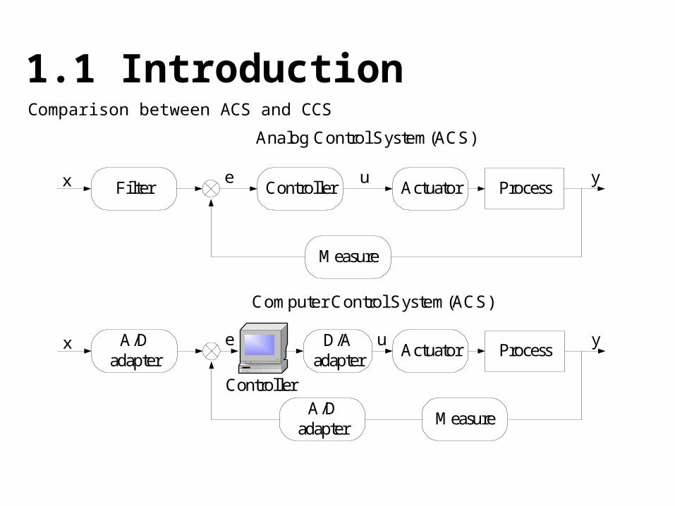
ACS CCS

Process

Actuator

Measure

Controller (correcting network)

Structure:

Process

Actuator

Measure

Controller (digital computer)

Adapter (A/D, D/A)

Parts: Analog Analog + Digital

Signals: Analog

Continuous analog

Discrete analog

Discrete digital

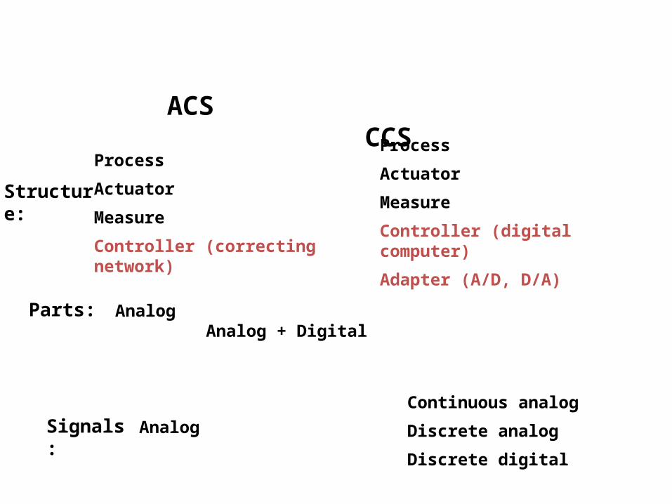
Discrete (Sampling) System1 Introduction

2 Z-transform

3 Mathematical describing of the sampling systems

4 Time-domain analysis of the sampling systems

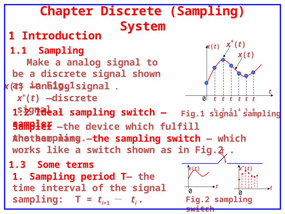
Chapter Discrete (Sampling) System

Make a analog signal to be a discrete signal shown as in Fig.1 .

t

x(t)

0 t1 t2 t3 t4 t5 t6

Fig.1 signal sampling

x(t)x*(t)

x(t) —analog signal .x*(t) —discrete signal .

1.2 Ideal sampling switch —sampler

Sampler —the device which fulfill the sampling. Another name —the sampling switch — which works like a switch shown as in Fig.2 . T

t

x*(t)

0 t

x(t)

0

Fig.2 sampling switch

1.3 Some terms1. Sampling period T— the time interval of the signal sampling: T = ti+1 － ti .

1 Introduction1.1 Sampling

1.3 Some terms2. Sampling frequency ωs — ωs = 2π fs = 2π / T .

3. Periodic Sampling — the sampling period Ts = constant.

4. Variable period sampling — the sampling period Ts≠constant.

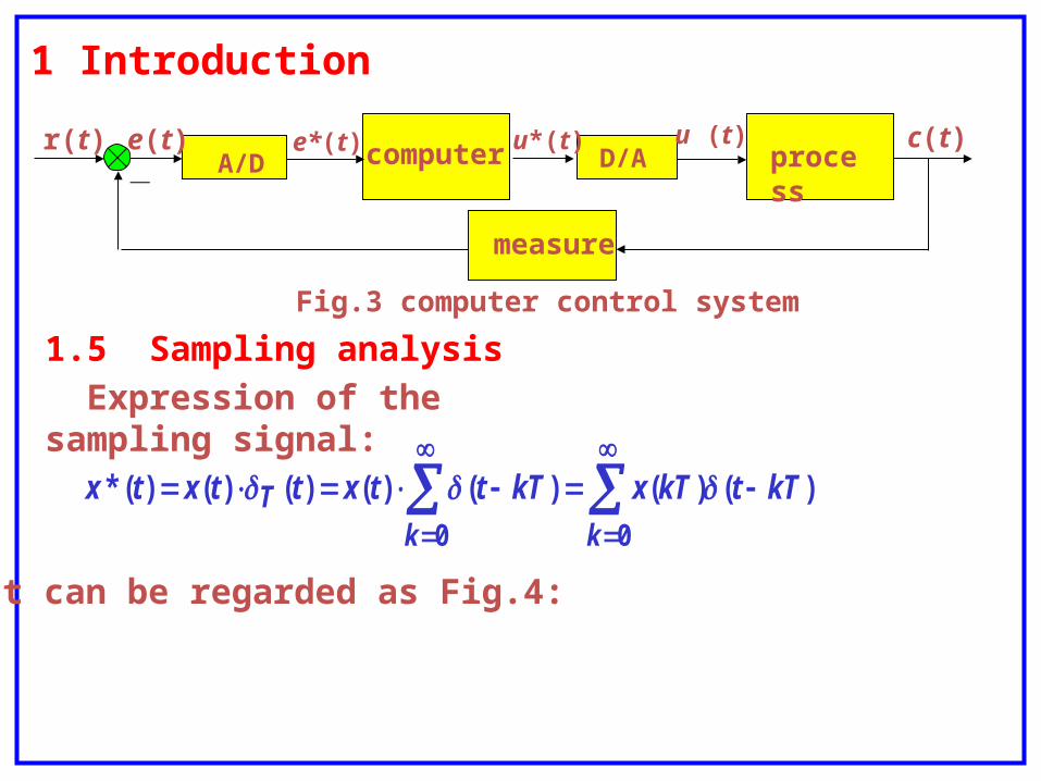
1.4 Sampling (or discrete) control system

There are one or more discrete signals in a control system —

the sampling (or discrete) control system. For example the

digital computer control system:

A/D D/Acomputer process

measure

r(t) c(t)e(t)

－e*(t) u*(t) u (t)

Fig.3 computer control system

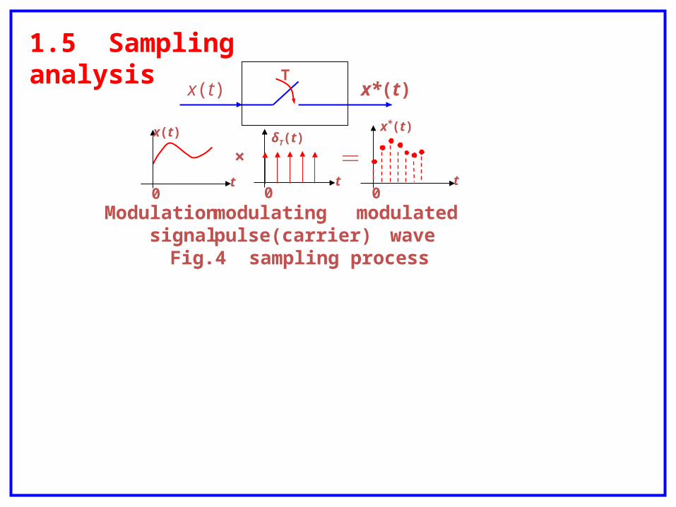
1.5 Sampling analysis

Expression of the sampling signal:

1 Introduction

)()()()()()()(*

00

kTtkTxkTttxttxtx

kkT

It can be regarded as Fig.4:

0 t

x*(t)

t

x(t)

0

T

t

δT(t)

0

× ＝

modulating pulse(carrier)

modulated wave

Modulation signal

Fig.4 sampling process

x(t) x*(t)

1.5 Sampling analysis

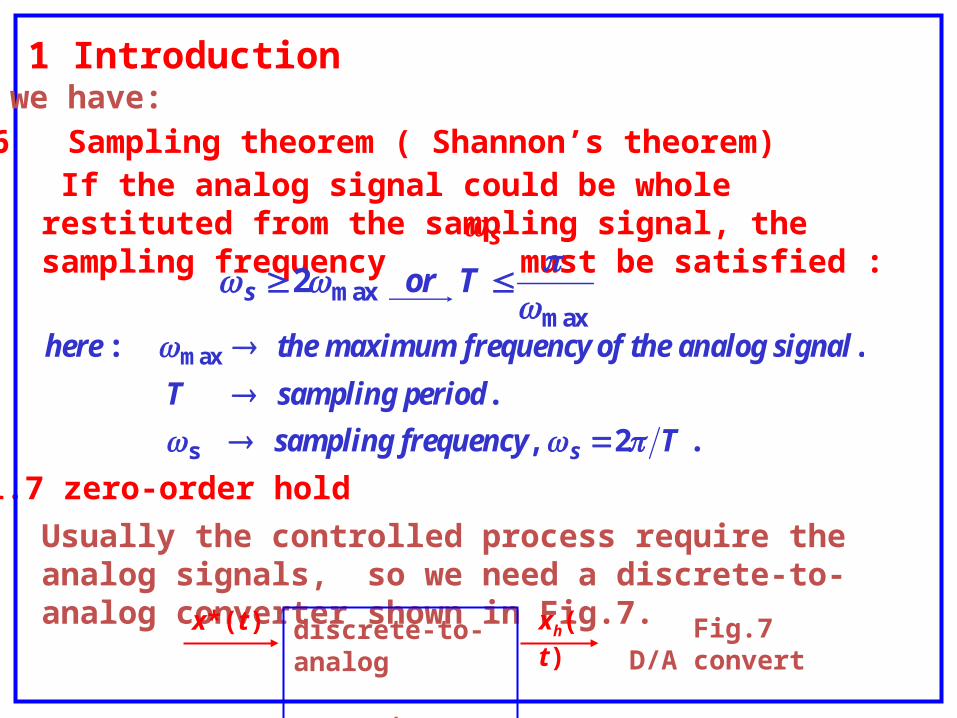
If the analog signal could be whole restituted from the sampling signal, the sampling frequency must be satisfied : s

maxmax 2

Tors

. 2 ,

.

. :

s

max

Trequencysampling f

eriodsampling pT

alnalog signy of the am frequencthe maximuhere

s

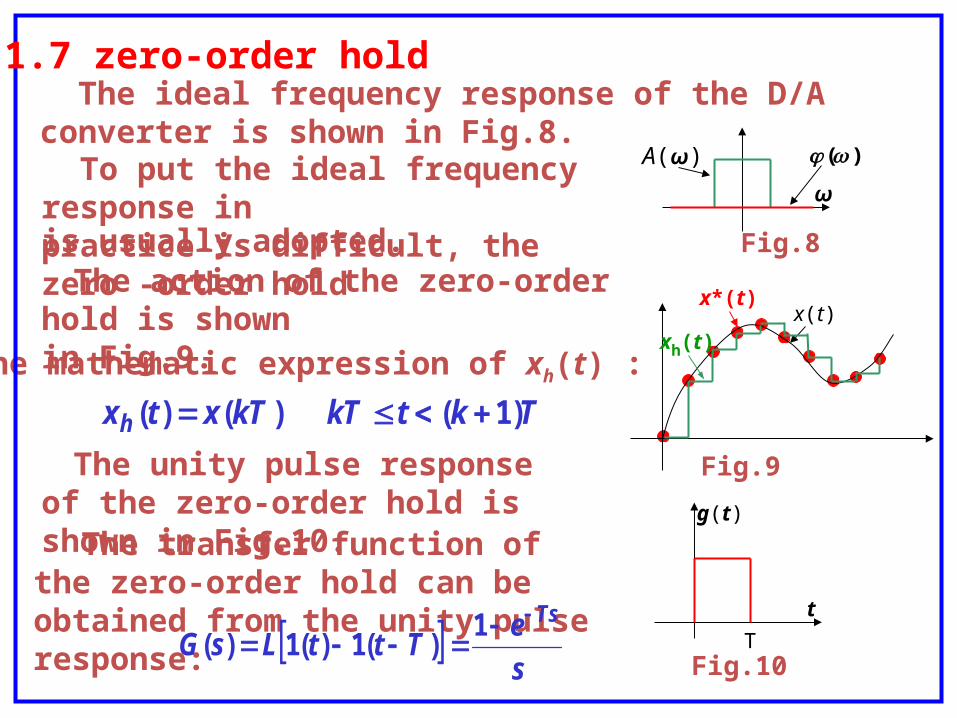
1.7 zero-order hold

Usually the controlled process require the analog signals, so we need a discrete-to-analog converter shown in Fig.7.

discrete-to-analog converter

x*(t) xh(t) Fig.7D/A convert

So we have:

1.6 Sampling theorem ( Shannon’s theorem)

1 Introduction

x*(t)x(t)

xh(t)

Fig.9

The action of the zero-order hold is shown in Fig.9.

The unity pulse response of the zero-order hold is shown in Fig.10.

The mathematic expression of xh(t) :

TktkTkTxtxh )1( )()(

The transfer function of the zero-order hold can be obtained from the unity pulse response:

s

eTttLsG

Ts

1)(1)(1)( T

Fig.10

t

g(t)

ω

A(ω) )(

Fig.8

To put the ideal frequency response inpractice is difficult, the zero -order hold is usually adopted.

1.7 zero-order hold The ideal frequency response of the D/A converter is shown in Fig.8.

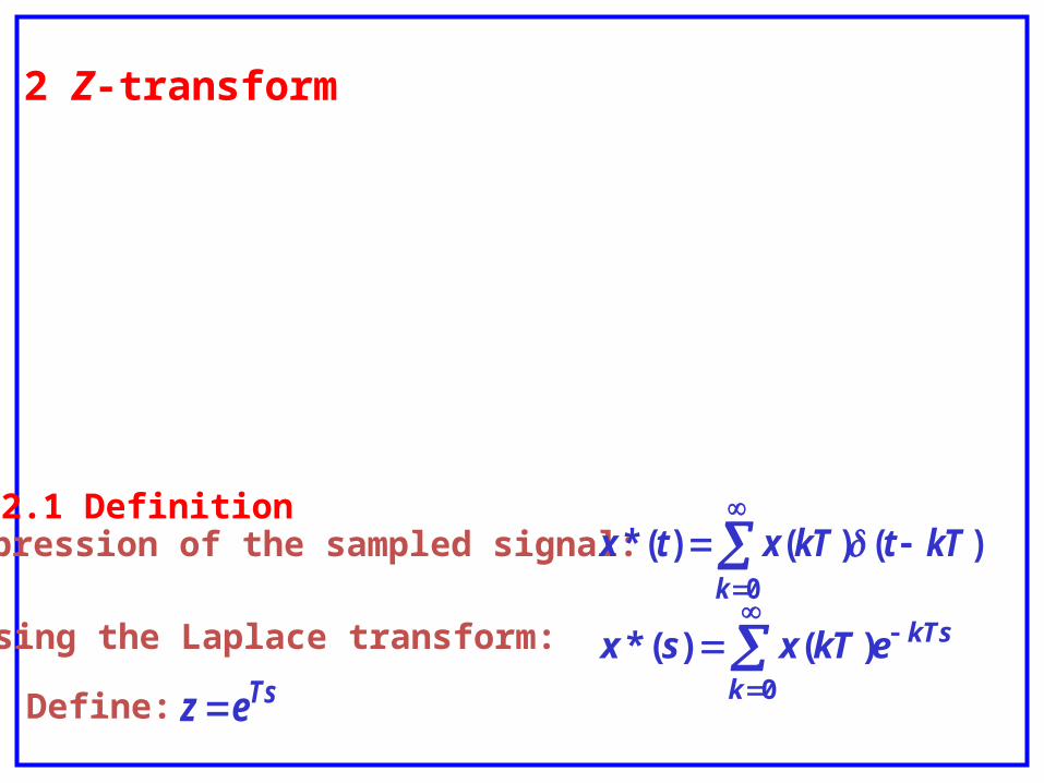
2 Z-transform

2.1 DefinitionExpression of the sampled signal: )()()(*

0

kTtkTxtxk

Using the Laplace transform:

0

)()(*k

kTsekTxsx

Define: Tsez

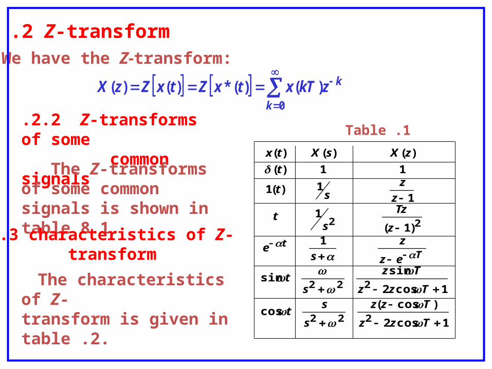
We have the Z-transform:

0

)()(*)()(k

kzkTxtxZtxZzX

.2.2 Z-transforms of some common signals

The Z-transforms of some common signals is shown in table 8.1.

.2 Z-transform

1cos2

)cos(cos

1cos2

sinsin

1)1(

1

11)(1

11)(

)()()(

222

222

22

Tzz

Tzz

s

st

Tzz

Tz

st

ez

z

se

z

Tz

st

z

zst

t

zXsXtx

Tt

Table .1

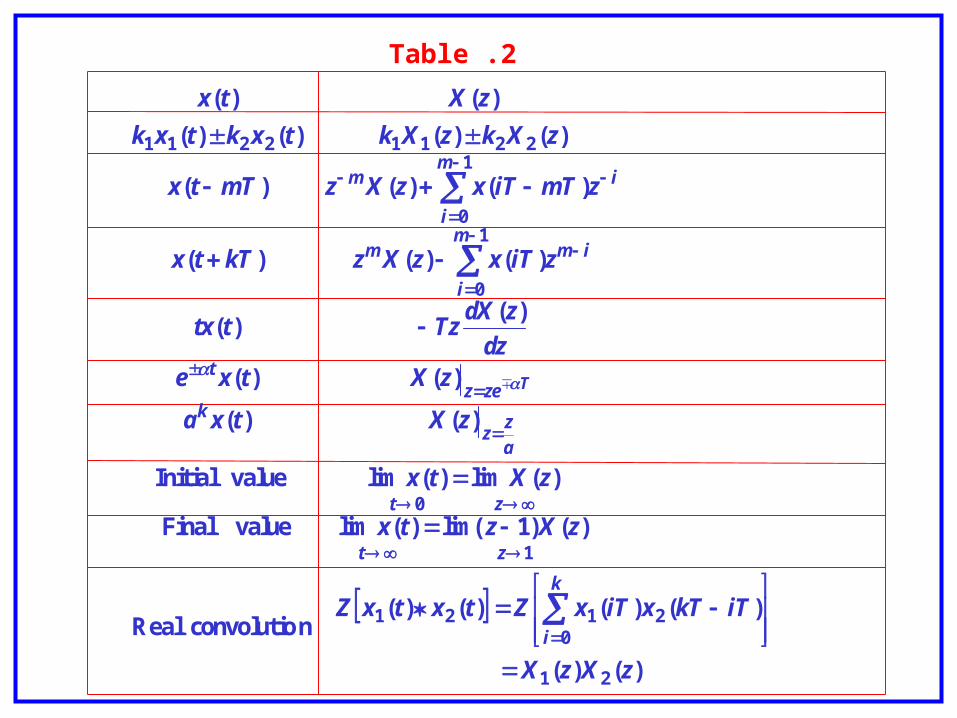
.2.3 characteristics of Z- transform

The characteristics of Z-transform is given in table .2.

)()(

)()()()(nconvolutio Real

)()1lim()(lim value Final

)(lim)(lim value Initial

)()(

)()(

)()(

)()()(

)()()(

)()()()(

)()(

21

02121

1

0

1

0

1

0

22112211

zXzX

iTkTxiTxZtxtxZ

zXztx

zXtx

zXtxa

zXtxedz

zdXTzttx

ziTxzXzkTtx

zmTiTxzXzmTtx

zXkzXktxktxk

zXtx

k

i

zt

zt

a

zz

kzez

t

m

i

imm

m

i

im

T

Table .2

m

a

zz

k

T

T

zez

t

T

T

T

zmkt

z

zzT

z

Tz

dz

dTzt

az

z

z

za

ez

Tze

z

Tzte

ezz

ze

ez

z

z

ze

zXtx

T

t

)(

)1(

)1(

)1(

1

)()1(

))(1(

)1(

11

)()(

3

2

22

22

Table .3

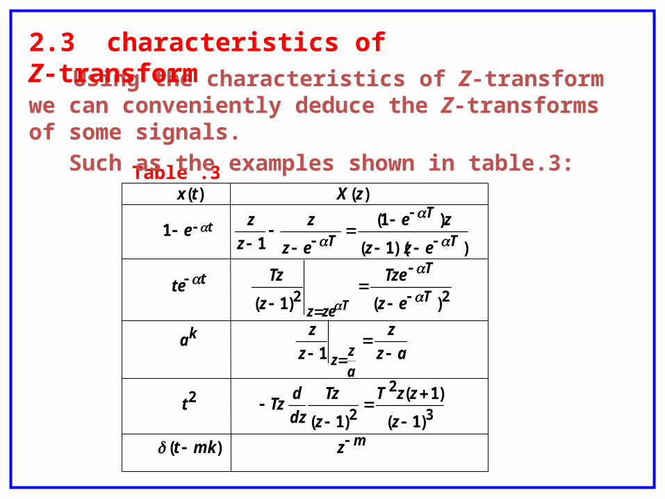
Using the characteristics of Z-transform we can conveniently deduce the Z-transforms of some signals.

Such as the examples shown in table.3:

2.3 characteristics of Z-transform

n

iTa

i

n

n

n

iez

zKzXthen

as

K

as

K

as

K

asasas

A(s)X(s)If

1

2

2

1

1

21

)( :

)())(( :

Example .1

TT ez

z

ez

z

z

z

sssZ

sss

sZ

2

515

1

10

2

5

1

1510

)2)(1(

)4(5

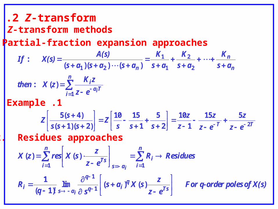
2. Residues approaches

of X(s)r polesFor q-ordeez

zsXas

sqR

ResiduesRez

zsXreszX

Tsq

iq

q

asi

n

ii

as

n

iTs

i

i

)()(

lim)1(

1

)()(

1

1

11

！

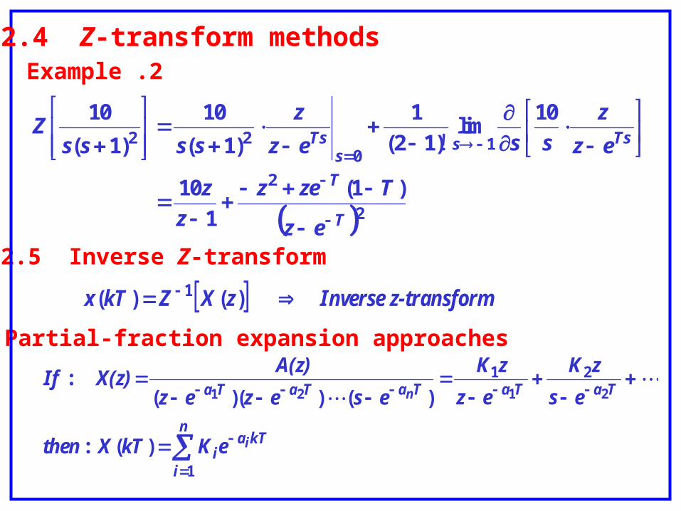
.2 Z-transform2.4 Z-transform methods

1. Partial-fraction expansion approaches

22

10

22

)1(

1

10

10lim

)12(

1

)1(

10

)1(

10

T

T

Tsss

Ts

ez

Tzez

z

z

ez

z

ssez

z

ssssZ

！

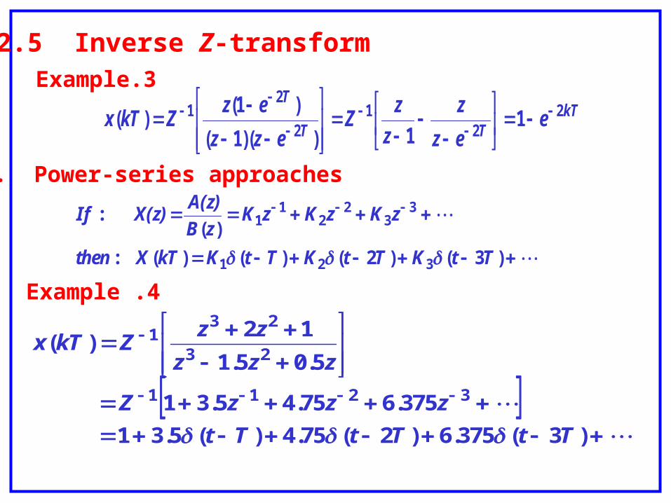
2.5 Inverse Z-transform

transformInverse z-zXZkTx )()( 1

1. Partial-fraction expansion approaches

n

i

kTai

TaTaTaTaTa

i

n

eKkTXthen

es

zK

ez

zK

esezez

A(z)X(z)If

1

21

)( :

)())(( :

2121

Example .2

2.4 Z-transform methods

kTTT

T

eez

z

z

zZ

ezz

ezZkTx 2

21

2

21 1

1))(1(

)1()(

2. Power-series approaches

)3()2()()( :

)( :

321

33

22

11

TtKTtKTtKkTXthen

zKzKzKzB

A(z)X(z)If

Example .4

)3(375.6)2(75.4)(5.31

375.675.45.31

5.05.1

12)(

3211

23

231

TtTtTt

zzzZ

zzz

zzZkTx

Example.3

2.5 Inverse Z-transform

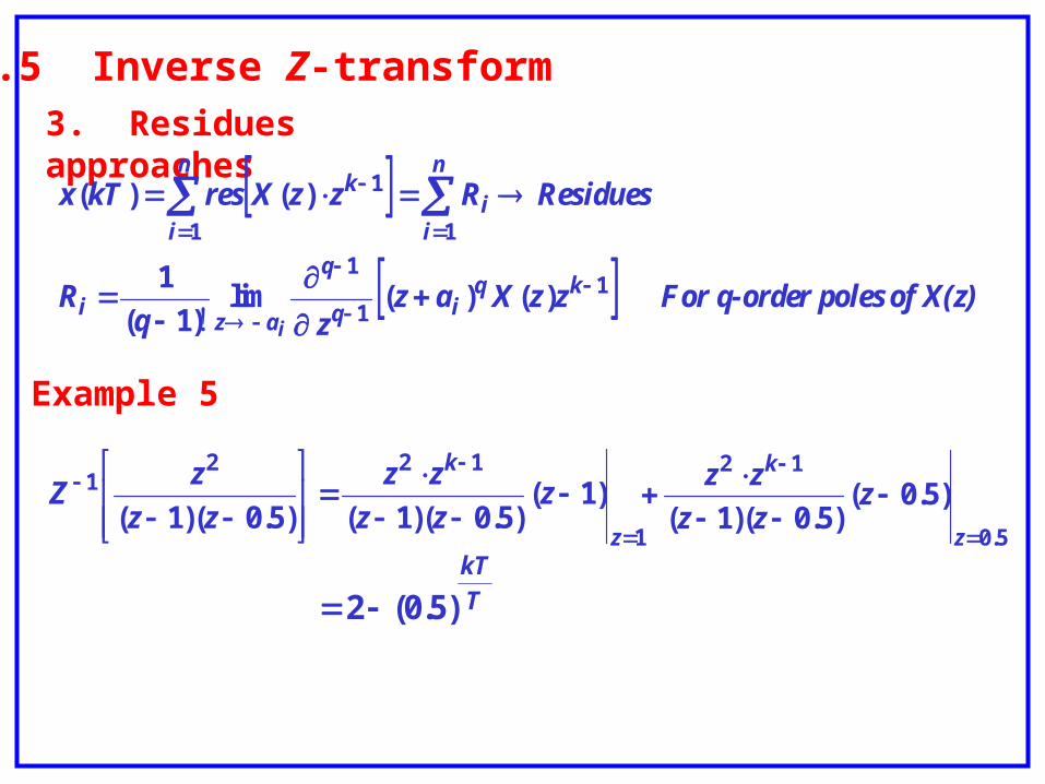
3. Residues approaches

of X(z)r polesFor q-ordezzXazzq

R

ResiduesRzzXreskTx

kqiq

q

azi

n

ii

n

i

k

i

)()(

lim)1(

1

)()(

11

1

11

1

！

2.5 Inverse Z-transform

Example 5

1

1221 )1(

)5.0)(1()5.0)(1(

z

k

zzz

zz

zz

zZ

5.0

12

)5.0()5.0)(1(

z

k

zzz

zz

T

kT

)5.0(2

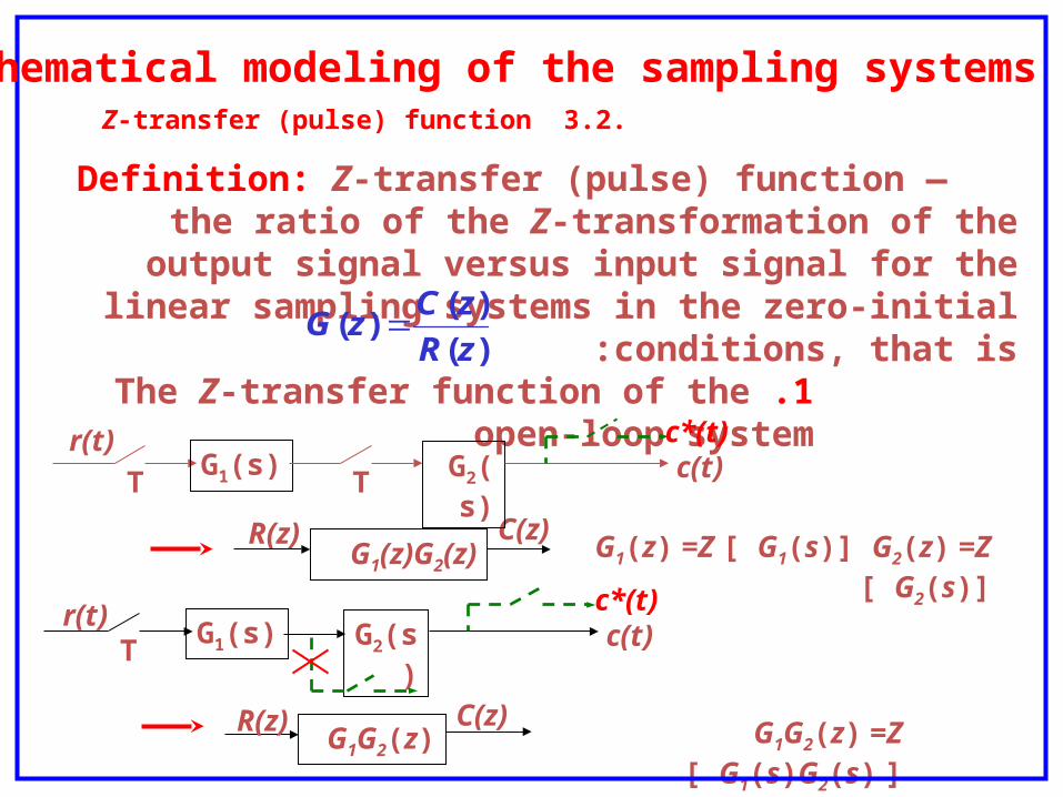
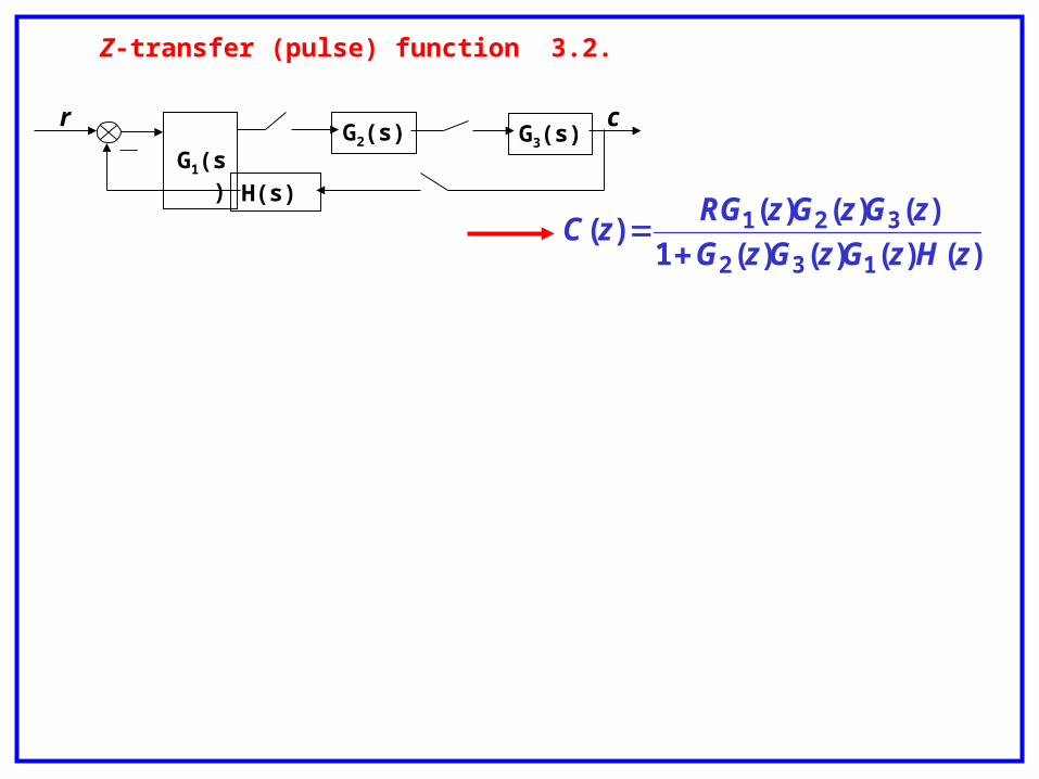
.3.2 Z-transfer (pulse) function

Definition: Z-transfer (pulse) function — the ratio of the Z-transformation of the output signal versus input signal for the

linear sampling systems in the zero-initial conditions, that is:

)(

)()(

zR

zCzG

1. The Z-transfer function of the open-loop system

TG1(s)

r(t)G2(s) c(t)

c*(t)

G1(z)G2(z)R(z) C(z)

G1(s) G2(s)

T T

r(t)c(t)

c*(t)

G1G2(z)R(z) C(z)

G1G2(z) =Z [ G1(s)G2(s) ]

.3 Mathematical modeling of the sampling systems

G1(z) =Z [ G1(s)] G2(z) =Z [ G2(s)]

G(s)r c

－H(s)

rG2(s)

c－

G1(s)

H(s)

r－

G2(s)c

G1(s)

H(s)

r c－

G(s)

H(s)

r－

cG(s)

H(s)

)()()( )(

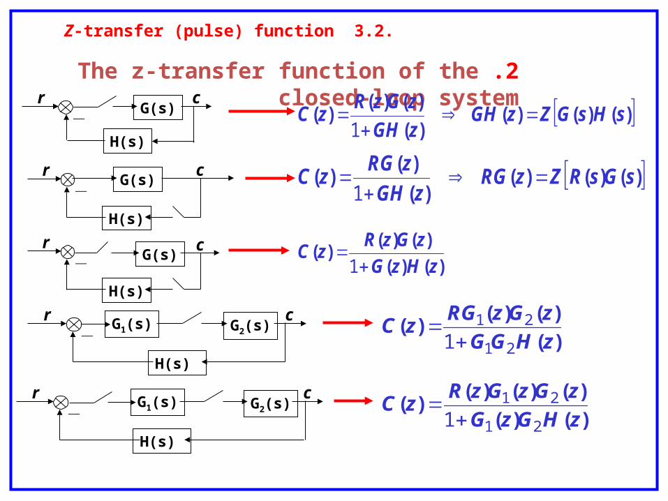
)()()( sHsGZzGH

zGH

zGzRzC

1

)()()( )(

)()( sGsRZzRG

zGH

zRGzC

1

)()(

)()()(

zHzG

zGzRzC

1

)(

)()()(

zHGG

zGzRGzC

21

21

1

)()(

)()()()(

zHGzG

zGzGzRzC

21

21

1

.3.2 Z-transfer (pulse) function

2. The z-transfer function of the closed-loop system

r－

G3(s)c

G2(s)

H(s)

G1(s)

)()()()(1

)()()()(

132

321

zHzGzGzG

zGzGzRGzC

.3.2 Z-transfer (pulse) function

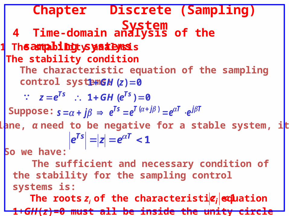
Chapter Discrete (Sampling) System4 Time-domain analysis of the sampling systems4.1 The stability analysis

The characteristic equation of the sampling control systems:0)(1 zGH

0)(1 TsTs eGHez∵Suppose: TjTjTTs eeeejs )(

In s-plane, α need to be negative for a stable system, it means:

1 TTs eze

So we have:

The sufficient and necessary condition of the stability for the sampling control systems is: The roots zi of the characteristic equation 1+GH(z)=0 must all be inside the unity circle of the z-plane, that is: 1iz

1. The stability condition

1

Re

Imz-plane

Stable zone

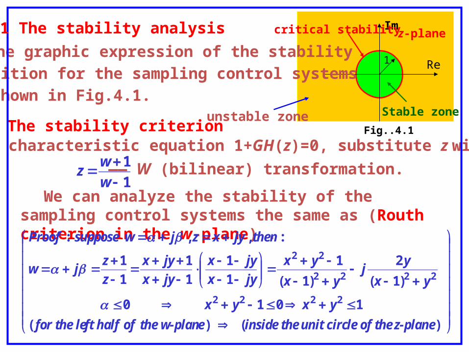
Fig..4.1

The graphic expression of the stability

condition for the sampling control systems

is shown in Fig.4.1.

2. The stability criterionIn the characteristic equation 1+GH(z)=0, substitute z with

1

1

w

wz —— W (bilinear) transformation.

We can analyze the stability of the sampling control systems the same as (Routh criterion in the w-plane) .

)( ) (

101 0

)1(

2

)1(

1

1

1

1

1

1

1

: , , :

2222

2222

22

z-planele of the unit circinside theethe w-planofft halffor the le

yxyx

yx

yj

yx

yx

jyx

jyx

jyx

jyx

z

zjw

thenjyxzjwsupposeProof

4.1 The stability analysis

unstable zone

critical stability

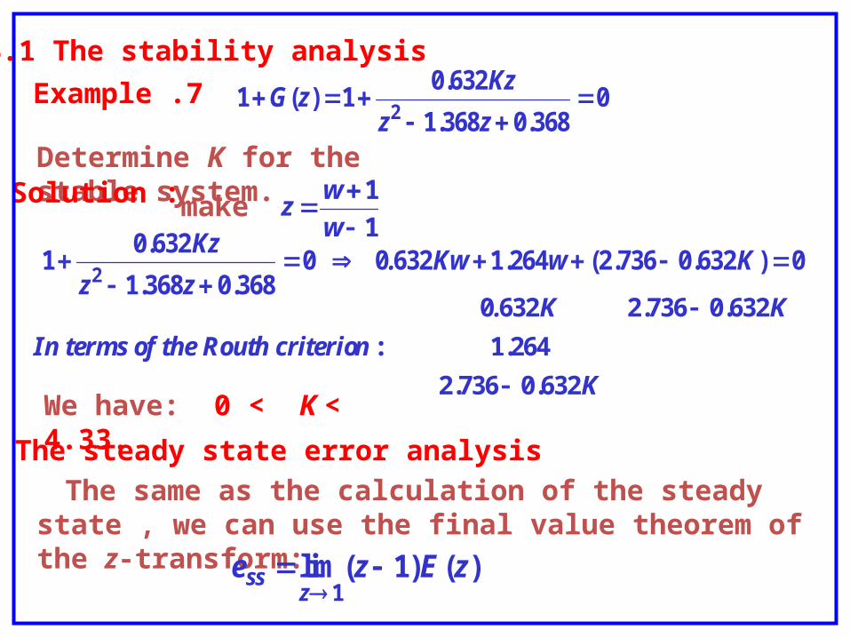
0368.0368.1

632.01)(1

2

zz

KzzG

Determine K for the stable system.Solution :

0)632.0736.2(264.16320 0368.0368.1

632.01

2

KwKw.

zz

Kz

K

KK.

nh criteriof the RoutIn terms o

632.0736.2

264.1

632.0736.26320

:

We have: 0 < K < 4.33.

1

1

w

wzmake

4.2 The steady state error analysis

The same as the calculation of the steady state , we can use the final value theorem of the z-transform:

)()1(lim1

zEzez

ss

4.1 The stability analysis

Example .7

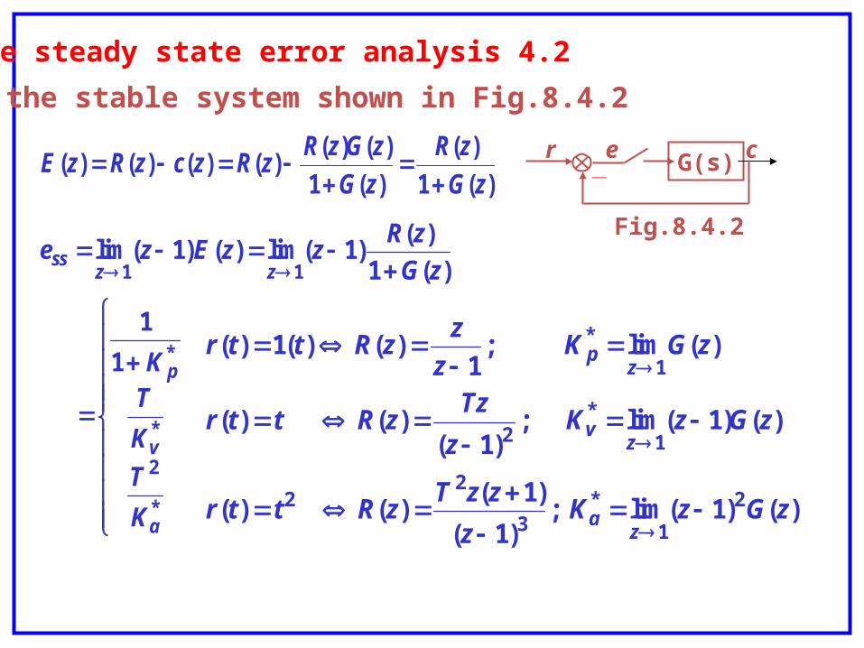
4.2 The steady state error analysis

)(1

)(

)(1

)()()()()()(

zG

zR

zG

zGzRzRzczRzE

G(s)r c

－e

Fig.8.4.2

For the stable system shown in Fig.8.4.2

*

2

*

*

11

1

1

)(1

)()1(lim)()1(lim

a

v

p

zzss

K

T

K

TK

zG

zRzzEze

)()1(lim ;)1(

)1()( )(

)()1(lim ;)1(

)( )(

)(lim ;1

)()(1)(

2

1

*3

22

1

*2

1

*

zGzKz

zzTzRttr

zGzKz

TzzRttr

zGKz

zzRttr

za

zv

zp

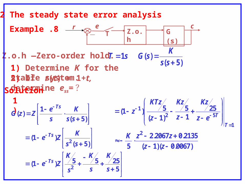
Z.o.h —Zero-order hold.)5(

)( 1

ss

KsGsT

2) If r(t) = 1+t, determine ess= ？1) Determine K for the stable system.

Solution

Example .8

4.2 The steady state error analysis

52555)1(

)5()1(

)5(

1)(

2

2

s

K

s

K

s

KZe

ss

KZe

ss

K

s

eZzG

Ts

Ts

Ts1)

)0067.0)(1(

2135.02067.2

5

2515

)1(5)1(

2

1

521

zz

zzK

ez

Kz

z

Kz

z

KTzz

T

T

r－ G (s)

cZ.o.hT

e

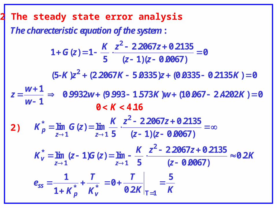
0)4202.2067.10()1.5739.993(0.9932 1

1

0)2135.00335.0()0335.52067.2()5(

0)0067.0)(1(

2135.02067.2

51)(1

:

2

2

KwKww

wz

KzKz-K

zz

zzKzG

m the systequation ofteristic eThe charec

4.2 The steady state error analysis

16.40 K

2)

KK

T

K

T

Ke

Kz

zzKzGzK

zz

zzKzGK

vpss

zzv

zzp

5

2.00

1

1

2.0)0067.0(

2135.02067.2

5lim)()1(lim

)0067.0)(1(

2135.02067.2

5lim)(lim

1T**

2

11

*

2

11

*

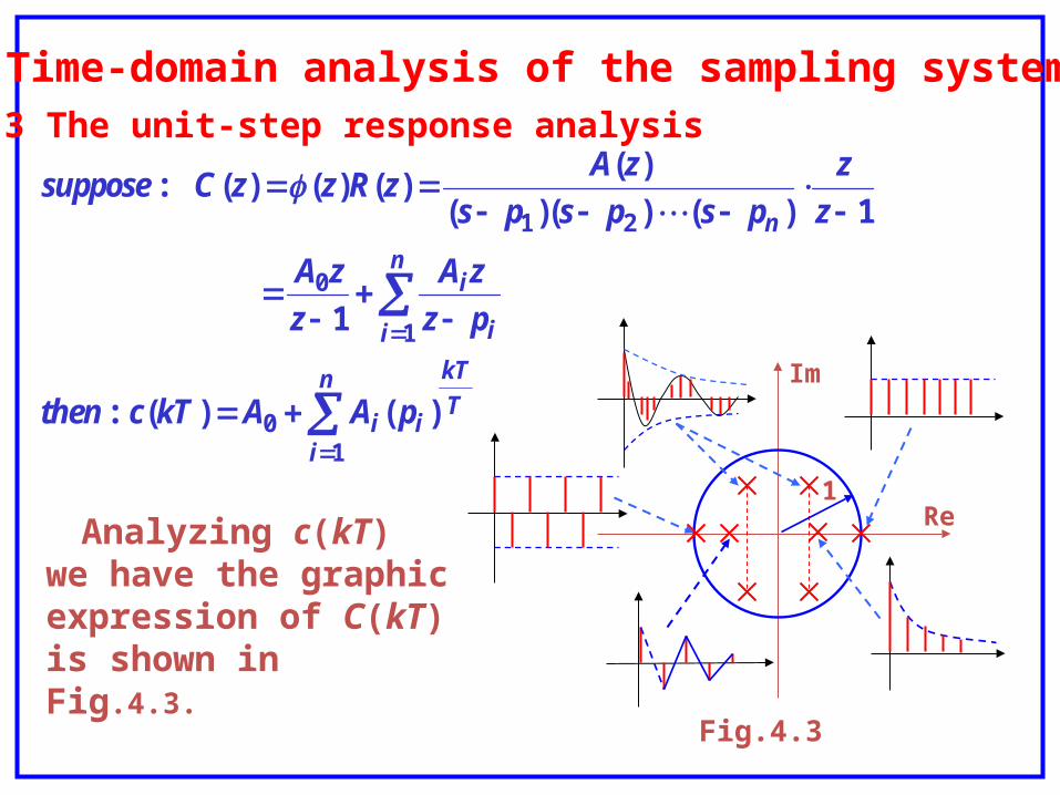
4 Time-domain analysis of the sampling systems4.3 The unit-step response analysis

n

i

T

kT

ii

n

i i

i

n

pAAkTcthen

pz

zA

z

zA

z

z

pspsps

zAzRzzCsuppose

10

1

0

21

)()( :

1

1)())((

)()()()( :

Fig.4.3

Analyzing c(kT) we have the graphic expression of C(kT) is shown in Fig.4.3.

Im

Re1

Chapter Discrete (Sampling) System

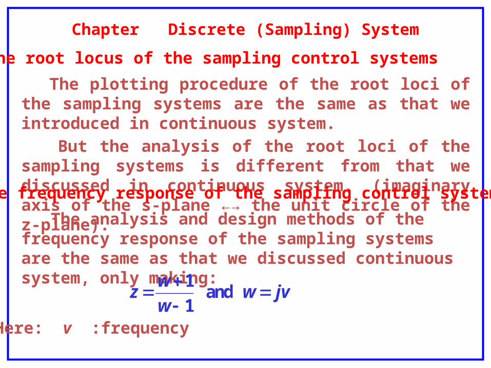
5 The root locus of the sampling control systems

The plotting procedure of the root loci of the sampling systems are the same as that we introduced in continuous system.

But the analysis of the root loci of the sampling systems is different from that we discussed in continuous system. (imaginary axis of the s-plane ←→ the unit circle of the z-plane)..6 The frequency response of the sampling control systems

The analysis and design methods of the frequency response of the sampling systems are the same as that we discussed continuous system, only making:

jvww

wz

and 1

1

Here: v :frequency

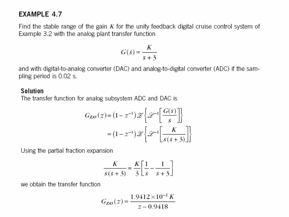
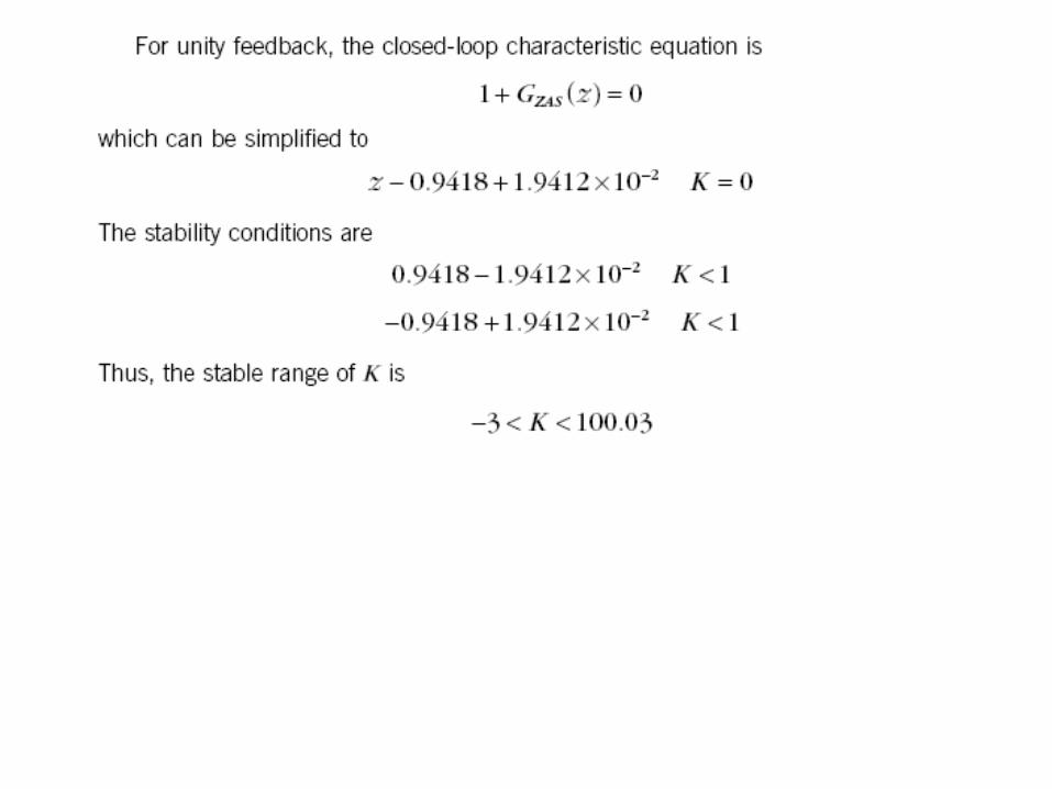
Stability of Digital Control System

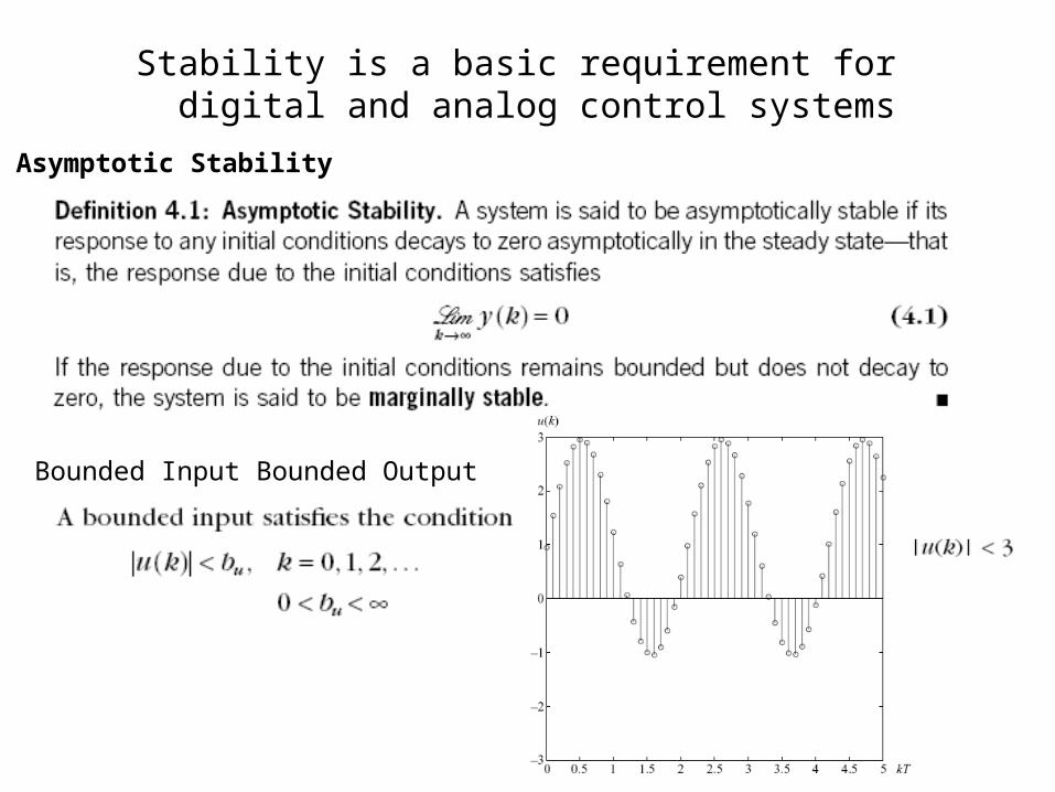
Stability is a basic requirement for digital and analog control systems

Asymptotic Stability

Bounded Input Bounded Output

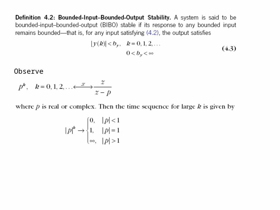
Observe

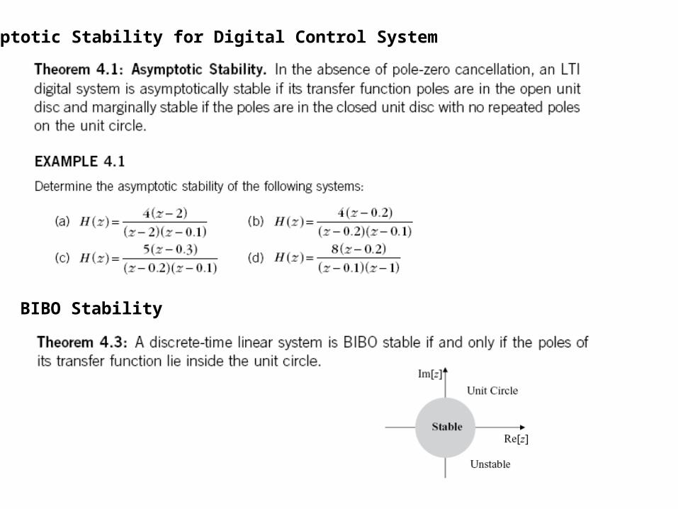
Asymptotic Stability for Digital Control System

BIBO Stability

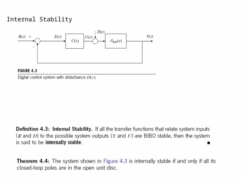
Internal Stability

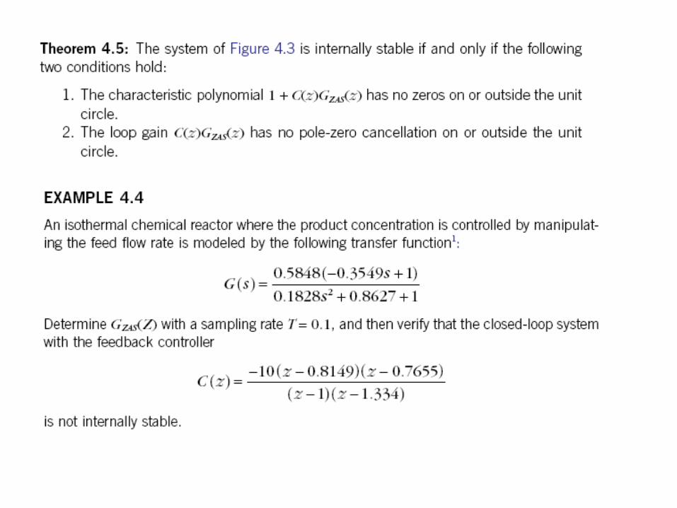
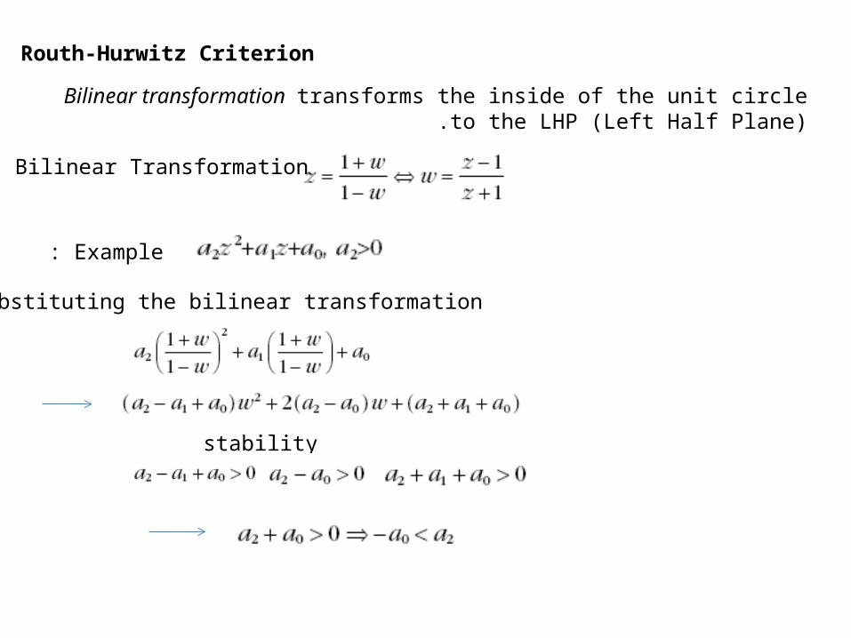
Routh-Hurwitz Criterion

Bilinear transformation transforms the inside of the unit circle to the LHP (Left Half Plane).

Bilinear Transformation

Example:

Substituting the bilinear transformation

stability conditions

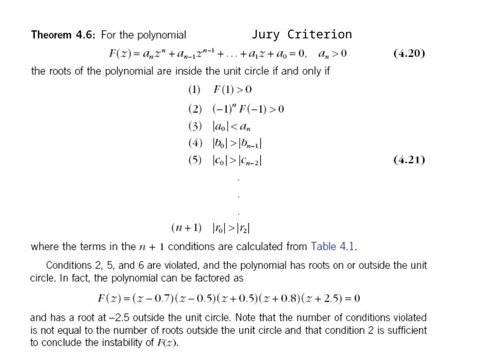
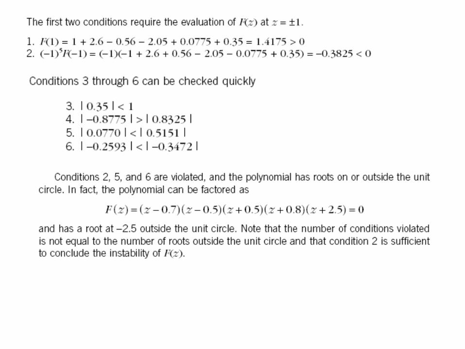
Jury Criterion

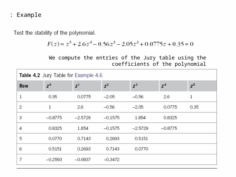
Example:

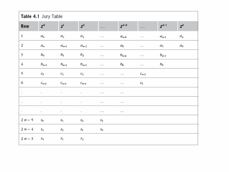
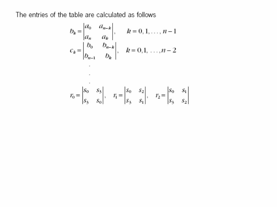
We compute the entries of the Jury table using the coefficients of the polynomial

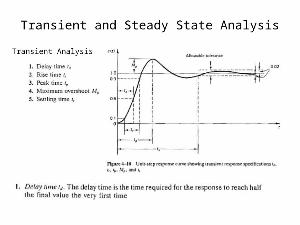
Transient and Steady State Analysis

Transient Analysis

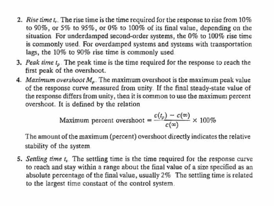
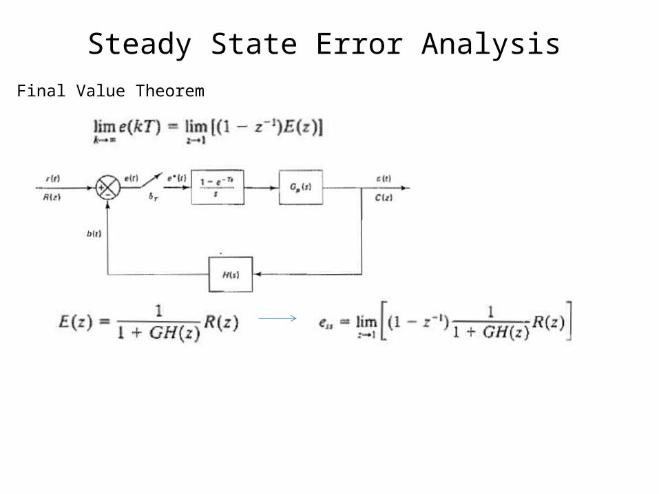
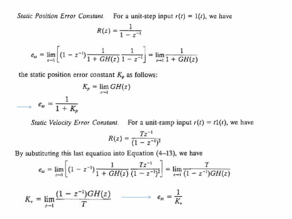
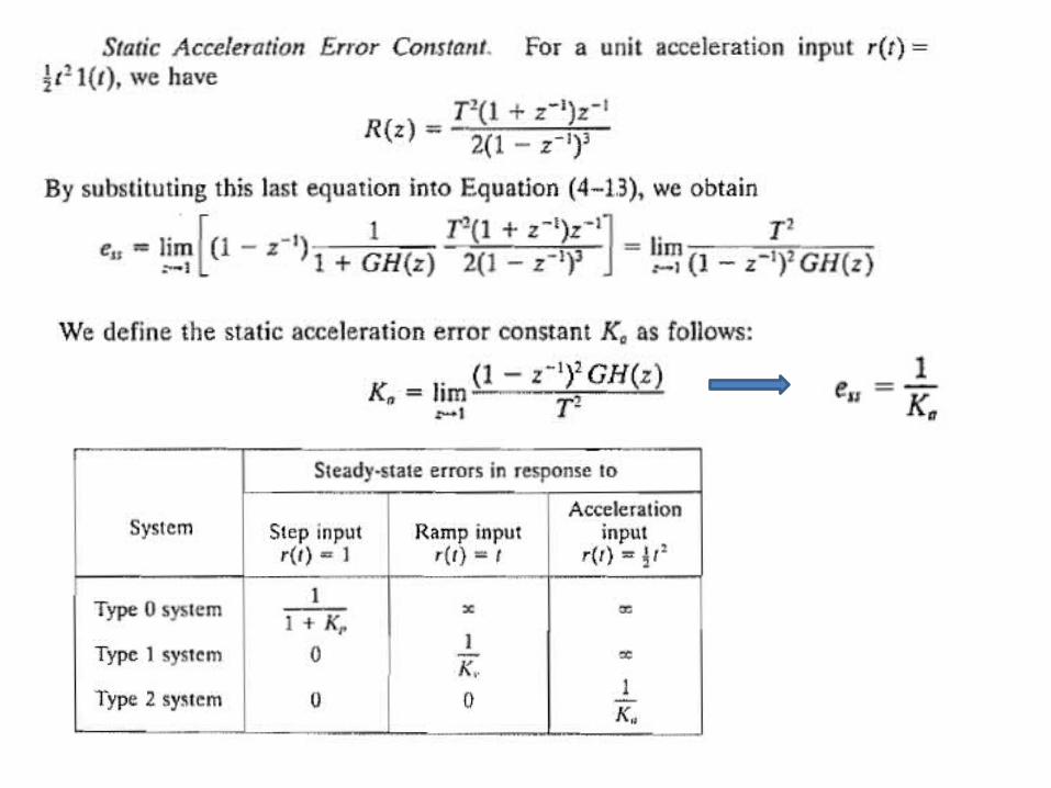
Steady State Error AnalysisFinal Value Theorem

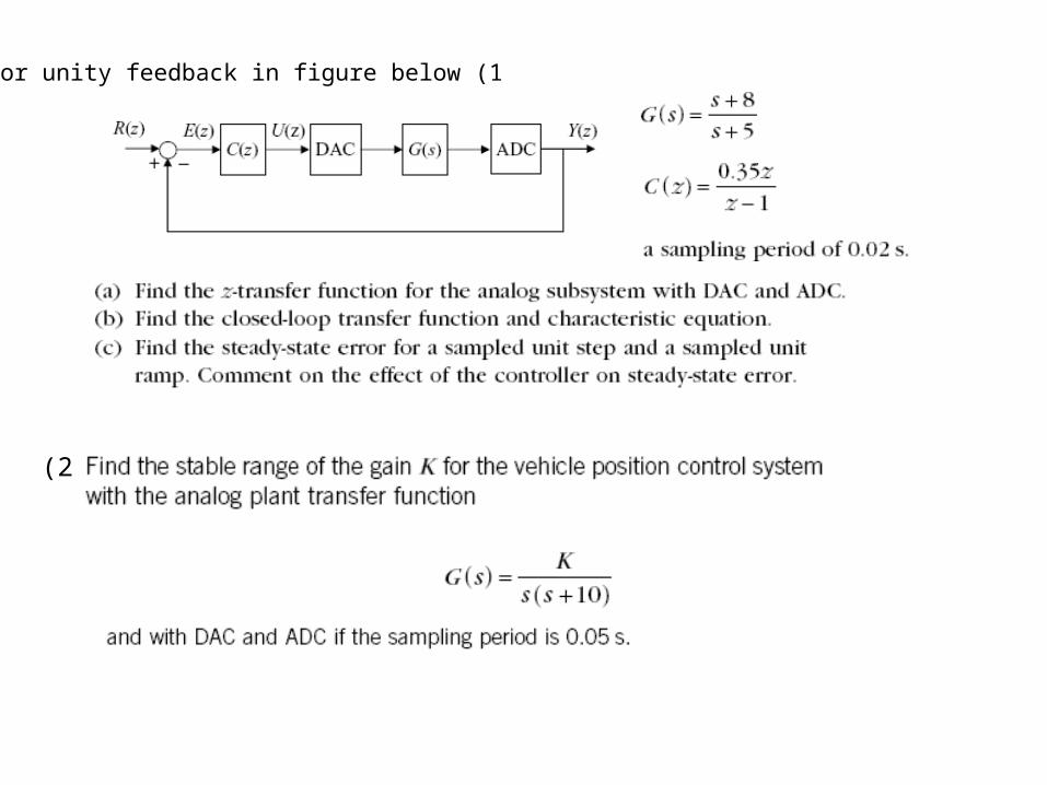
1 )For unity feedback in figure below,

2)