Embed Size (px)
Citation preview
/
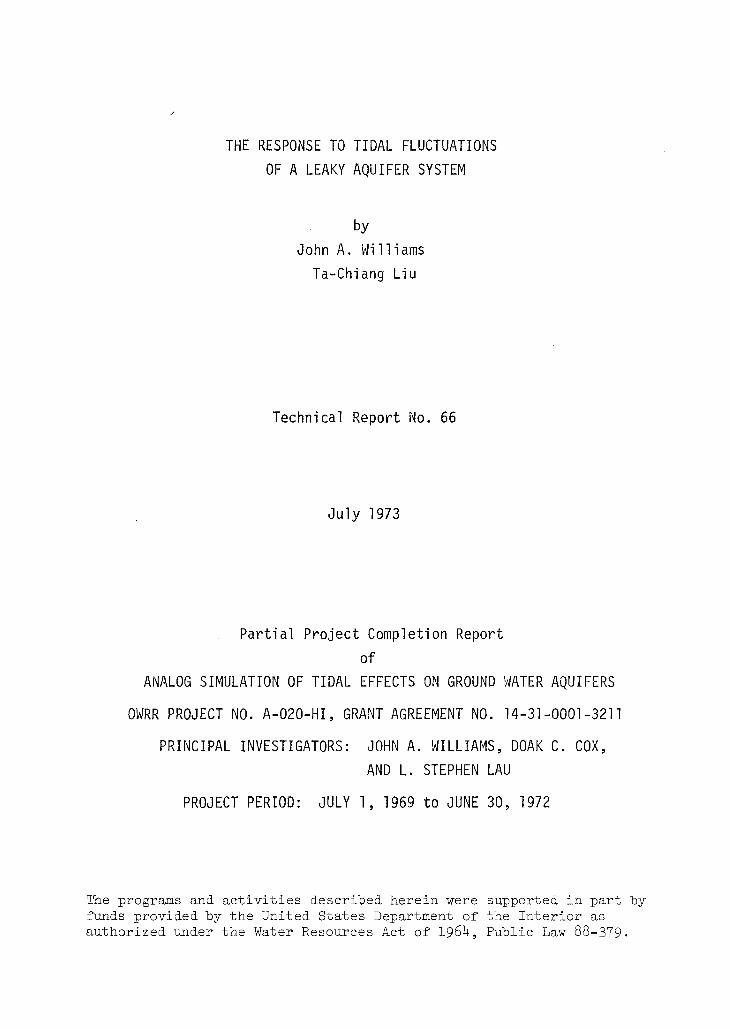
THE RESPONSE TO TIDAL FLUCTUATIONS OF A LEAKY AQUIFER SYSTEM
by
John A. \~i 11 i ams Ta-Chiang Liu
Technical Report No. 66
July 1973
Partial Project Completion Report of
ANALOG SIMULATION OF TIDAL EFFECTS ON GROUND LI/ATER AQUIFERS
OWRR PROJECT NO. A-020-HI, GRANT AGREEMENT NO. 14-31-0001-3211
PRINCIPAL INVESTIGATORS: JOHN A. WILLIAMS, DOAK C. COX, AND L. STEPHEN LAU
PROJECT PERIOD: JULY 1, 1969 to JUNE 30, 1972
The programs and activities descrioed herein were supported in part by funds provided by the United States Department of the Interior as authorized under the Water Resources Act of 1964, Public Law 88-379.

ABSTRACT
A system of two isotropic and homogeneous infinite aquifers, which are separated by an aquitard and subject to tidal fluctuations along their coastal boundary, has been analyzed and a mathematical model has been developed for the response of this system to tidal changes. The mathematical model consists of equations for the amplitude and phase of the response of both aquifers to a periodic tide. A computer program using the IBM 560 has been written for the evaluation of these equations. Both the mathematical model and the program have been verified by an electric analog model constructed for that purpose.
The mathematical model was evaluated for an aquifer system where both aquifers have the same transmissability (and therefore the same leakage factor) but where the storage of the upper aquifer was 100 times that of the lower aquifer. Tidal periods of 0.5, 1, and 14 days were used. The results indicate that deviations from a response corresponding to the no-leakage case could be from 50 to 100 percent or more for both the amplitude and the phase angle of either aquifer. Also, such deviations were produced by a relatively moderate amount of leakage, i.e., 1/B2 : 0.154 x 10-~ ft- 2.
iii
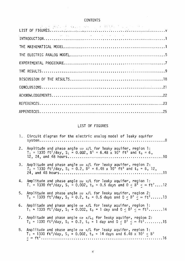
CONTENTS
LIST OF FIGURES •• "~.' ••. , ••.. ,., .... ,.;,.~ ••••.• : .• , .• , •• ; •..•• ' ••. ; .•• ~ ..•••••••.••••• V
, . INTRODUCTION ••.•••••••••••••.••••.••••.•••.•••••••••••.••••.•.••.•••.••. 1
THE MATHEMATICAL MODEL .••••.••••••.•••....•.•.••••••••.•••••.•••• ',' ••••. 1
THE ELECTRIC ANALOG MODEL ............................................... 5
EXPERIMENTAL PROCEDURE .•••..•••.••...••...•••.•..•••••••••.•••••••••••.. 7
THE RESULTS .•.•••.•.••.•••••••••••••.•..•••••••••••••..• ~ .•.•••••••.•••• 9
DISCUSSION OF THE RESULTS .............................................. 18
CONCLUS IONS ••.•••.•.•••••••..••.•.••.••••••••••••••••.••.•..•••.••.•••• 21
ACKNOWLEDGEMENTS .•••.••••••.••••.••••••.•.••..•.••...•••.•••.••.••....• 22
REFERENCES •••••.••..•....•••••••.••••••.•••••..••••.•..•.•.•••••••.•..• 23
APPENDICES •••.•••••••••••......•••.•••.••••••.•••...••.•.•••••••••.••.• 25
LIST OF FIGURES
1. Circuit diagram for the electric analog model of leaky aquifer system .............................................................. 8
2. Amplitude and phase angle VB x/L for leaky aquifer, region 1: T1 = 1330 ft 2/day, S1 = 0.002, 82 = 6.48 X 104 ft2 and to = 6, 12, 24, and ,48 hours ............................................... 10
3: Amplitude and phase angle VB x/L for leaky aquifer, region 2: T2 = 1330 ft 2/day, S2 = 0.2, 82 = 6.48 X 104 ft2 and to = 6, 12, 24, and 48 hours ................................................... 11
4. Amplitude and phase angle VB x/L for leaky aquifer, region 1: T1 = 1330 ft 2/day, S1 = 0.002, to = 0.5 days and a ~ 82 ~ 00 ft2 .... 12
5. Amplitude and phase angle VB x/L for leaky aquifer, region 2: T2 = 1330 ft 2/day, S2 = 0.2, to = 0.5 days and 0 ~ 82 ~ 00 ft2 ...... 13
6. Amplitude and phase angle VB x/L for leaky aquifer, region 1: T1 = 1330 ft 2/day, S1 = 0.002, to = 1 day and 0 ~ 82 ~ 00 ft2 ....... 14
7. Amplitude and phase angle VB x/L2 for leaky aquifer, region 2: T2 = 1330 ft 2/day, S2 ~ 0.2, to = 1 day and a : 82
: 00 ft2 ......... 15
8. Amplitude and phase angle VB x/L for leaky aquifer, region 1: T1 = 1330 ft 2/day, S1 = 0.002, to = 14 days and 6.48 x 10 3 < 82 < 00 ft2 .................................................... : ....... 1,6

9. Amplitude and phase angle VB x/L for leaky aquifer, region 2: T2 = 1330 ft 2/day, $2 = 0.2, to = 14 days and 6.48 x 10 3 < B2 < 00 ft 2
•••••••••••••••••••••••••••••••••••••••••••••••••• : ••••••••• 17
vi

INTRODUCTION
This report presents a continuation of the general study of the
response of coastal aquifers to tidal fluctuations. It deals specifically
with the response of an aquifer system consisting of two horizontal and
semi-infinite,aquifers separated by a semipermeable layer, or aquitard.
Both aquifers are of constant thickness, homogeneous and isotropic, and
only vertical movement of water through the aquitard is assumed.
Even though this model is highly idealized, it should yield reasona
ble estimates of the deviation of the amplitude and phase relations from
those of similar aquifers but without the presence of leakage. It also
offers a means of studying the response of a leaky aquifer under the varia
tion of any of the several parameters involved, i.e., storage, permeabili
ty, leakage factor, etc. The model, together with the two non-homogeneous
aquifer models developed previously (Williams and Liu, 1971), will help
provide a general insight into the interpretation and the use'of tidal
data for the determination of real aquifer properties which is the
ultimate goal of this research.
The Mathematical Model
The two model aquifers will be considered as one-dimensional, homo
geneous, and isotropic and their respective constants and variables dis
tinguished between by the use of subscripts: one (1) for the lower aqui
fer which is necessarily semi-confined and two (2) for the upper aquifer
which may be either confined from above or phreatic. The coastline is
located at distance L to the right of the origin of coordinates which is
in the interior of the aquifer system. A glossary of the terms used and
a sketch defining the aquifer system are presented in Appendix A.
A combination of the conservation of mass principle and Darcy's Law
together with the assumptions of Dupuit for the two aquifers and of strict
~y vertical flow in the aquitard leads to the following coupled differen
tial equations
+ = (la)

2
and
+ = (lb)
where a. = (S/T). (or E'/Kz for a phreatic aquifer) is the ratio of storage J J
to transmissability, B2. = K.b.b'/K' is the leakage factor, h. = h. (x,t) J J J J J
is the piezometric head, and x and tare the independent space and time
variables.
Since tidal fluctuations are periodic both hI and h2 may be written
as the real part of
h . (x, t) = R (I";. (x) e i crt) , J J
(2)
where cr is 2n divided by the tidal period and 1";. (x) is the space dependent J
amplitude of the fluctuation in h.(x,t). J
Elimination of t in equations (la) and (lb) by use of equation (2)
yields the following pair of ordinary differential equations, S2
Bl 2 (3a)
and
S2" - P21";2 = SI
B2 2 (3b)
where
P. 1 icra. = + J B. z J
J (4)
Equations (3a) and (3b) may be further reduced by elimination of 1";2 to
give the following fourth order equation:
S 1 "" - (P 1 + P 2) I"; 1 " + (p 1 P 2 - I ) S 1 = 0 B12B22 (5)
Equation (5) has a fourth order characteristic equation whose roots are
( f\
cos -;- + i Si<+ )

where
and
+ iq = (cos~ +
( cos :-
8
2
- ) i sin
m4 - - (p + iq ) = + i Sin~ )
[012 + 02 2 ± 1/
P± = 1/2 20102 cos (fh-82)] 2
S± - [0 1 sin Bl ± 02 sin 82 J = tan 01 cos SI ± 02 cos 82
~1 eiBI P P v = 1 + 2
= [ (PI - +
Hence, the solution to equation (5) can be written as
(6)
(7)
(8)
(9)
For aquifers which extend infinitely far in the negative x-direction,
the constants of integration Bl and Dl must be zero. With ~1 (x) deter
mined, ~2 (x) is also determined by equation (3a).
The boundary condition at x = L requires that the fluctuation in
either aquifer coincide with the tide. Thus,
~1 (L) = + = -i~o (lOa)
and
(lOb)
where ~ is the amplitude of the tide at the coastline. The equations o (lOa) and (lOb) may be solved for the remaining two constants of integra-
tion, i.e.,
Al = AIr + iA,li =
=
-i i; 0
----2 2 ml -m3
-i~o ---
3
(lla)

4
and i/;;o (llb)
Thus, for the aquifer of region 1, the amplitude function becomes
(12)
Finally, substituting equation (12) into equation (2) the expression
for the piezometric head in the lower aquifer becomes
where
and
with
hI (X,t)
PI (x) =
= tan- l
= /;;0 PI (x) sin (crt + e ) , PI
+
+
[ R 1 (L) II (x)
Rl(L)Rl(X)
Rl(X) = (AIr cos q+(x-L) - Ali sin q+(X-L)) eP+(x-L)
+ (Clr cos q_(x-L) - Cli sin q_(x_L))eP-(X-L)
Il(X) = (AIr sin q+(x-L) + Ali cos q+(X-L)) eP+(x-L)
+ (Clr sin q_(x-L) + Cli cos q_(x-L)) eP_(x-L)
(13a)
(l3b)
(l3c)
(13d)
(l3e)
The amplitude function for piezometric head in the upper aquifer, or
region 2, follows from equation (3a), i.e.,
which becomes
-i/;;o B12 [A 2eml (x-L) c2em3 (x-L)] /;;2 (x) = (14)
m12-m3 2
where
A2 = A2r + i A2i = (Pl-m1 2) Al
C2 = C2r + i C2i = (Pl-m3 2) Cl

5
on application of equations (lla) and (lIb). Substitution of equation
(14) into equation (3a) and the substitution of that result into equation
(2) gives the final expression:
where*
and
with
hdx, t) =
P2(X) =
l;;oP2(x) sin
[
R2 2 (x) l;;oB12
R12 (L)
(crt + e ) P2
= (A2r cos q (x-L) - A2i sin q (x-L)) eP+(X-L) + +
+ (C2r cos q_(x-L) - C2i sin q_(x-L)) eP_(x-L)
12(x) = (A2r sin q+(X~L) + A2i cos q+(x-L)) ep+(x-L)
+ (C2r sin q (x-L) + C2i cos q (x-L)) eP_(x-L)
(lSa)
(lSb)
(lSc)
(lSd)
(lSe)
Two special cases of the above equations, :.e., when the aquitard
becomes an aquiclude and when both aquifers are identical, are considered
in Appendix B.
THE ELECTRIC ANALOG Mon~L
The analogous electrical circuit for the leaky aquifer consists of a
parallel plate capacitor where-one of the plates acts as a conductor and a
current is permitted to "leak" into this conducting plate from some
external energy source. The differential equation representing this
situation has been derived by Knrplus (1958) and is
a2v R av + - !::,.V = RC-
(16)

6
where V is the voltage, R is the resistance per unit of length of the
capacitor plate, R.R, is the resistance of the media through which the
leakage current passes per unit of length along the capacitor plate and
6V is the voltage with respect to the conducting capacitor plate which
drives the leakage current.
Equation (la) or (lb) can be transformed into an equation similar to
(16) using the scale factors defined by Walton and Prickett (1963), i.e.,
q eft3) = K12 (coulombs)
heft) = K2V (volts)
Q(ft 3 /sec) = K3 i (amperes)
t (sec) = K4t (sec) (17) e
where the similarity between Darcy's Law and Ohmls Law and between q = Qt
and 2 = it requires that e (l8a)
and
(18b)
respectively. If the unit of length in the aquifer is "a" feet, then by
using equation (17), equation (la) or (lb) can be written as
+ (Vo-V) = at
e
A comparison of this transformed equation with equation (16) defines two
more compatibility relations:·
a 2a
RC (18c)
and R a 2 = B1 2 -
R 1
or RT RT a = b l = --.b l = b l
R (aK I) (RT) (l8d) 1 1
Equation (18d) follows from the fact that the product RT = KdK2 should
remain the same throughout,the aquifer system. Hence, in a leaky aquifer

the characteristic length "a" is no longer arbitrary but equal to the
thickness of the aquitard. The three remaining compatibility equations
are unchanged.
To apply these relations, the aquifer system is first defined; then
b' is known and "a" is fixed. Rand C can be selected for convenience
for the lower (or the upper) aquifer and K~ determined. With Kz as an
arbitrary factor, K3 and Kl can then be found by application of equations
(18b) and (18a), respectively. Values of Rand C for the upper (or the
lower) aquifer are given by the application of equations (18b) and (18c)
and Rl is determined from equation (18b).
The electric analcg model consisted of two arrays of resistors and
capacitors and corresponding nodal points in each array were connected by
a v.ariable resistor. The circuit diagram and the electrical sizes of the
components used are shown in Figure 1. Since the system involved two
aquifers of infinite extent, a sufficient number of components had to be
incorporated into the analog to produce an undetectable response at the
circuit boundary to any signal originating at the coastline. This
amounted to extending the circuit to between one and two penetration
lengths of the tide, as recommended by Williams and Liu (1971). "Lumped"
components were used to simulate the interior two-thirds of the modeled
portion of the aquifer system.
EXPERIMENTAL PROCEDURE
7
The simulated aquifer system was defined by the following values for
the pertinent parameters: L = 720 ft, Kl = 13.3 ft/day, Kz = 26.6 ft/day,
Sl = 0.002, Sz = 0.2, bl = 100 ft, bz = 50 ft, b' = 36 ft, and BIZ = Bzz = BZ = 6.48 x 10~ ft Z (i.e., K' = 0.739 ft/day). Values of 1000 ohms and 0.01
microfarads were selected for the resistance and capacitance, respectively,
for region 1. Consequently, 1000 ohms and 1.0 microfarads were the values
for the resistance and capacitance, respectively, determined for region 2.
Thus, the time scale factor K~ from equation (18b) is K~ = 195 day/sec.
Finally, it should be noted that BZ = 6.48 x 10~ ft Z corresponds to R = 1
50 R = 50,000 ohms and the variable resistors in the analog model were set
to this value.

00
NODAL POINT 0 2 3 ••• 28 29 30 40 • •• 70 80 90
Rz R z R z Rz R z 10 Rz 10 Rz 10Rz
."/1 ~/1 /1 /1 •••
= OSCILLATOR I ~ ~ ~ ~ ~ i _ 15C
Z1
C
Z1
C
ZI
C
ZI
15C
ZI
5C
ZI
10C
ZI
10C
ZI
10C
ZI
5C
Z1
- - - -- - - -
~ ~ ~ ~
RQ ~<- R~ ~> z/3 RQ
RI RI RI RI RI 10RI 10 RI 10 RI ;' 'V'V'v ) '\Nv ) 'V\/\ ;' •• • --;--....J\/I/\r---f---'WV-----7
DUAL TRACE
L5C
II
C
II
C
II
C
II
1.5C
II
5C
I1
10C
II
IOC
l1
10C
II
5C
IT
OSCILLOSCOPE
1:-'ROBE =
= = - =
®l ELECTRICAL S!ZES: NOTES: RI R z =1000.u I/Z WATT I) RA IS A POTENTIOMETER CI 0.01 p.f - 50 VDC WITH A RANGE OF 0-500 kn Cz 1.0 p.f - 50 VDC
EXT. EXCITE R~ 50,000.u - 2.5 WATTS
2) rJ = CLIP CONNECTION TO REMQ.VE Ra FROM CIRCUIT
FIGURE 1. CIRCUIT DIAGRAM FOR LEAKY AQUIFER SYSTEM.

Once the variable resistors were adjusted and the harmonic
oscillator set to give the desired frequency, the remaining step was to
place the oscilloscope probe at each of the nodal points and read and
record the amplitude and phase of the response off the oscilloscope
screen.
THE RESULTS
9
The results from both the electric analog and the mathematical model
are presented in graphs of the amplitude and the phase angle as functions
of the dimensionless position x/L. The amplitudes have been normalized
with respect to the tidal amplitude at the coast and the phase angles
represent the time required for a particular tidal phase to be observed at
a given position x/L.
Figures 2 and 3 show a comparison of the outputs of the electric
analog and the mathematical models. The solid curves represent the
mathematical model and the individual data points represent the electric
analog model. In these two figures, results for several "tidal-periods"
are presented. Two of these periods, i.e., 6 hours and 48 hours are not
realistic in terms of the components of a real tide, but have been
included only to determine the response of the analog model to a set of
input frequencies. The abscissa in these two figures includes only the
range 0 2 x/L : 1.
Figures 4 through 9 give results from the mathematical model which
include the amplitude and phase angle variations with position for the
following values of 82: 6.48 x 10 6
, 6.48 X 10 5, 6.48 x 10~, 6.48 x 103ft2 ,
and infinity. The limiting case of 82 = 0 has been evaluated by the
electric analog model for periods of 0.5 and 1 day and the results
included in Figures 4 through 7. (Since the value of 82 = 0 rendered the
computer program inoperable, only the electric analog results are availa
ble for this case.) Three tidal periods are included: 0.5 day in Figures
4 and 5, 1 day in Figures 6 and 7, and 14 days in Figures 8 and 9. The
range of x/L has been doubled for this set of graphs, i.e., -1 < x/L < 1.
The same aquifer system was considered for all analyses and the
values for its. descriptive: parameters are those listed in the previous
s~ction.

10
1.0
TI = 1330 fl. 2/ day
51 = 0.002
0.8 B2 = 6.48 X 104 ft.2 ( b' = 36 ft.)
L = 720 fl.
t;. 6-hr. period
0.6 a 12-hr. period
• 24-hr. period Q..
0 48-hr. period
0.4
0.2
o ~--~----~--~----~--~ ____ -L ____ 4-__ ~ ____ ~ __ ~
1.0 0.8 0.6 0.4 0.2 o X / L
200
A
150 A
(f) w W 0: C) w 100 a
Q.. Q)
50
O~~======~----L-~ 1.0 0.8 0.6 0.4 0.2 0
X/L
FIGURE 2. AMPLITUDE AND PHASE ANGLE VB x/L FOR LEAKY AQUIFER~ REGION 1 (CONFINED). JUNE 57 1972.

X IL
300 A
A
A
240 A
A
.A ,... tI)
I&J I&J 180 0:: CI I&J 0
a a a a a
Q.. 120 CD
60
OL-__ ~ ____ ~ ____ ~ __ ~L-__ ~~ __ ~ ____ -L ____ ~ ____ L-__ ~
1.0 0.8 0.6 0.4 0.2 o X/L
FIGURE 3. .AMPLITUDE AND PHASE ANGLE VS x/LFOR LEAKY AQUIFER, REGION 2 (PHREATIC). JUNE 6~' 197?.
, ',. ~
11

12
1.0
0.8
0.6
0.4
0.2
0.8 0.6
200
\B2"0 160 E9
(I)
w w 0: (.!)
w 120 0
~ Ctl
SO E9
40
E9
0 1.0 0.8 0.6
T1 = 1330 ft2/ day
S1 = 0.002
o ~ B2 ~oo ft2 (b' = 36 ftl
to:: 0.5 day
L = 1440 ft
E9 "" B 2 = 0, from Electric Analog Model
B2 = 00
13 2 :: 6.4SX 106
B2 = 6.48 X 10⁵
--",......-_B2 :: 6.48 X 10⁴
0.4 0.2 o -0.2 -0.4 -0.6 -O.S -1.0 X /L
eo ,0
t>.~ ..,. 'l- ~ E>. ~
'!> '/. ,0
'l. , E>.Ar~ 'P '
0.4 0.2 0 -0.2 -0.4 -0.6 -O.S - 1.0 X/L
FIGURE 4. Afv1PLITUDE AND PHASE ANGLE VB x/L FOR LEAKY AQUIFER" REGION 1 (CONFINED). AUGUST 7" 1972.

II) w w a: t!) w 0 ~
Cl.. Q)
1.0
0.8
0.6
0.4
0.2
360
300
240
180
120
60
~ ':- " T2 = 1330 ft2/day
S2 = 0.2 . 0 ~ B2 ~ 00 ft 2( b I = 36 ft)
B2 = 0
B2 = 6.48 X 10³
0.8
B2 = 6.48 X 10⁴
B2 = 6.48 X 10 5
B2 = 6.48 X 10⁶
B2 = 00'
0.6 0.4 0.2
~ __ B2 = 00
B2 = 6.48 X 10⁶
6:48 X 105
6.48 X 10⁴
to = 0.5 day
L = 1440 ft 2
6)= B = 0, from Electric Analog Model
o X IL
-0.2 -0.4 -0.6 -0.8 -1.0
OL---~~--~----~----~----~--~----~----~----~--~ 1.0 0.8 0.6 0.4 o . 2 0 - 0 " 2 - 0 .4 - 0 .6 - 0 . 8 - I "0
X/L
FIGURE 5, AMPLITUDE AND PHASE ANGLE VB x/L FOR LINEAR AQUIFER, REGION 2 (PHREAr'ic)", AUGUST 7, 1.972. .
13

14
Iii LLl W 0:: (!)
W o
1.0
0.8
0.6
9·4
0.2
240
200
160
120
80
40
T I = 1330 ft I day
51 = 0.002
o S B2 S 00 ft2 (b' = 36 ft)
to = I da y
L = 1440 ft
ffi= B2 = 0, from Electric Analog Model
B2 = 6.48 X 10 6
B2 = 00
B2 = 6.48 X 10 5
0.2 0 -0.2 -0.4 -0.6 -0.8 - 1.0 X I L
O~ __ ~ ____ -L ____ -L ____ ~ ____ L-__ ~ ____ ~ ____ ~ ____ ~ __ ~
1.0 0.8 0.6 0.4 0.2 o -0.2 -0.4 -0.6 -0.8 -1.0 X I L
FIGURE 6. AMPLITUDE AND PHASE ANGLE VS x/L FOR LEAKY AQUIFER, REGION 1 (CONFINED). AUGUST! 7, 1972.

1.0
0.8
0.6
0.4
0.2
330
300
270
240
210 (f)
IJJ IJJ 180 0:: C)
IJJ 0 150
CI.. CD 120
90
60
30
0 1.0
11 2 = 6.48 X 10⁴
\\-__ B 2 '= 6.48 X 10⁵
___ B2 = 6.48 X 10 6
T2 = 1330 fl2/day
52 = 0.2
0:5 8 2 :5rof!2(b'=36f1)
to = .' doy
L= 1440 ft
$= B2 = 0, from Electric Analog Model
0.6 0.4 0.2 0 -0.2 -0.4 -0.6 ... 0.8 -1.0 X IL
0.8 0.6 0.4 0.2 0 -0.2 -0.4 -0.6 -0.8 - 1.0 XI L
FIGURE 7 ••. AMp'~lT,LJq.E, ANP'PI1ASE ANGLE VB x/L FOR LEAKY AQUIFER" REGION 2 ·(PHREATIC). AUGUST 7" 1972.
15

16
1.0
0.8
0.6
0.4
0.2
0.6 0.4
400
320
VI w w 0:
240 C)
W 0
Cl... 160 Q)
80
0.6 0.4
TI = 1330 fl Iday
SI = 0,002
6.48 X 10³ ~ B2 S CD ft2 (b' = 36 fl)
to = 14 days
l = 1440 fl
0.2 0 -0.2 -0.4 -0.6 -0.8 - 1.0 X/l
"!> ,0
bolO "1-'l. ~ E1.
<Q
B2= 6.48 X 10 4
B2 = CD
B2= 6.48 X lOS
B2= 6.48 X 10⁵
0.2 0 -0.2 -0.4 -0.6 -0.8 -1.0 X/l
FIGURE 8. AMPLITUDE AND PHASE ANGLE VB x/L FOR LEAKY AQUIFER, REGION 1 (CONFINED). AUGUST 11, 1972.

~
VI w w n:: <.!l w 0
Q" ct>
1.0
0.8
0.6
0.4
0.2
2 T2 = 1330 ft Iday 52 = 0.2 6.48X 10³~B2!:OOft2 (b' =36 ft)
10 = 14 days L = 1440 ft
oL-~~-L __ ~-=~~~~==~ __ ~ __ ~~ 1.0 0.8 0.6 0.4
400
300
. ,
00
0.2 o X/L
-0.2 -0.4 -0.6 -0.8 -1.0
~ ..,.. ,0
D,'O '!. ~ o·
'9
o~~~----~----~--~~--~~--~----~----~----~--~
1.0 0.8 0.6 0.4 0.2 o -0.2 -0.4 -0.6 -0.8 -1.0
X/L
FIGURE 9. AMPLITUDE AND PHASE ANGLE VB x/L FOR LEAKY AQUIFER, REGION 2 (PHREATIC). AUGUST 11, 1972.
17

18
The IBM 360 computer was used to evaluate equations l3b and l3c and
lSb and lSc for the given aquifer properties at predetermined values of
x/L. These computed values of amplitude and phase angle provided the
points through which the solid line curves in Figures 2 through 9 are
drawn. The program and the printout for to = 0.5 day and B2 = 6.48 x 10~
ft 2 are presented in Appendix C.
DISCUSSION OF THE RESULTS
The values selected for the several parameters of the system are
considered to be reasonably representative of field conditions in some
areas of Hawaii. It is to be noted that a somewhat special situation is
considered here, since the transmissabilities of both regions are equal
and, consequently, the leakage factors for both regions are also equal.
However, as previously indicated, the storage coefficient for region 2 is
one hundred times that of region 1. This arrangement--equal transmissa
bilities (and leakage factors) but storage coefficients differing by
several orders of magnitude--is considered to be approximated in some
local aquifer systems.
The primary purpose of the electric analog model was to provide a
check on the mathematical model and the computer program. The results in
Figures 2 and 3 show sufficiently good agreement between the two outputs
to verify the model and the program.
Good agreement exists for all periods tested with the exception of
the phase angles in region 2, where there is generally poor agreement for
the 6-hour tidal period. For this period, the penetration length A* in
region 2 is 145 ft and resulted in a ratio of penetration length to grid
spacing of approximately 4, which is considerably smaller than 50 as
recommended by Williams and Liu (1971). Note that for the 48-hour period,
this ratio is 11.3 and the agreement between the two models is good. Also,
the electric analog results consistently deviate from those of the
mathematical model in the neighborhood of the local maximum and minimum
points for all tidal periods. This is to be expected since the change in
the phase angle from maximum to minimum occurs within one grid spacing or
*See Appendix A
less.
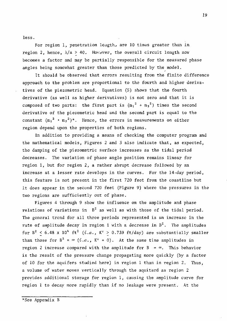
For region 1, penetration leJlgth., are 10 timC!s greater than in
region 2, hence, "A/a> 40. HOl·:c:ver, the overall circuit length now
becomes a factor and may be partially responsible for the measured phase
angles being somewhat greater than those predicted by the model.
19
It should be observed that errors resulting from the finite difference
approach to the problem are proportional to the fourth and higher deriva
tives of the piezometric head. Equation (5) shows that the fourth
derivative (as well as higher derivatives) is not zero and that it is
composed of two parts: the first part is (m1 2 + m3 2) times the second
derivative of the piezometric head and the second part is equal to the
constant (m1 2 • m3 2 )*. Hence, the errors in measurements on either
region depend upon the properties of both regions.
In addition to providing a means of checking the computer program and
the mathematical models, Figures 2 and 3 also indicate that, as expected,
the damping of the piezometric surface increases as the tidal period
decreases. The variation of phase angle position remains linear for
region 1, but for region 2, a rather abrupt decrease followed by an
increase at a lesser rate develops in the curves. For the l4-day period,
this feature is not present in the first 720 feet from the coastline but
it does appear in the second 720 feet (Figure 9) where the pressures in the
two regions are sufficiently out of phase.
Figures 4 through 9 show the influence on the amplitude and phase
relations of variations in 82 as well as with those of the tidal period.
The general trend for all three periods represented is an increase in the
rate of amplitude decay in region 1 with a decrease in 82• The amplitudes
for 82 < 6.48 X 10 4 ft 2 (i.e., K' > 0.739 ft/day) are substantially smaller
than those for 82 = 00 (i.e., K' = 0). At the same time amplitudes in
region 2 increase compared with the amplitude for 8 = 00. This behavior
is the result of the pressure change propagating more quickly (by a factor
of 10 for the aquifers studied here) in region 1 than in region 2. Thus,
a volume of water moves vertically through the aquitard as region 2
provides additional storage for region 1, causing the amplitude curve for
region 1 to decay more rapidly than if no leakage were present. At the
*See Appendix 8

20
same time, this volume of water causes the amplitude in region 2 to decay
at a lesser rate than it would if no aquitard were present. The fact that
the net decrease in the amplitudes of region 1 is so much larger than the
increases produced in region 2 is the result of having a storage coeffi
cient one hundred times greater in region 2 than in region 1.
The phase angle relations for region 1 remain essentially linear
except for B2 = 6.48 X 10 3 ft 2 (i.e., K' = 7.39 ft/day). There is an
apparent anomaly in the relative positions of the curves representing the
several values of B2 which is most noticeable in Figure 8 and to a lesser
degree in Figures 4 and 6. This can be explained in the following way.
The value of B2 = 00 represents the limiting case of ~wo separate infinite
aquifers, each with a phase angle which increases linearly with distance
from the coastline. The other limiting case occurs for B2 = 0, implying
that the region separating the two aquifers offers no resistance to flow.
In the latter limiting condition, the aquifer system would behave as a
single aquifer and the phase relation would essentially be determined by
the greater storage of region 2. This greater storage causes the phase
angle of region 1 to increase with respect to distance from the coastline
at a greater rate than it otherwise would. Confirmation of this fact is
provided by the data points representing B2 = 0 plotted in Figures 4, 5,
6, and 7. For values of B2 that are relatively small but not zero, this
effect on the phase angle is still quite noticeable for the longer period
tides (See Figure 8 where t = 14 days), since the responses of each aquifer
remain essentially in phase for some distance from the coastline. However,
as the tidal period decreases, the responses of the two aquifers experience
an increasing phase difference at any given distance from the coastline.
As a result of this greater phase difference the aquifer of region 1 uses
a decreased portion of the storage available in region 2. Thus, the phase
lag with respect to the coast in region 1 shows a subsequent decrease as
shown in Figures 4 and 6.
The most striking departure from the linear phase angle relation of
the infinitely long aquifer occurs in region 2 as shown in Figures 5, 7,
and 9. Here the phase angles follow closely the linear change for the
single aquifer for some distance from the coast and then decrease rapidly
(almost discontinuously for the larger values of B2) after which they

increase again. In several instances, a second set of maximum and
minimum points are present, but not to such extreme positions as the
ini tial set.
This sudden decrease of the phase angle in region 2 is caused by
water moving through the aquitard under a pressure gradient produced by
the more rapidly propagating tidal response in region 1. Hence, at that
distance from the coastline where significant flow through the aquitard
develops, the phase of region 1 is imposed on that of region 2 with the
resultant phase in the upper aquifer showing a decrease. For small
values of B2 this process repeats itself at a greater distance from the
coastline, producing a second set of maximum and minimum points (see
Figure 7).
21
It should be pointed out that the tidal periods used here are not
those of a real tide. However, any of the components of the semi-diurnal,
diurnal, or lunar fortnightly tides are adequately approximated by the .5,
O.S, 1, and 14 day periods, respectively.
CONCLUSIONS
From the results presented in Figures 2 through 9 and the preceding
discussion, it is evident that leakage can significantly influence tidal
response data from either of the two aquifers.
For the aquifer with the greatest storage, the deviations in the
phase angle are the most significant. However, these deviations take
place at a point where the amplitudes have decayed to 5 percent or less
of their initial value and phase angle measurements at such small amplitudes
may not be usable because of a lack of accuracy. The amplitudes seem to
be influenced less than the phase angles. However, for the range of
leakage values studied, they may be larger than those for no leakage by as
much as 100 percent for the l4-day period, 20 percent for the I-day period
and less than 20 percent for the O.S-day period.
For the aquifer with the least storage both the amplitude and the
phase angle values can be substantially different from those when no
leakage is present. The phase angles can be either larger or smaller than
those when no leakage occurs. The amplitudes are smaller than those when

22
there is no leakage and may be so by as much as an order of magnitude or
more for any of the three tidal periods considered. In general, the error
for both the phase angles and the amplitudes is smaller for larger values
of B2.
In view of these results, it is apparent that aquifer properties
based on tidal data may be completely erroneous if the data came from an
aquifer system where leakage was present as described above. Also, a
relatively moderate amount of leakage (1/B2 > 0.154 x 10- 4) can produce
errors of 100 percent or more for an aquifer system similar to the one
tested.
ACKNOWLEDGEMENTS
We would like to thank Dr. L.S. Lau and Dr. D.C. Cox for reviewing
and commenting on the manuscript and Dr. Giulio Venezian of the Department
of Ocean Engineering, University of Hawaii, for reviewing the mathematical
development.

23
REFERENCES
Karplus, W.J. 1958. Analog simulation. McGraw-Hill Book Company, Inc., New York.
McCraken, D.A. 1967. Fortran IV manual. John Wiley & Sons, Inc., New York, 4th printing.
McLachlan, N.W. 1934. Bessel functions for engineers. Oxford University Press, London.
Neuman, Gerhard and Willard Pierson. 1966. Principle of physical oceanography. Prentice Hall, Englewood Cliffs, New Jersey.
Sheddon, I.N. 1969. special functions of mathematical physics and chemistry. Oliver and Boyd, Edinburgh and London.
Walton, W.C. and T.A. Prickett. 1963. Hydrologic electric analog computers. ASCE Journal of Hydraulics Division. HY-6. p. 67-91.
Williams, John A. and Ta-Chiang Liu. 1971. The response to tidal fluctuations of two non-homogeneous coastal aquifer mode~s. Water Resources Research Center, University of Hawaii, Technical Report No. 51.

APPENDICES

a
AI, A2
bl, b2; b'
B. , J
Bl, B2
C 1, C2; C
e
h. , J
hI, h2
i
II, 12
Kl, •.• Kit;
L
illl, ••• , mit
p+ , p -P. ,
J PI, P2
Q
q+, q - ; q
s
t, t ; to e
x, z
A, B, C, D
K'
APPENDIX A. lIST OF SYMBOLS.
characteristic length, ft
complex constants
thickness of aquifer; of aquitard
the square root of the leakage factor, ft
complex constant; capacitance per unit of length, farads per grid spacing
base of natural logarithms
piezometric head, ft.
~ ; current, amperes
27
imaginary part of complex function for piezometric head
coefficient of permeability of aquifer, ft/day or scale factors for electric analog model; coefficient of permeability of aquitard ft/day
distance to coast from origin of coordinates
roots to fourth order characteristic equation
real parts of the roots to the characteristic equation
complex coefficients of basic differential equation
discharge, ft 3/sec
imaginary parts of the roots to the characteristic equation;' volume of water, ft 3
real part of complex function for piezometric head; resistance per unit length, ohms/grid spacing
aquifer storage
time, seconds, or days; tidal period, days
transmissivity, ft 2 /day or gal/day - ft
electrical potential, volts
space variables, ft or "a" feet units
constants of integration

28
2 R
CI.. , J
Cl.1,
(h, 02
£'
SO; S . , J
e p
A
(5
Cl.2
S1, S2
quantity of charge, coulombs
real part of
argument of complex roots to characteristic equations; argument of complex constant (P1 + P2)2 [(P 1 - P2)2 +
4/81 282 2]1/2
coefficient combining aquifer properties and tidal frequency, ft- 1
moduli of complex coefficients in the fourth order differential equations
effective porosity
amplitude of the tide at the coast; amplitude of piezometric surface
phase angle, degrees
penetration length - is the distance from the coastline to the point where fluctuations in the piez?metric head are in phase with the tide, i.e., (4T to/B) /2
modulus of complex roots to characteristic equation; dimensionless amplitude functions for region I and 2, respectively
angular frequency of tide, radians/sec
AQUIFER REGION 2
- 00 -.-i::: A '0 'tJ'(fA 'Rb:::::::::::::::::::::::::::::: ::::::::::: ::::: b I.~.: ~.: ~,: ~,: ~,: ~,: ~,: ~,: ~.: ~,: ~,: ~,: ~,:~ K I,: ~,,: ~.: ~.: ~,:~,: ~,: ~,: ~,: ~: ~: ~: ~ ~~: ~: ~: ~ ~ ~: ~ ~~ ~~ ~ ~ ~ ~ ~ ~: ................................................................................ COASTLINE
AQUIFER REGION I
x x = L
NOTE: REGION 2 MAY BE EITHER CONFINED FROM ABOVE OR PHREATIC, IN
THE LATTER CASE THE STORAGE EQUALS THE EFFECTIVE POROS ITY, 1
€ •
FIGURE A-I. DEFINING SKETCH FOR AQUIFER SYSTEM

29
APPENDIX B
Several special cases may be investigated by considering the
characteristic equation of (differential) equation (5). This characteristic
equation is
and ml, m2, m3, and m4 are the four roots given in equation (6). From the
theory of equations 2 + m3 2 PI + m~ =
ml 2 . m3 2 = PI P2
and therefore
(PI + P2) +-Y(PI - P2)2 + 4/B1 2B22
m1 2 = 2
m;l2 (PI + P2) --y (PI - P2)2 + 4/B12B22
= 2
The first case is that in which the aquitard becomes an aquiclude
i.e., K' approaches zero. Then I/BI 2 = I/B22= 0 and
The constants of integration in region 1 given by equations (lla) and (lIb)
become
-i/';o -i/';o =
i/';o i/';o =
Therefore, equation (12) reduces to
/';1 (x) = _i/,;0-jioa 1'(X-L) ,
which is the correct amplitude function for a single, one-dimensional
aquifer of infinite extent in region 1.

30
The constants of integration for region 2 can be calculated in a
similar fashion, i.e.,
where
B12C 2 C1
1 +' lim B12 (im)'.l-ml 2) = 0 K'+O
= + B12(iaal-m32)--------m12-m32 m12-m32
o + lim B12(iaal-m12) = -1 K'+O
=
= -1 K'+O K'+O
since m1 2+Pl as K'+O. Equation (14) becomes
i;;dx) = ii;;o&/iaa2 i (x-L)
which is the correct amplitude function for a single, one-dimensional
aquifer of infinite extent in region 2.
The second case is that in which both aquifers are identical. Then
and
m1 2 = P + 1/B 2
This gives, for region 1
Al iaa -P + 1/B2 = = 0,
C1 iaa- P - 1/B2 = -1

and
Similarly, for region 2
and
. r -:Yicr(J,' (x-L) -l~oe .
2 2 mI -m3
=
=
82
2
mI
Al
CI
2 -m3
7;2(X) = . r Vicr(J,' (x-L) -l~oe
31
= 0,
= -1 2

APPENDIX C
Computer program and print-out for mathematical model of leaky aquifer
system:
to = 0.5 day
8 2 = 6.48 x 10~ ft 2
Tl = T2 = 1330 ft 2 /day
Sl = 0.002
S2 = 0.2
33

34
I IV G LEVEL 20 MhIN DATE = 73011 1215C;13f:
C LEAKY AQUIFER - REGION 1 (CCNFINEDJ C AL = AQUIFER LENGTH (FEET) C PERIOD = TIDAL PERIOD (HOURS) C B = AQUIFER THICKNESS (FEET) C CK = HYDRAULIC CCNCUCTIVITY (FT.IDAY) C S = STORAGE COEFFICIENT C BSQRT = LEAKAGE FAtTeR (FT.**2)
DOUbLE PRECISION CK3,PERIOO,AL,CKJ,CK2,Bl,B2,Sl,52,Tl,T2,B3,SIG~A, 1 ALPHA1,ALPHA2,COl,C02,B,A,RHCl,Z,BD} ,ZPl,ZP2,RH02P,RhC2,lP, 2 B02p,B02,BMl,BM2,B~3,BM,RHOP,RHCM,PP,P~,QP,QM,A1R,A1I,CIR,
3 C1I,TENX,X,PPXL,PMXL,QPXL,Q~XL,AIX,AIL,ARX,ARL,RI1,RI2,RIL, 4 BP1,BP2,BP3,BP,RHO,TAM,THETA,DEGREE,CP,CM,D,BSQRT
10 READ(5,1,END=30)AL,Bl,B2,B3,Sl,S2,CKl,CK2,CK3,PERIOO 1 FOR~ATIF7.0,7F6.0,2Fl0.0)
BSQRT = (CK1*Sl*e3)/CK3 W~ITE(6,lOO)AL,PERIOD,Bl,CKl,B2,CK2,B3,CK3,Sl,S2,85CRT
100 FOPMAT(lHl,'AL = I,F7.l,' FT',5X, 'PERIOD = ',F12.3,' HRS'/IHO, 1 'Bl = ',F7.1,' FT',5X,'CKl = ',FI2.3,' FT/DAY'/IHO,'B2 = " 2 F7.1,' FT',5X,'CK2 = ',FI2.3,' FT/DAY'/IHO,'B3 = ',F7.l, 3 • FT',5X,'CK3 = ',Fl2.6,' FT/DAY'/IH~,'SI = ',F7.5,8X, 4 '52 = ',F1.5/1HO,'BSQRT = ',lPOll.5,· FT**2')
PERIOD = PERICD*3600.0 CK) = CKl/8640C.O CK2 = CK2/8640C.0 CK3 = CK3/86400.0 Tl = CKl*Bl T2 = CK2*B2 SIGMA = 6.2831853/PfRICD AL PHAl = S I/Tl ALPHA2 = S2IT2 WRITF((;,4)
4 FORMAT(111HO, 'LOCATION',6X,'AMPLITUOE',9X,'PHASE ANGLE'/) CBl = CSQRT«CK1*Bl*e3J/CK31 CB2 = CSWRTI(CK2*B2*B3UCK31 B = SIGMA*(ALP~Al+~LPHA2) A = (1.0/(CR1**21)+ll.O/(CB2**2)) RHGl = DSQRT(A**2+B**2) Z = EI A BD] = DATANIZ) IF (8 .GT. 0.0 .AND. A .LT. 0.0) BD1 = B01+3.14]5921 IF (6 .LT. 0.0 .ANC. A .LT. 0.0) BOl = 801+3.1415927 IF 18 .LT. 0.0 .ANC. A .GT. 0.0) BCI = BCl+6~2831853 CP = (1.0/ICB1**2»+11.0/(CB2**2») CM = 11.0/(C61**2»"-(1..0/(C82**2» o = SIGMA*(~LPrAI-ALPHA2) ZPl = 2.0*CfA*O ZP2 = CP**2-0**Z RH02P = DSC~T(lP2**2+lPl**2)

35
, IV G LEVEL 20 MAIN DATE .. 73011 12159/36
RHC2 ; DSQRT(R~02P)
IP = IPI/ZP2 BD2P = DATAN(ZPJ IF HPI .GT. 0.0 .AND. ZP2 .LT. O.C) BD2P" AC2P+3.1415921 IF (IPI .LT. 0.0 .AND. ZP2 .LT. 0.0) BD2P = BD2P+3.~415921 IF (ZPI .LT. 0.0 .AND. ZP2 .GT. 0.0) BD2P : B02P+6.2831853 tW2 = B02PIZ.O BPI = RHOl*OSIN(BDl)+RhC2*DSIN(BDZ) BP2 = RHOl*OCCS(BOl)+RHOZ*OCOS(B02) BP3 = BPI/BP2 BP = DATt>N(BP3) IF (BPl .GT. 0.0 .AND. BP2 .LT. 0.0) BP = BP+3.1415927 IF (SPI .LT. 0.0 .AND. BP2 .LT. 0.0) BP = BP+3.J4IS921 IF (BP1 .• LI. 0.0 .AND. BP2 .GT. 0.0) BP = BP+6.2831853 BMI = RH01*OSI~(BOl) - RH02*OSIN(BC2) BM2 = RHOl*CCOS(BOlJ - RH02*OCOS(BDZ) BPl3 = BMI/BMZ BM = OAIAN(BM3) IF (BMI .GT. 0.0 .AND. BM2 .LT. 0.0) BM z B~+3.1415927 IF (BMI .LT. 0.0 .A~D. BM2 .LT. 0.0) 8M = BM+3.1415921 IF (BMI .LT. 0.0 .AND. 8M2 .GT. 0.0) 8M : BM+6.2831853 RHOP = DSQRT(RHOl**Z+RH02**2+2.0*R~Cl*RH02*DCCS(BDl-B02»/2.0 RHOfol = DSQRT(RHOl*~2+RH02*¥Z-2.0*RHCI*RH02*DCOS(BDl-BD2»/2.Q PP = (DSQRT(R~CP»*OCOS(BP/2.0) p~ = (OSQRT(RHCM)I*DCOS(B~/2.0) OP = (DSCRT(R~CP»*DSIN(BP/2.01 OM : (DSO~T(R~CMI}*DSIN(BfoII2.0)
AIR = QM**2-P~**2 All = SIGMA*ALPHAl-2.0*PM*CM CIR .. (-1.0)*(~P**2-PP**2' C11 s (-1.0)*(SIGMA*AlPHAl-2.0*PP*~P)
TENX = 20.0 20 X .. TE~X/20.0
PPXL .. PP*(X-l.O)*AL PMXL .. PM*(X-l.O,*AL QPXl .. QP*(X-l.O)*AL QMXL .. QM*(X-l.O)*AL AIX .. (AIR*OSIN(OPXl)+AII*OCOS(QPXL)'*OEXP(PPXL)
~ +(CIR*DSIN(QMXl)+CII*DCOS(QMXL»)*DEX~(PMXl)
All .. AI I+C1 I ARX .. (AIR*DCOS(QPXL)-AII*CSIN(QPXL»)*DEX~(~~XL)
7 +(Cl~.OCGS(QMXL)-Cl[.CSIN(OMXL))*OEX~(~MXL) ARL .. A1~+Clfit
ill • AIL*AIX + ARL*A~X RI2 • -AIL*A~X + A~L*AJX RHO • DSQRT«(A~X**2+AIX.*2)/(A~l**2+AIl*.Z)
TA~ • 1I12lRIl THETA .. DATAN(TAM)

36
j IV G LEVEL 20 MAIN DATE = 73011 12/!S9/36
IF IR12 eGT. 0.0 .AND. RII .LT. 0.0) THETA = THfTA-3.14)5927 IF IRI2 .LT. 0.0 .ANC. RII .LT. 0.01 THETA = THETA-3.1415927 DEGREE = THfTA*360.0/6.2831853 WRITE (6,31 X, RHO, CEGREE
3 FORMATIIHO,09.3,2X,Dl5.6,3X,D16.6) IF (X .LE. l.e) GO TO 10 TENX = TFf'.<X-l.C GO Te 20
30 CALL EXIT ENe

37
AL .: 72u.0 FT PERIOD = 12.000 HRS
B1 = 100.0 fT CK1 = 13.300 fT 10 A 'I'
B2 = 50.0 fT CK2 = 26.WO FT 10AY
B3 = 36.0 fT (K3 = 0.738900 FT/OAY
Sl = 0.00200 52 = 0.20000
BSQRT = 6.479900 04 FT**2
LOCATION AMPLITUDE PHASE ANGLE
0.1000 01 0.1000(00 01 O.C
(.9500 00 0 •. 8538C40 00 -O.4766E:5O 01
0.9000 00 0.7257860 CO -0.'1286430 01
C.8500 00 0.6172'>00 00 -0.1367320 02
0.8000 00 0.5254730 OC -0.1804330 C2
0.7500 00 0.4474340 00 -0 •. 2242660 02
0.7000 00 0.3809770 CO -0.2681780 02
0.6500 00 0.3243740 OC -0.~12100D 02
0.6000 00 0.2761 770 00 -0.3560160 02
0.5500 00 0.2351410 ('0 -,0.3999270 02
C.500D 00 0.2002C30 00 -0.4438380 02
0.4500 00 0.1704570 00 -0.4877490 02
0.4000 00 0.1451300 00 -0.5316HO 02
0.3500 00 0.1235 t60 CO ~o. 5755 710 C2
0.3000 00 0.1052060 00 "0.61'14820 C2
0.25UO (,0 0 •. 8957450- 01 ··O.H33'130 02
C.200D 00 0.7626530-01 -0.7073 C40 02
0.1500 00 0.6493360-01 -0.7512150 02
0.100D 00 0.5528570-01 -0.795126C 02
0.5000-01 0.470n2o-01 ·-0.8390370 02
0.0 0.400772D-01 -0.8829 Lr90 02

38
IV G LEVEl 20 MAIN DATE = 73011 13/01/25
C LEAKY AQUIFER - REGICN 2 (PrREATIC) C AL = A~UIFER LENGTH (FEET) C PERIOD = TIDAL PERIOD (HOURS) C B = AQUIFER THICKNESS (FEET) C CK = HYDRAuLIC CCNCUCTIVITY (FT./DAY) C S = STCRAGE CCEFFICIENT C BSQRT = LEAKAGE FACTeR (FT.**2)
oouelE PRECISICN CK3,PERIOD,AL,CK1,CK2,BI,B2,Sl,S2,TJ,T2,B3tSIG~A, 1 AlPHAI,~LPHA2,C81,CB2,B,A,RH01,Z,BD1,ZPl,ZP2,RH02P,RHO 2,lP,
2 BD2p,eC2,eMl,eM2,B~3,BM,RHOP,RHCM,PP,P~,QR,C~,AlR,AlI,CJP,
3 CII,TE~X,X,PPXL,PMXL,OPXL,Q~XL,AIX,AIL,ARX,ARL,RI1,RI2,RIL, 4 BP1gep2,EP3,8p,RrO,TAM,THcTA,CEGREE,CP,C~,O,XX,yy,BSQRT
10 REAO(5,l,ENO=3C)AL,Bl,B2,B3,Sl,S2,CKl,CK2,CK3,PERICD 1 FOR~'T(F7.0,7FfoO,2F10.0)
BSQRT = (CK2*B2*B3)/CK3 WRITE(6,100IAL,PERIOD,81,CKI,B2,CK2,B3,CK3,SJ ,S2,BSQRT
100 FOP"'ATUHl,'Al::: I,F7.1,' FT',5X,'PERIOD = ',F12.3,' HRS'/lHO, 1 'B1 = I ,F7.1,' FT',5X,'CK1 :: ',F12.3,· FT/DAY'/lHO,'B2 = " 2 F7.l,' FT',5X,'CK2 = ',F12.3,' FT/DAY'/lHO,'B3 = ',F7.l, 3 ' FT',5X,'CK3 :: ',FI2.6,' FT/CAY'/IHO,'Sl = ',F7.5,8X, 4 'S2:: ',F7.5IlHQ,'BSQRT :: ',IPOII.5,· FT**2,)
PERIOD = PERICC*3600.0 CKI = CKl/8640CeO CK2 = CK2/864CC.O CK3 :: CK3/8640C.O Tl = CKl*BI T2 = CK2*B2 SIGMA = 6.283l853/PERICC ALPHAl = SlITl ALPhA2 :: S21T2 WRITE(6,41
4 FOR~AT(I/1H0,'LCCATICN',6X,'AMPLITUCE',9X,'PHASE ANGLE'/) C81 = CSQRTI(CK1*BI*B3)/CK3) CB2 = CSQRT«CK2*82*B3)/CK3) B = SIGMA*(ALPhA1+~LPHA2) A = (1.0/(C81**21)+(1.C/(CB2**2» RHCl :: OSQRT(A**2+8**2) l :: 8/A BCI = CATANlz) IF IB .GT. 0.0 .ANC. A .LT. 0.0) BCI ~ 8Cl+3.1415927 IF (8 .LT. O.C .ANO. A .LT. 0.0) BDI = B01+3.1415927 IF (B .LT. 0.0 .AND. A .GT. O.O) BCl = BD1+6.2831E53 CP = (1.C/(CB2**2) )+(1.0/(C81**2» eM = o..0/(C82**2) )-0.0/(C81**2» o = SIGMA*(ALFhA2-~LPHAll lPl = 2.')*0'*0 lP2 = CP**2-C**2 RH02P :: DS~RT(ZP2**2+lF]**2)

39
IV G LEVEL 20 MAIN DATE = 73011 13/01/25
RHC2 = DSCRTlRr02P) ZP = ZPIllP2 BD2P = DAHNl lP) IF (ZPI .GT. 0.0 IF lZPI .LT. 0.0 IF (Z P 1 .LT. 0.0 BD2 = BD2P/2.0
.ANC. ZP2 .LT. 0.0) B02P =
.AND. ZP2 .LT. 0.e) B02P =
.AND. ZP2 .GT. 0.0) BD2P =
BC2P+3.1415927 BC2P+3.1415927 B02P+6.2831853
BPI = RHOl*DSI~(BDI)+RH02*DSIN(BD2) BP2 = RH01*CCCS(BDIJ+RhC2*DCOS(BD2) BP3 = BPI/BP2 BP = DATAN(BP3) IF (BPi .GT. 0.0 .AND. BP2 .LT. 0.0) BP = IF (BPI .LT. 0.0 .AND. BP2 .LT. 0.0) 8P = IF (BPI .LT. 0.0 .AND. BP2 .GT. D.C) BP = BMI = RH01*DSI~(BDII - RH02*DSIN(BC2J 6M2 = RHOI*CCOS(BDIJ - RH02*DCOS(BC2) Bn :: BMlIBt-'2 B/ol = DATAN(BM3)
BP~3.1415927
BP+3.14I5927 BP+6.2831853
IF (BMI .GT. c.a .AND. BM2 .IT. 0.0) BM = B~+3.I415927 IF (BMI .IT. 0.0 .AND. BM2 .IT. 0.0) BM = BM+3.1415927 IF (BMl .IT. 0.0 .ANC. BM2 .GT. O.O) BM = BM+6.2831853 RHOP = DSQRT(RHOI**2+RHC2**2+2.0*RHCl*RHC2*DCCS(BDl-B02)}/2.0 RHeM = DSQRT(RhOl**2+RH02**2-2.0*RhDI*RH02*DCCS(BDl-B02»)/2.0 PP = (OSQRT(RhCP»*OCOS(BP/2.0) PM = (OSQRT(RHC~)}*OCOS(BM/2.0) OP = (OSCRT(RhCP»*OSI~lBP/2.0) OM = (DSQRT(RHC~»*OSIN(BM/2.0) AIR = (QM**2-P~*~2)*«1.0/cel**?I-PP**2+QP**2)-(SIG~A*AlPHA1-
6 2.0*FM*CtJ)*(SIGMA*ALprAl-2.0*PP*QP» All = ((I.O/CBl**2)-PP**2+QP**2)*(SIG~A*AlPHAl-2.0*PM*CM)+
7 «(SIGMA*AlPHAl-2.G*PP*QP)*(Q~**2-PM**2)} , CIR = (PP**2-'P**2)*«1.0/cel**2)-P~**2+0M**2}+«SIGMA*AlPHAI-S 2.0*PP*CP)*lSIGMA*4LPhAl-2.0"PM*CM)) GIL = (-1.0)*«ll.O/CB1**2)-PM**2+0~**2)*(SIG~A*AlPHA!-
~ 2.0*PP*CP)+( (QP**2-PP**2)*(SlGMA*ALPHAl-2.0*PM*QM»)) TENX = 20.0
20 X = THX/20.0 PPXl = PP*(X-l.O)*Al P~Xl = P~*(X-l.O)*Al QPXL = CP*(X-l.O)*AL Q~Xl = O~*(X-l.G)*AL AIX = (AIR*OSI~(OPXl)+AII~OCOS(QPXL})*DEXP(PPXl)
6 +(CIR*DSI~(CMXl)+CII*OCOS(QMXl»*DEXP(PMXl) AIL = AlI+ClI ARX = (AIR*OCCS(QPXL)-AII*CSIN(QPXl»)*OEXP(PPXl)
7 +(CIR*~CCS(QMXl)-CII*CSI~(Q~Xl))*DEXP(PMXl) ARl = AIR+C1R XX = (PP**2-'P**2)-(PM*~2-CtJ**2)

40
IV G LEVEL 20 MAIN DATE = 73011 13/01/25
VV = 2.0*(PF*CF-PM*C~' RI2 :: AIX*XX-APX*VY RII AKX*XX+AIX*VV RHO:: (CBl**Z)*(OSCRT( (ARX**Z+AIX**2)/(XX**2+YV**2))) TA~ = RI2IRll THETA :: DATAN(TA~)
IF (RIZ .LT. 0.0 .AND. RIl .LT. 0.0) T~[TA :: THETA-3.1415927 IF (RI2 .GT. O.G .AND. RIl .LT. 0.0) THETA THETA-3.l415927 DEGREE = TrETA*3cO.0/6.2831e53 WRITE (6,3) X, RHO, CEGREE
3 FORMATIIHO,D9.3,ZX,D15.c,3X,016.6) IF (X .LE. O.OJ GO Te 10 TENX = HNX-l. C GO Te 20
30 CALL EXIT END

41
AL :: 72U.O FT PE R 1.00 :: 12.000 HRS
B1 ... 100.0 FT CK1 :: 13.300 FT 10AY
B2 .. 50.0 FT CK2 :: 26.l:00 FT IOA't
83 = 36.0 FT CK3 :: 0.738900 FT IOA't
51 = 0.00200 S2 :: 0.20000
BSQRT = 6.479<;00 04 FT**2
LOCATION AMPLI HOE PHASE AI\GlE
0.1000 01 0.1000COO 01 0.3802300-15
0.9500 00 0.3352C90 CO - o. l: 3 30 l: 4 [j 02
0.9000 00 0.1l31l:20 CO -0.1244580 03
0.850D 00 0.3644190-01 -0.1809450 03
0.8000 VO 0.8612730-02 -0.2349640 C3
0.7500 00 0.1512850-02 -0.2723210 C2
0.7000 00 0.3215960-02 -0.9362650 02
0.6500 00 0.3010940-02 .<, 0.1159920 03
0.6000 00 0.2409100-02 -0.1265480 03
0.5500 00 0.1949840-02 -0.1311l:60 03
0.5000 00 0.1640710-C2 -0.1346100 03
0.4500 00 0.1401470-02 -0.1385890 03
0.4000 00 0.1196840-02 -0.1429590 03
0.3500 00 0.1019750-02 -0.1474030 03
0.3000 00 0.8680940-03 -0.1518180 C3
0.2500 00 0.738983D-C3 -0.15l:21l0 03
0.2000 00 0.6291550-q3 -0.1606000 03
0.1500 00 0.5356780-03 -0.1649890 03
(.1000 00 0.4560<;00-03 -0.16«;3800 03
O.5000-ul 0.3883240-03 -0.1737120 C3
0.0 O. 3 306 2 6 0- 03 -·0.1781l:3D 03