1/10/20071 APHEO: Longitudinal Data Analysis; Overview and Conceptual Ideas October 15, 2007 Dr. N. Birkett, Department of Epidemiology & Community Medicine,

1/10/2007 1

APHEO:Longitudinal Data Analysis;

Overview and Conceptual IdeasOctober 15, 2007

Dr. N. Birkett,Department of Epidemiology &

Community Medicine,University of Ottawa

1/10/2007 2

Overview

• What is longitudinal analysis?

• Data structure

• Graphical approaches

• Analytical methods– Multi-level model– Growth curves

• Emphasis on examples, not mathematics

1/10/2007 3

Intro (1)

• Poverty in Canada– Survey of Labour and Income Dynamics (SLID)

• Statistics Canada (1993-1996)

Poverty Rate, Canada

Year

1993 1994 1995 1996

Per

cent

0

2

4

6

8

10

12

14

1/10/2007 4

Intro(2)

• Poverty percent seems fairly constant– Slight increase but always around 12%

• Interpretation– There is a group of people in Canada who live

in constant poverty– There are many people who live in poverty for

parts of their lives.

• Very different policy implications

1/10/2007 5

Intro(3)

• How to tell these situations apart?

• Need within-subject data over multiple years (time points)– Panel survey– cohort study– Etc.

1/10/2007 6

Intro (4)

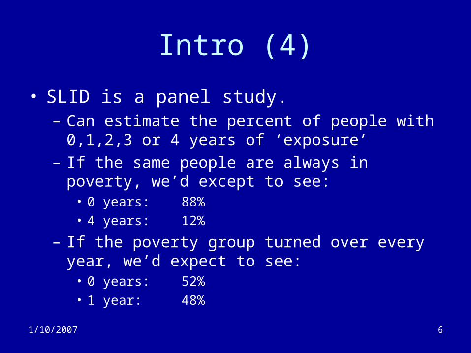
• SLID is a panel study.– Can estimate the percent of people with 0,1,2,3 or 4

years of ‘exposure’– If the same people are always in poverty, we’d except

to see:• 0 years: 88%• 4 years: 12%

– If the poverty group turned over every year, we’d expect to see:

• 0 years: 52%• 1 year: 48%

1/10/2007 7

Intro(5)

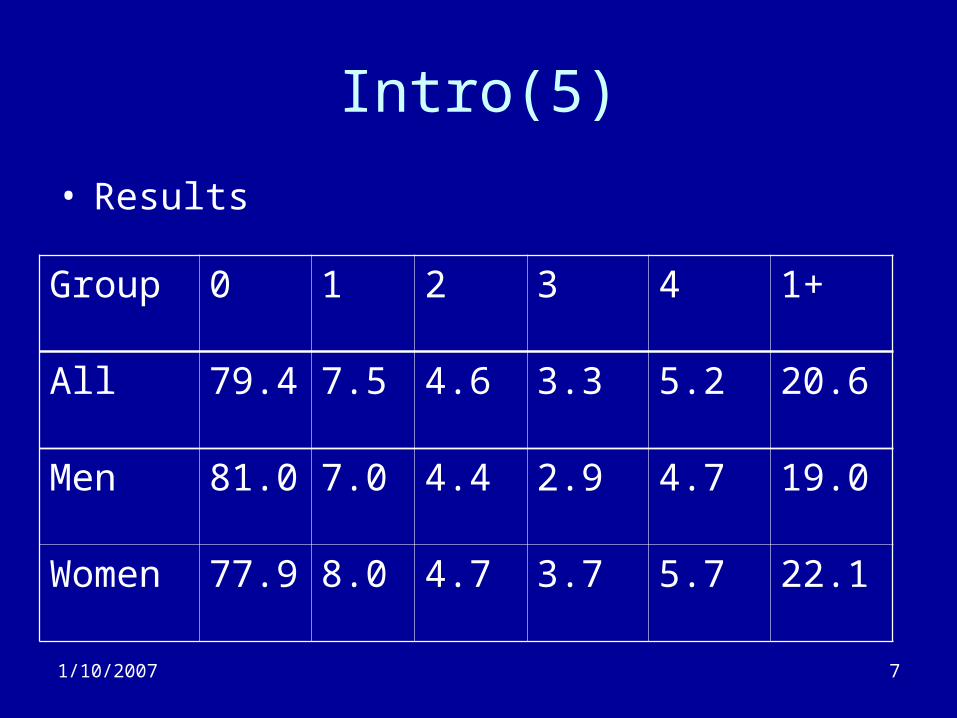
• Results

Group 0 1 2 3 4 1+

All 79.4 7.5 4.6 3.3 5.2 20.6

Men 81.0 7.0 4.4 2.9 4.7 19.0

Women 77.9 8.0 4.7 3.7 5.7 22.1

1/10/2007 8

Intro(6)

• Panel data shows– Poverty affects more people than suggested

by the cross-sectional prevalence– Few people are exposed to constant poverty– Suggests need for policy interventions to

keep people out of poverty more than to get them out of poverty

1/10/2007 9

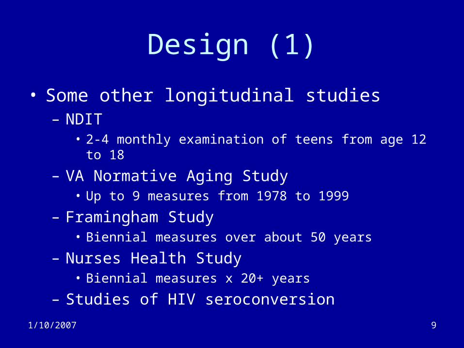
Design (1)

• Some other longitudinal studies– NDIT

• 2-4 monthly examination of teens from age 12 to 18

– VA Normative Aging Study• Up to 9 measures from 1978 to 1999

– Framingham Study• Biennial measures over about 50 years

– Nurses Health Study• Biennial measures x 20+ years

– Studies of HIV seroconversion

1/10/2007 10

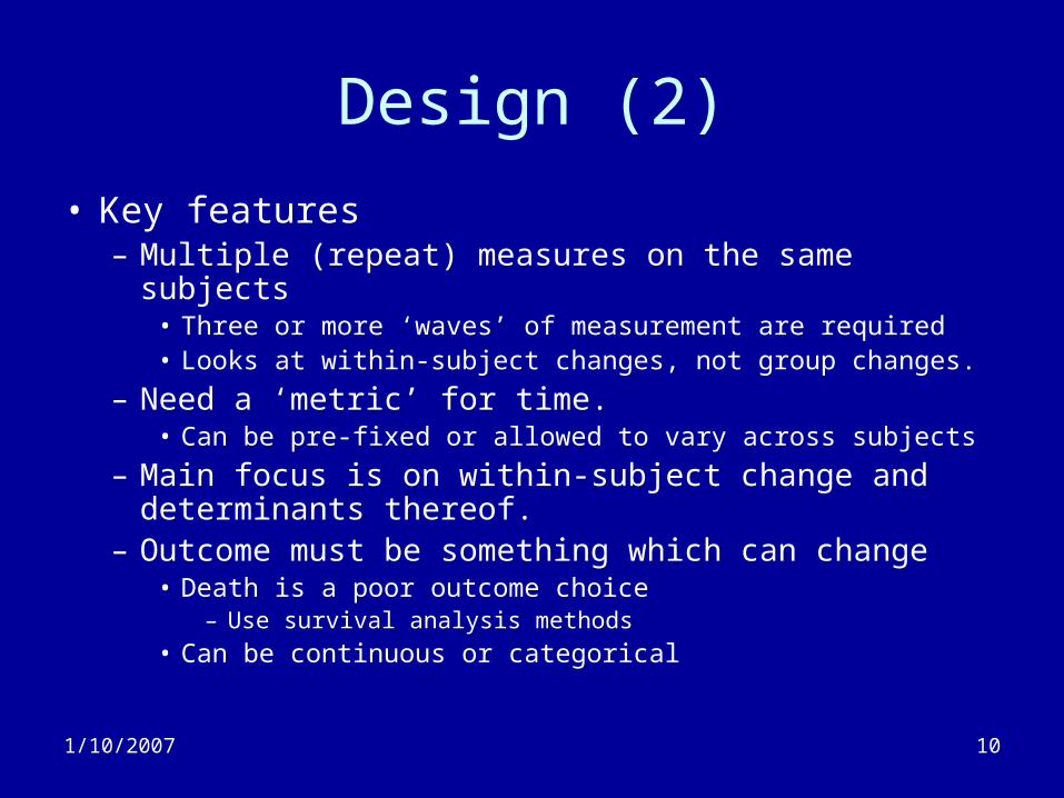
Design (2)

• Key features– Multiple (repeat) measures on the same subjects

• Three or more ‘waves’ of measurement are required• Looks at within-subject changes, not group changes.

– Need a ‘metric’ for time.• Can be pre-fixed or allowed to vary across subjects

– Main focus is on within-subject change and determinants thereof.

– Outcome must be something which can change• Death is a poor outcome choice

– Use survival analysis methods

• Can be continuous or categorical

1/10/2007 11

Design (3)

• Data structure– Normal approach for data is to define one

record per subject (Broad/person-level)• If subjects have measures at more than one time,

define two or more variables:– Smoke1, smoke2, smok3

– Longitudinal analysis needs a different layout: Long/person-period

• One record per time point per subject.

1/10/2007 12

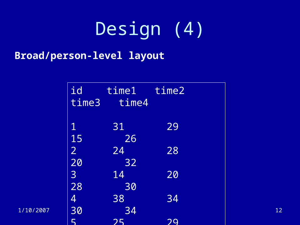
Design (4)

id time1 time2 time3 time4

1 31 29 15 262 24 28 20 323 14 20 28 304 38 34 30 345 25 29 25 296 30 28 16 34

Broad/person-level layout

1/10/2007 13

Design (5)Long/Person-period layout

id time score

1 1 311 2 291 3 15

1 4 262 1 242 2 282 3 202 4 323 1 143 2 203 3 283 4 30

id time score

4 1 38

4 2 344 3 304 4 345 1 255 2 295 3 255 4 296 1 306 2 286 3 166 4 34

1/10/2007 14

Analysis approaches

• Exploratory data analyses are common– Graphical methods– Trajectories

• Hypothesis testing• Model building• Identification of ‘latent classes’

– Unknown groups which show similar trajectories within group but different among groups

1/10/2007 15

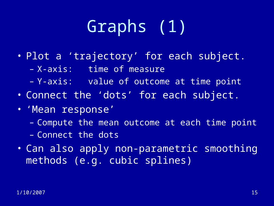
Graphs (1)

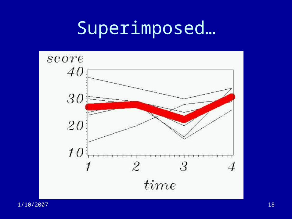
• Plot a ‘trajectory’ for each subject.– X-axis: time of measure– Y-axis: value of outcome at time point

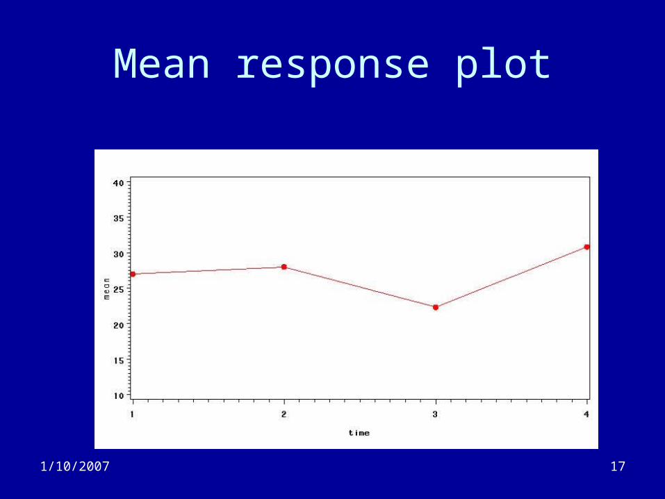
• Connect the ‘dots’ for each subject.• ‘Mean response’

– Compute the mean outcome at each time point– Connect the dots

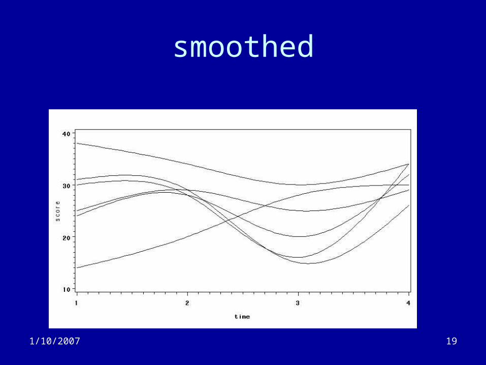
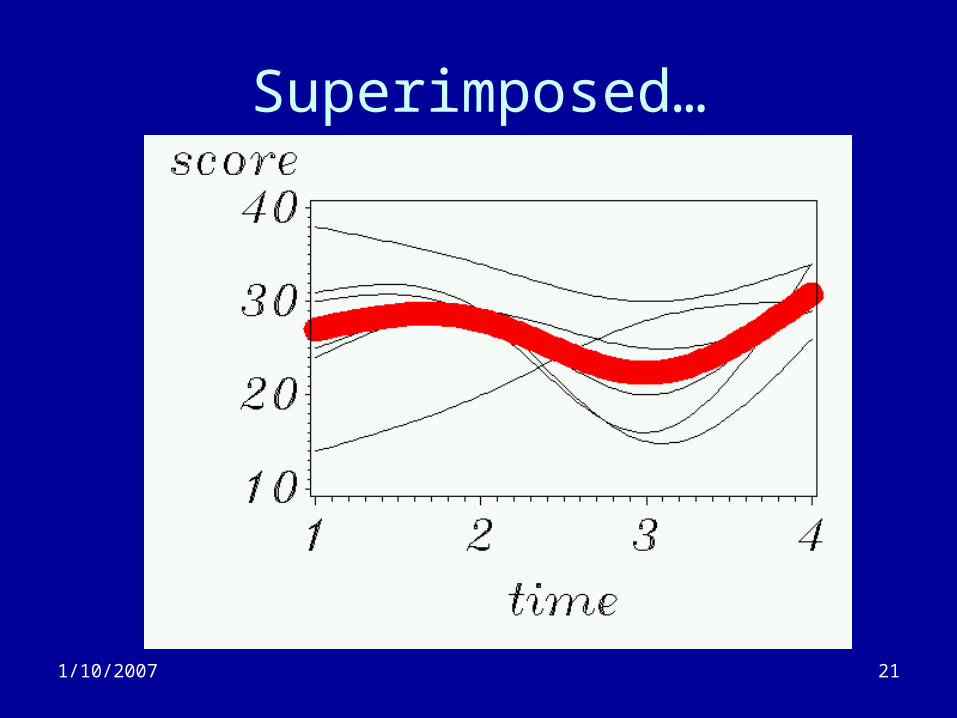
• Can also apply non-parametric smoothing methods (e.g. cubic splines)

1/10/2007 16

Profile plots (use long form)

1/10/2007 17

Mean response plot

1/10/2007 18

Superimposed…

1/10/2007 19

smoothed

1/10/2007 20

smoothed

1/10/2007 21

Superimposed…

1/10/2007 22

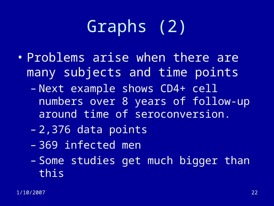
Graphs (2)

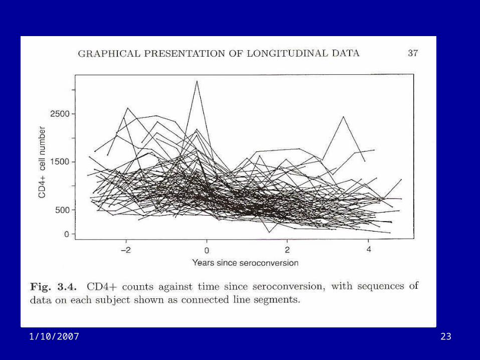
• Problems arise when there are many subjects and time points– Next example shows CD4+ cell numbers over

8 years of follow-up around time of seroconversion.

– 2,376 data points– 369 infected men– Some studies get much bigger than this

1/10/2007 23

1/10/2007 24

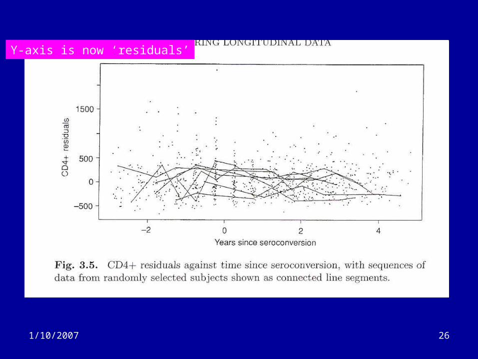
Graphs (3)

• Very busy graph• Not too useful

– ‘Except from the perspective of an ink manufacturer’

• Options

– Fit mean response only (LOESS smooth)• Ignores within subject changes

– Plot random sub-set of subjects• Arbitrary selection

– Plot subjects based on percentile of overall response

1/10/2007 25

1/10/2007 26

Y-axis is now ‘residuals’

1/10/2007 27

1/10/2007 28

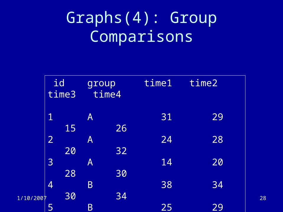
Graphs(4): Group Comparisons

id group time1 time2 time3 time4

1 A 31 29 15 262 A 24 28 20 323 A 14 20 28 304 B 38 34 30 345 B 25 29 25 296 B 30 28 16 34

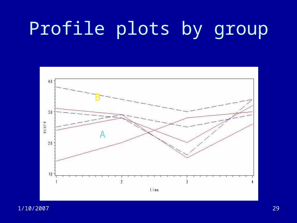
1/10/2007 29

Profile plots by group

B

A

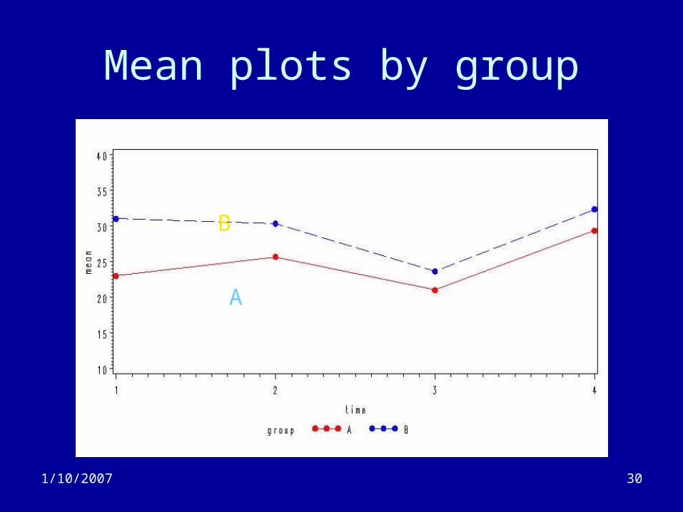
1/10/2007 30

Mean plots by group

B

A

1/10/2007 31

Types of questions you might ask

• What is the pattern of change over time?• Are there significant changes from baseline?• Do all people show the same trajectories?• If not, are there factors associated with different

trajectories?• In a two group comparison, do the two groups

differ in their responses over time?• Do the two groups differ at any time points?

1/10/2007 32

Analytic Strategies (1)

• T-test at final time point• ANCOVA at final time point• ANOVA using wave as factor

– Could use multiple comparison methods (e.g. Tukey’s test) to look for wave specific differences.

• MANOVA• Regression models (Ordinary Least Squares)

– Uses the time point as an ‘x’ variable to model overall trajectory for study group

– Ignores within subject change; looks at group mean changes– Can model non-linear predictors and multiple predictors.

1/10/2007 33


• Previous methods all suffer a serious weakness– They ignore the with-in subject change (except

ANCOVA).– Assumes that each subject has the same trajectory– Ignores the correlation between measures on the

same subject at different time points• Variance estimates and significance are biased.

– Tests at final time point ignore intermediate results which could be of value in programme design.

1/10/2007 34


• Change scores

• Repeated Measures ANOVA

• Random coefficient models

• Multilevel Model of Change

• Growth Models

• Latent class growth models

1/10/2007 35


• Simple within subject trajectory analysis– Perform separate OLS regression models for

each subject• For linear model, gives one intercept and one

slope for each subject.

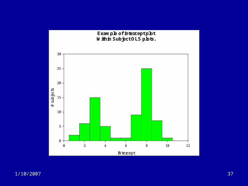
– If subjects follow different trajectories, than the distribution of the betas will show a pattern

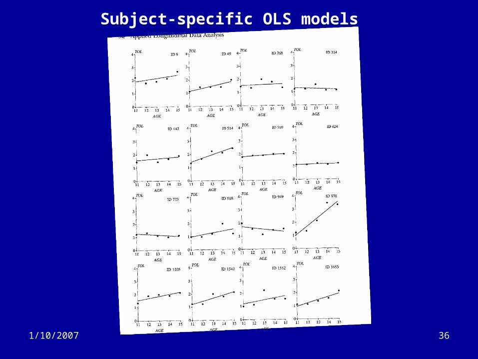
1/10/2007 36

Subject-specific OLS models

1/10/2007 37

Example of intercept plotWithin Subject OLS plots.

INtercept

0 2 4 6 8 10 12

# s

ub

ject

s

0

5

10

15

20

25

30

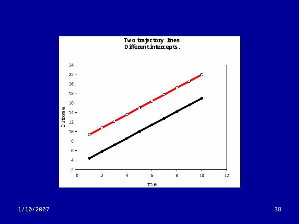
1/10/2007 38

Two trajectory linesDifferent intercepts.

time

0 2 4 6 8 10 12

Ou

tcom

e

2

4

6

8

10

12

14

16

18

20

22

24

1/10/2007 39

Multilevel model of change (1)

• Standard OLS regression model is:

ijijij timey *10

• Betas are assumed to be fixed. That is, there is a single common trajectory for ALL subjects.

• An departure from this predicted/expected trajectory is due to random variation (or unmeasured predictors) and shows up in the error term.

1/10/2007 40


• In my previous example, betas are NOT the same for each subject.

• If we had a predictor (e.g. sex), we could model it directly by adding a sex term (or a time*sex interaction if the slope varied).

• Predictors may be unknown.• Multilevel model of change allows the betas to

be RANDOM VARIABLES, not fixed.• Allows modeling of measured predictors

1/10/2007 41


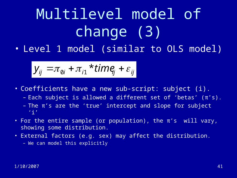
• Level 1 model (similar to OLS model)

ijijiiij timey *10

• Coefficients have a new sub-script: subject (i).– Each subject is allowed a different set of ‘betas’ (π’s).– The π’s are the ‘true’ intercept and slope for subject ‘i’

• For the entire sample (or population), the π’s will vary, showing some distribution.

• External factors (e.g. sex) may affect the distribution.– We can model this explicitly

1/10/2007 42


• Level 2 model (models the coefficients at level 1)

iii

iii

Sex

Sex

111101

001000

*

*

• The ζ’s follows a bivariate normal distribution with means ‘0’.

• These models can be made more complex– Add additional functions of time for the trajectory– Add additional level 2 predictors.

1/10/2007 43


• Model can be fit using– Multilevel software package– Mixed-model methods

• Output includes the ‘normal’ fixed effect model (the ‘best’ trajectory fitting all of the data)

• Estimates of the extent of variation in the random component– Large values suggest the need for more predictors

• Variances, etc. reflect within subject effects and correlations

• Can model correlation more explicitly (GEE methods)• Does not require time points to be evenly spaced

1/10/2007 44

Latent Class Growth Models

• Similar modeling approaches as multi-level methods

• Assumes that there are distinct ‘classes’ of trajectories but we don’t know which people belong to which class (or why)

• Fits the ‘best’ model with the pre-specified number of classes

• Explore classes for potential predictors, differences, etc.

1/10/2007 45

Application (1)

• Smoking onset in teens• McGill Natural History of Nicotine Dependence

(NDIT)– PI: Dr. J. O’Loughlin– Published in Ann Epidemiol, 2005

• 1,293 grade 7 students– 369 ‘novice’ smokers with 3+ measures

• Followed every 3-4 months for 3.5 years• Main outcome: smoking intensity

– Estimate of # of cigarettes smoked in previous 3 months

1/10/2007 46

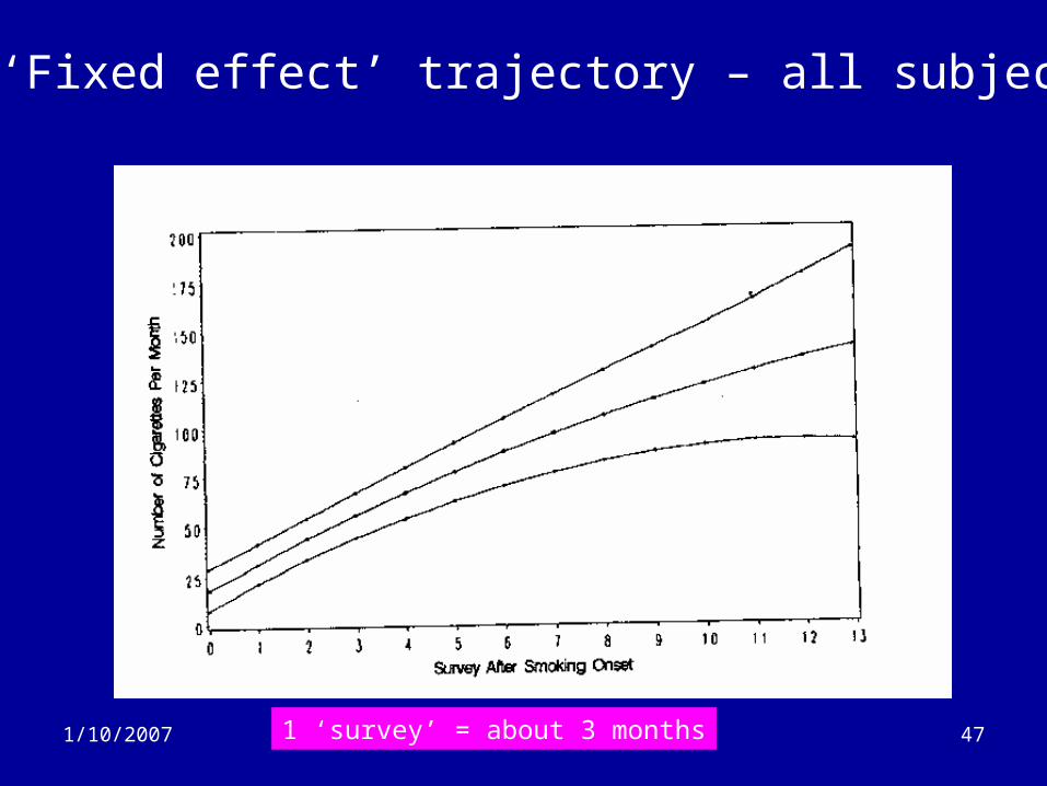
Application (2)

• Analysis– Step 1: multi-level model of change

• Used a quadratic trajectory model (time and time2)

– Mean smoking curve• 18 cigarettes per month in the first three months

after onset• Increased by 13.3 cigs/month every three months

– Strongly significant random effects• Evidence for strong heterogeneity in the

trajectories

1/10/2007 47

‘Fixed effect’ trajectory – all subjects

1 ‘survey’ = about 3 months

1/10/2007 48

Application (3)

• Step 2:– Explored a range of latent class models.– Best fit found with four latent groups– Graphs on next slide. Note that the

proportion of sample in each class varied greatly:

• Class 1: 73%• Class 2: 11%• Class 3: 11%• Class 4: 6%

1/10/2007 49

‘Latent class’ trajectories

Class 4

Class 3

Class 2

Class 1

Y-axis is reaches 750, not 200

1 ‘survey’ = about 3 months

1/10/2007 50

Application (4)

• Evidence of different characteristics among classes– Parents smoke: OR=2.2 (class 4)– Poor marks: OR > 4 (classes 3

& 4)– 50+% friends smoke: OR= 6 (class 3)

OR=12 (class 4)– Clear smoking rules: OR=0.3 (class 3)

OR=0.6 (class 4)

1/10/2007 51

Some things to consider:

• Spacing of time intervals – Repeated-measures ANOVA and MANOVA require that all

subjects be measured at same time intervals• smoking plots

– MANOVA weights all time intervals evenly (as if evenly spaced)

• Assumptions of the model– ALL strategies assume normally distributed outcome and

homogeneity of variances– But all strategies are robust against this assumption, especially if

data set is >30

• Missing Data– All traditional analyses assume that there is NO missing data

1/10/2007 52

Missing Data

• Very important to avoid missing data! • With missing data, changes in the mean over

time may just reflect drop-out pattern– You cannot compare time point 1 with 50 people to

time point 2 with 35 people!

• Prevention is best. Imputation is second choice.• One common ‘imputation’ method is:

– “last observation carried forward” strategy

• Other more complicated imputation strategies exist

1/10/2007 53

Wrap-up (1)

• The world is dynamic. Behaviour develops over time. Cross-sectional studies can be misleading and produce ‘bad’ policy.

• Having longitudinal data allows us to:– Study dynamic relationships– Study within subject changes– Study heterogeneity in trajectories

1/10/2007 54

Wrap-up (2)

• When designing research or evaluation studies, try to include follow-up components.– Before-after (2 data points) limit analysis

options– Follow-up studies should have 3 (or more)

measurement points.

1/10/2007 55

Warp-up (3)

• Over-all group trajectories can ‘hide’ important variation within sub-groups.– Not all teens who start smoking are heading to being

regular smokers.– Can provide insights to more efficiently target

intervention programmes.– Can provide insights into new interventions

approaches and targets.• Stage of change• At-risk behaviour differences

– Friends who smoke

1/10/2007 56

Acknowledgments

• Dr. J. O'Loughlin

• Dr. J. Singer

• Dr. J. Twisk

• Ms. K. Murphy

• Janice Potter

Documents

1/10/20071 APHEO: Longitudinal Data Analysis; Overview and Conceptual Ideas October 15, 2007 Dr. N. Birkett, Department of Epidemiology & Community Medicine,