Embed Size (px)
Citation preview

1111
Section X, Improvement
Techniques

2222
Will help you gain knowledge in:◦ Improving performance
characteristics◦ Reducing costs◦ Understand regression analysis◦ Understand relationships between
variables◦ Understand correlation◦ Understand how to optimize
processes
So you can:◦ Recognize opportunities◦ Understand terminology◦ Know when to get help
Objectives in Using DOE
X-2

3333
Let’s Start with an Example:
Plot a histogram and calculate the average and standard deviation
Data
18 16 30 29 28 21 17 41 8 1732 26 16 24 27 17 17 33 19 1831 27 23 38 33 14 13 26 11 2821 19 25 22 17 12 21 21 25 2623 20 22 19 21 14 45 15 24 34
Fuel Economy of 50 automobiles (in mpg)
Fuel Economy
0
2
4
6
8
10
12
14
16
0 to <6 6 to <12 12 to <18 18 to <24 24 to <30 30 to <36 36 to <42 42 to <48 48 to <54 54 to <=60mgp
Nu
mb
er
of
Ca
rs
7266.7
88.22
S
X
X-2

4444
Experimental design (a.k.a. DOE) is about discovering and quantifying the magnitude of cause and effect relationships.
We need DOE because intuition can be misleading.... but we’ll get to that in a minute.
Regression can be used to explain how we can model data experimentally.
What Might Explain the Variation?
METHOD
MOTHERNATUREMEASUREMENT
MANPOWER MACHINE
MATERIAL
X-2
5555
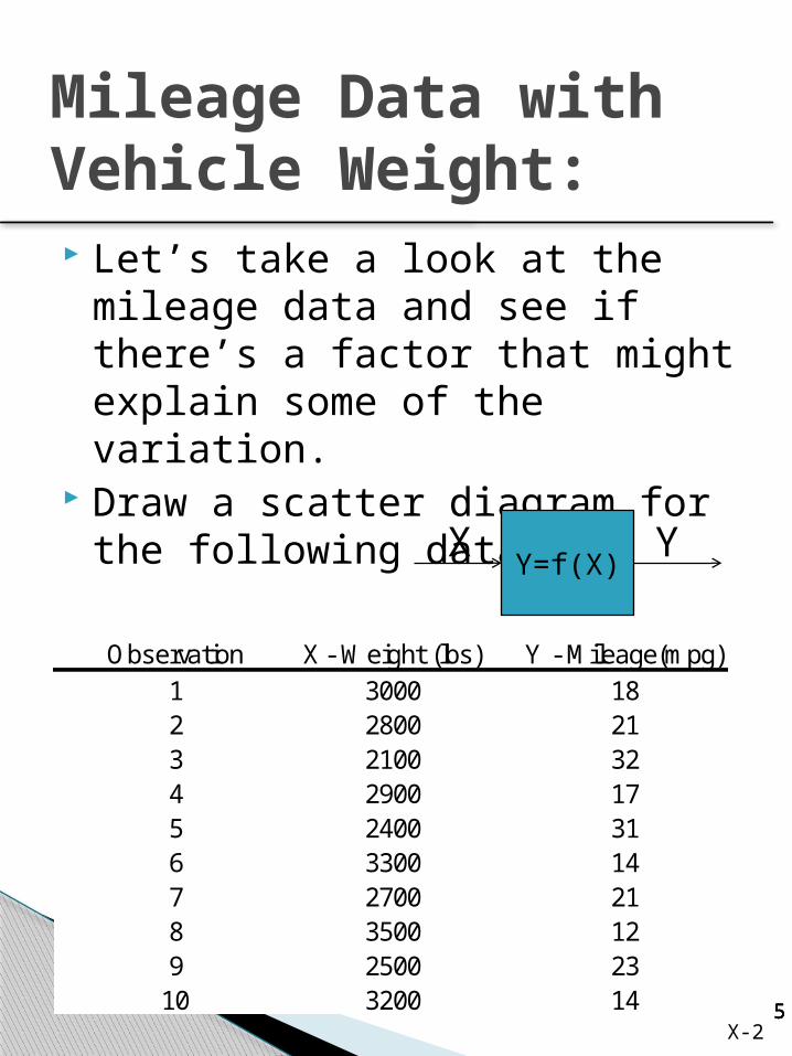
Let’s take a look at the mileage data and see if there’s a factor that might explain some of the variation.
Draw a scatter diagram for the following data:
Mileage Data with Vehicle Weight:
X - Weight (lbs) Y - Mileage(mpg)3000 182800 212100 322900 172400 313300 142700 213500 122500 233200 14
Observation1
10
6789
2345
Y=f(X)X Y
X-2

6666
If you draw a best fit line and figure out an equation for that line, you would have a ‘model’ that represents the data.
Regression Analysis
Scatter Chart (Weight vs mpg)
y = -0.0152x + 63.507
R2 = 0.9191
05
101520253035
1900 2400 2900 3400 3900
Weight
mp
g
Y=f(X)
X-2

7777
There are basically three ways to understand a process you are working on.
Classical 1FAT experiments ◦ One factor at a time (1FAT) focuses on one
variable at two or three levels and attempts to hold everything else constant (which is impossible to do in a complicated process).
Mathematical model◦ Express the system with a mathematical
equation. DOE
◦ When properly constructed, it can focus on a wide range of key input factors and will determine the optimum levels of each of the factors.
Each have their advantages and disadvantages. We’ll talk about each.
Understanding a System
X-2

8888
Let’s consider how two known (based on years of experience) factors affect gas mileage, tire size (T) and fuel type (F).
1FAT Example
Fuel Type Tire size
F1 T1
F2 T2
Y=f(X)
T(1,2)Y
F(1,2)
X-2
9999
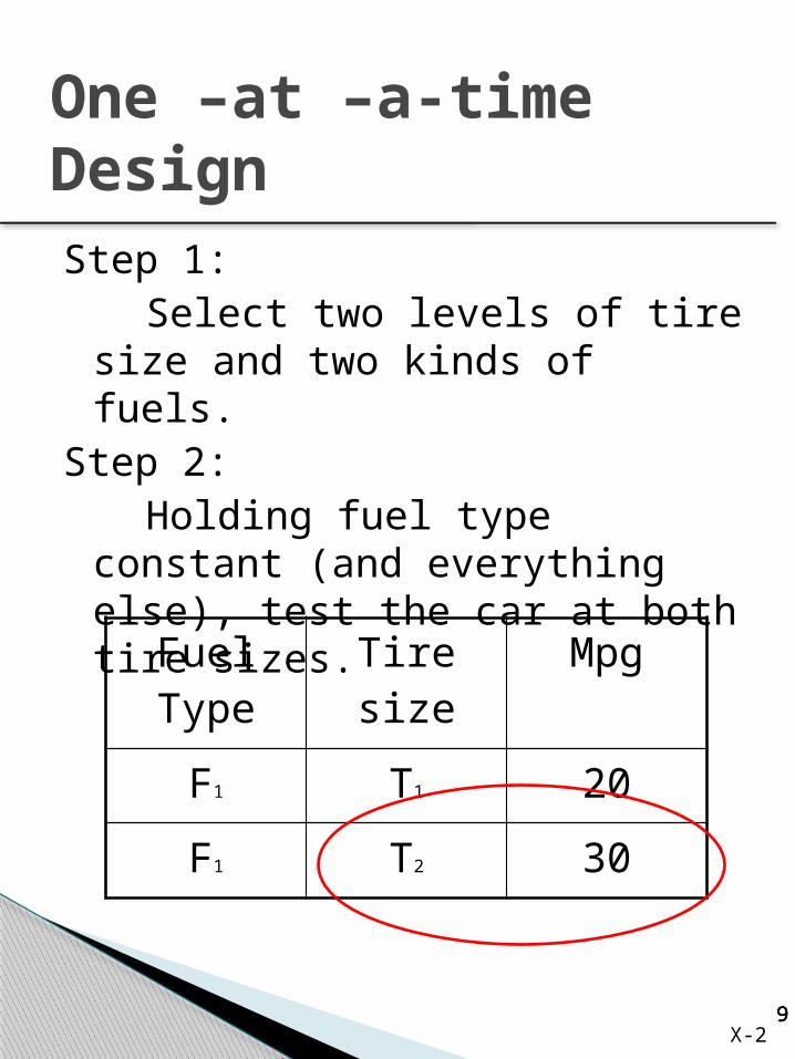
Step 1:Select two levels of tire
size and two kinds of fuels.Step 2:
Holding fuel type constant (and everything else), test the car at both tire sizes.
One –at –a-time Design
Fuel Type
Tire size Mpg
F1 T1 20
F1 T2 30
X-2

10101010
Since we want to maximize mpg the more desirable response happened with T2
Step 3: Holding tire size at T2, test the car at both fuel types.
One –at –a-time Design
Fuel Type
Tire size Mpg
F1 T2 30
F2 T2 40
X-2

11111111
Looks like the ideal setting is F2 and T2 at 40mpg.
This is a common experimental method.
One –at –a-time Design
Fuel Type
Tire size Mpg
F1 T2 30
F2 T2 40
What about the possible interaction effect of tire size and fuel type. F2T1
X-2

12121212
Suppose that the untested combination F2T1 would produce the results below.
There is a different slope so there appears to be an interaction. A more appropriate design would be to test all four combinations.
One –at –a-time Design
0
10
20
30
40
50
60
70
T1 T2
Tire Size
mpg
F2
F1
X-2
13131313
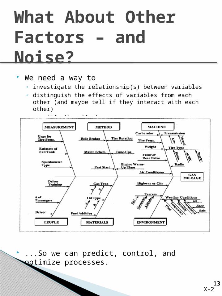
We need a way to ◦ investigate the relationship(s) between variables◦ distinguish the effects of variables from each other (and
maybe tell if they interact with each other)◦ quantify the effects...
...So we can predict, control, and optimize processes.
What About Other Factors – and Noise?
X-2

14141414
The Other Two Possibilities
We can see some problems with 1FAT. Now let’s go back and talk about the statapult.
We can do a mathematical model or we could do a DOE.
DOE will build a ‘model’ - a mathematical representation of the behavior of measurements.
or…
You could build a “mathematical model” without DOE and it might look something like...
X-2

15151515
A Mechanistic Model for the Statapult
X-2
16161616
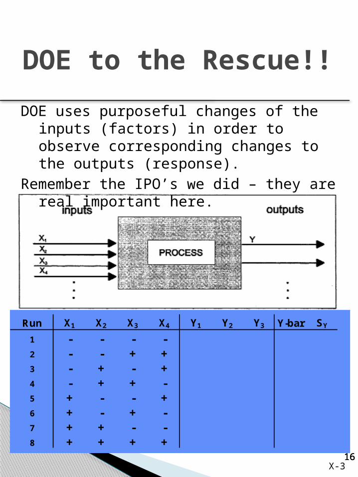
DOE to the Rescue!!
Run X1 X2 X3 X4 Y1 Y2 Y3 Y-bar SY
1 - - - -2 - - + +3 - + - +4 - + + -5 + - - +6 + - + -7 + + - -8 + + + +
DOE uses purposeful changes of the inputs (factors) in order to observe corresponding changes to the outputs (response).
Remember the IPO’s we did – they are real important here.
X-3

17171717
Set objectives (Charter)◦ Comparative
Determine what factor is significant◦ Screening
Determine what factors will be studied◦ Model – response surface method
Determine interactions and optimize Select process variables (C&E) and
levels you will test at Select an experimental design Execute the design CONFIRM the model!! Check that
the data are consistent with the experimental assumptions
Analyze and interpret the results Use/present the results
Planning - DOE Steps
X-4

18181818
Planning - Charter
X-8

19191919
Planning - Charter
http://jimakers.com/downloads/DOE_Setup.docxX-8

20202020
To ‘design’ an experiment, means to pick the points that you’ll use for a scatter diagram.
See DOE terms X-9 through X-15
The Basics
Run A B
1 - -2 - +3 + -4 + +
In tabular form, it would look like:
High (+)
Low (-)
Fa
cto
r B
Se
ttin
gs
Factor A Settings High (+)Low (-)
(-,+)
(+,-)
(+,+)
(-,-)
YA
B
X1
X2
X-9

21212121
A full factorial is an experimental design which contains all levels of all factors. No possible treatments are omitted. ◦ The preferred (ultimate) design◦ Best for modeling
A fractional factorial is a balanced experimental design which contains fewer than all combinations of all levels of all factors.◦ The preferred design when a full
factorial cannot be performed due to lack of resources
◦ Okay for some modeling ◦ Good for screening
Full vs.Fractional Factorial
X-16

22222222
Full factorial◦ 2 level◦ 3 factors◦ 8 runs◦ Balanced
(orthogonal)
Fractional factorial◦ 2 level◦ 3 factors◦ 4 runs - Half
fraction◦ Balanced
(orthogonal)
2 Level Designs
runs 823
runs 42 13
X-16

23232323
Res
pons
e - Y
Factor ALow High
Average Y when A was set ‘high’
Average Y when A was set ‘low’
The difference in the average Y when A was ‘high’ from the average Y when A was ‘low’ is the ‘factor effect’
The differences are calculated for every factor in the experiment
Measuring An “Effect”
X-16

24242424
When the effect of one factor changes due to the effect of another factor, the two factors are said to ‘interact.’
more than two factors can interact at the same time, but it is thought to be rare outside of chemical reactions.
Res
pons
e -
Y
Factor ALow High
B = High
B = Low
Slight
Res
pons
e -
Y
Factor ALow High
B = High B = Low
Strong
Looking For Interactions
Res
pons
e -
Y
Factor ALow High
B = High
B = LowNone
X-16

25252525
Using the statapult, we will experiment with some factors to “model” the process.
We will perform a confirmation run to determine if the model will help us predict the proper settings required to achieve a desired output.
Let’s Try This Out!
What design should we use?
YAB
X1
X2
CD
X3X4
Y=f(X1, X2, X3, X4)
X-17

26262626
Too much variation in the response
Measurement error Poor experimental discipline Aliases (confounded) effects Inadequate model Something changed
- And: -
Reasons Why a Model Might Not Confirm:
There may not be a true cause-and-effect relationship.
X-17

27272727
Remember?
X-17

28282828
Factor A B C D Response #1
Row #A -
B -
C -
D - Y1 Y2 Y3
1 -1 -1 -1 -1
2 -1 -1 -1 1
3 -1 -1 1 -1
4 -1 -1 1 1
5 -1 1 -1 -1
6 -1 1 -1 1
7 -1 1 1 -1
8 -1 1 1 1
9 1 -1 -1 -1
10 1 -1 -1 1
11 1 -1 1 -1
12 1 -1 1 1
13 1 1 -1 -1
14 1 1 -1 1
15 1 1 1 -1
16 1 1 1 1
Experiment Factorial Full
run 1624
X-17
Confirmation runs

29292929
Example Pages - Data
X-17

30303030
Marginal Means Plot
X-17

31313131
Regression Table
X-17

32323232
Prediction and Confirmation
X-17

33333333
Full factorial◦ 3 level◦ 3 factors◦ 27 runs◦ Balanced
(orthogonal)◦ Used when it is expected the
response in non-linear
3 Level Designs
runs 2733
X-18

34343434
Useful to see how factors effect the response and to determine what other settings provide the same response
2D Contour Plot
X-30

35353535
Helpful in reaching the optimal result
3D Response Surface Plot
X-30