Embed Size (px)
Citation preview

11.2 Comparing Distributions of a Categorical Variable Example – Does Background Music Influence What Customers Buy? Comparing conditional distributions Market researchers suspect that background music may affect the mood and buying behavior of customers. One study in a supermarket compared three randomly assigned treatments: no music, French accordion music, and Italian string music. Under each condition, the researchers recorded the numbers of bottles of French, Italian, and other wine purchased. Here is a table that summarizes the data: (a) Calculate the conditional distribution (in proportions) of the type of wine sold for each treatment. (b) Make an appropriate graph for comparing the conditional distributions in part (a).

(c) Are the distributions of wine purchases under the three music treatments similar or different? Give appropriate evidence from parts (a) and (b) to support your answer. In the example, we summarized the observed relationship between the type of music being played and the type of wine bought. The researchers expected that music would influence sales, so music type is the explanatory variable and the type of wine bought is the response variable. In general, the clearest way to describe this relationship is to compare the conditional distributions of the response variable for each value of the explanatory variable. That’s why we compared the conditional distributions of wine purchases for each type of music played.

CHECK YOUR UNDERSTANDING The Pennsylvania State University has its main campus in the town of State College and more than 20 smaller “commonwealth campuses” around the state. The Penn State Division of Student Affairs polled separate random samples of undergraduates from the main campus and commonwealth campuses about their use of online social networking. Facebook was the most popular site, with more than 80% of students having an account. Here is a comparison of Facebook use by undergraduates at the main campus and commonwealth campuses who have a Facebook account:
1. Calculate the conditional distribution (in proportions) of Facebook use for each campus setting. 2. Why is it important to compare proportions rather than counts in Question 1? 3. Make a bar graph that compares the two conditional distributions. What are the most important differences in Facebook use between the two campus settings?

The Problem of Multiple Comparisons The null hypothesis in the music and wine example is: H0: There is no difference in the distributions of wine purchases at this store when no music, French accordion music, or Italian string music is played. If the null hypothesis is true, the observed differences in the distributions of wine purchases for the three groups are due to the chance involved in the random assignment of treatments. The alternative hypothesis says that there is a difference but does not specify the nature of that difference: Ha: There is a difference in the distributions of wine purchases at this store when no music, French accordion music, or Italian string music is played. Any difference among the three actual distributions of wine purchases when no music, French accordion music, or Italian string music is played means that the null hypothesis is false and the alternative hypothesis is true. The alternative hypothesis is not one-‐sided or two-‐sided. We might call it “many-‐sided” because it allows any kind of difference. With only the methods we already know, we might start by comparing the proportions of French wine purchases when no music and French accordion music are played. We could similarly compare other pairs of proportions, ending up with many tests and many P-‐values. This is a bad idea. The P-‐values belong to each test separately, not to the collection of all the tests together. Think of the distinction between the probability that a virtual basketball player makes a free throw and the probability that she makes all her free throws in a game. When we do many individual tests or construct many confidence intervals, the individual P-‐values and confidence levels don’t tell us how confident we can be in all the inferences taken together. Because of this, it’s cheating to pick out one large difference from the two-‐way table and then perform a significance test as if it were the only comparison we had in mind. For example, the proportions of French wine bought under the no music and French accordion music treatments are 30/84 = 0.357 and 39/75 = 0.520, respectively. A two-‐sample z test shows that the difference between the proportions is statistically significant(z = 2.06, P = 0.039) if we make just this one comparison. But we could also pick a comparison that is not significant. For example, the proportions of Italian wine purchased for the no music and Italian string music treatment are 11/84 = 0.131 and 19/84 = 0.226, respectively. These two proportions do not differ significantly (z = 1.61, P = 0.107). Individual comparisons can’t tell us whether the three distributions of the categorical variable (in this case, wine bought) are significantly different.

The problem of how to do many comparisons at once with an overall measure of confidence in all our conclusions is common in statistics. This is the problem of multiple comparisons. Multiple comparisons Statistical methods for dealing with multiple comparisons usually have two parts:
1. An overall test to see if there is good evidence of any differences among the parameters that we want to compare.
2. A detailed follow-‐up analysis to decide which of the parameters differ and to estimate how large the
differences are. The overall test uses the familiar chi-‐square statistic and distributions. But in this new setting the test will be used to compare the distribution of a categorical variable for several populations or treatments. The follow-‐up analysis can be quite elaborate. We will concentrate on the overall test and use data analysis to describe the nature of the differences.

11.2.2 Expected Counts and the Chi-‐Square Statistic To perform a test of
• H0: There is no difference in the distribution of a categorical variable for several populations or treatments.
• Ha: There is a difference in the distribution of a categorical variable for several populations or treatments.
we compare the observed counts in a two-‐way table with the counts we would expect if H0were true. Finding the expected counts is not that difficult, as the following example illustrates. Example – Does Background Music Influence What Customers Buy? Computing expected counts The null hypothesis in the wine and music experiment is that there’s no difference in the distribution of wine purchases in the store when no music, French accordion music, or Italian string music is played. To find the expected counts, we start by assuming that H0 is true. We can see from the two-‐way table that 99 of the 243 bottles of wine bought during the study were French wines. If the specific type of music that’s playing has no effect on wine purchases, the proportion of French wine sold under each music condition should be 99/243 = 0.407. For instance, there were 84 bottles of wine bought when no music was playing. We would expect of those bottles to be French wine, on average. The expected counts of French wine bought under the other two music conditions can be found in a similar way:
We repeat the process to find the expected counts for the other two types of wine. The overall proportion of Italian wine bought during the study was 31/243 = 0.128. So the expected counts of Italian wine bought under each treatment are

The overall proportion of Other wine bought during the experiment was 113/243 = 0.465.So the expected counts of Other wine bought for each treatment are
The following table summarizes the expected counts for all three treatments. Note that the values for no music and Italian music are the same because 84 bottles of wine were bought under each condition. Although any count of bottles of wine sold must be a whole number, an expected count need not be. The expected count gives the average number of bottles sold if H0 is true and the random assignment process is repeated many times.
We can check our work by adding the expected counts to obtain the row and column totals, as in the table. These should be the same as those in the table of observed counts except for small roundoff errors, such as 75.01 rather than 75 for the total number of bottles of French wine sold.
Let’s take a look at the two-way table from the wine and music study one more time. In the example, we found the expected count of French wine bought when no music was playing as follows:
We marked the three numbers used in this calculation in the table. These values are the row total for French wine bought, the column total for wine purchased when no music was playing, and the table total of wine bought during the experiment. We can rewrite the original calculation as This suggests a more general formula for the expected count in any cell of a two-way table:


11.2.3 The Chi-‐Square Test for Homogeneity Earlier, we used a chi-‐square goodness-‐of-‐fit test to test a hypothesized model for the distribution of a categorical variable. Our P-‐values came from a chi-‐square distribution with df = the number of categories − 1. When the Random, Large Sample Size, and Independent conditions are met, the χ2 statistic calculated from a two-‐way table can be used to perform a test of H0: There is no difference in the distribution of a categorical variable for several populations or treatments. P-‐values for this test come from a chi-‐square distribution with df = (number of rows − 1)(number of columns − 1). This test is also known as a chi-‐square test for homogeneity of proportions. We prefer the simpler name.

Example – Does Background Music Influence What Customers Buy? P-‐value and conclusion Earlier, we started a significance test of: H0: There is no difference in the distributions of wine purchases at this store when no music, French accordion music, or Italian string music is played. Ha: There is a difference in the distributions of wine purchases at this store when no music, French accordion music, or Italian string music is played.
(a) Calculate the chi-‐square test statistic and the P-‐value using your calculator’s χ2 cdf command. Show your work. (b) Interpret the P-‐value from the calculator in context. (c) What conclusion would you draw? Justify your answer.

CHECK YOUR UNDERSTANDING The Pennsylvania State University has its main campus in the town of State College and more than 20 smaller “commonwealth campuses” around the state. The Penn State Division of Student Affairs polled separate random samples of undergraduates from the main campus and commonwealth campuses about their use of online social networking. Facebook was the most popular site, with more than 80% of students having an account. Here is a comparison of Facebook use by undergraduates at the main campus and commonwealth campuses who have a Facebook account:
Do these data provide convincing evidence of a difference in the distributions of Facebook use among students in the two campus settings? 1. State appropriate null and alternative hypotheses for a significance test to help answer this question. 2. Calculate the expected counts. Show your work. 3. Calculate the chi-square statistic. Show your work.

4. Use your calculator’s χ2 cdfcommand to find the p-value. 5. Interpret the P-value from the calculator in context. 6. What conclusion would you draw? Justify your answer. Learn Chi-‐square tests for two-‐way tables on the calculator

Example – Are Cell-‐Only Telephone Users Different? The chi-‐square test for homogeneity Random digit dialing telephone surveys used to exclude cell phone numbers. If the opinions of people who have only cell phones differ from those of people who have landline service, the poll results may not represent the entire adult population. The Pew Research Center interviewed separate random samples of cell-‐only and landline telephone users who were less than 30 years old. Here’s what the Pew survey found about how these people describe their political party affiliation: (a) Construct an appropriate graph to compare the distributions of political party affiliation for cell-‐only and landline phone users. Because the sample sizes are different, we should compare the proportions of individuals in each political affiliation category in the two samples. The table shows the conditional distributions of political party affiliation for cell-‐only and landline phone users. We made a segmented bar graph to compare these two distributions. (b) Do these data provide convincing evidence that the distribution of party affiliation differs in the cell-‐only and landline user populations? Carry out a significance test at the α = 0.05 level. STATE: We want to perform a test of H0: There is no difference in the distribution of party affiliation in the cell-‐only and landline populations. Ha: There is a difference in the distribution of party affiliation in the cell-‐only and landline populations. at the α = 0.05 level.

PLAN: If conditions are met, we should use a chi-‐square test for homogeneity
• Random The data came from separate random samples of 96 cell-‐only and 104 landline users. • Large Sample Size We followed the steps in the technology Corner to get the expected counts. All the
expected counts are at least 5. • Independent Researchers took independent samples of cell-‐only and landline phone users. Sampling
without replacement was used, so there need to be at least 10(96) = 960 cell-‐only users under age 30 and at least 10(104) = 1040 landline users under age 30. this is safe to assume.
Do: A chi-‐square test on the calculator gave
• Test statistic
P-‐value Using df = (number of rows − 1)(number of columns − 1) = (3 − 1)(2 − 1)= 2, the P-‐value is 0.20. CONCLUDE: Because our P-‐value, 0.20, is greater than α = 0.05, we fail to reject H0.There is not enough evidence to conclude that the distribution of party affiliation differs in the cell-‐only and landline user populations.
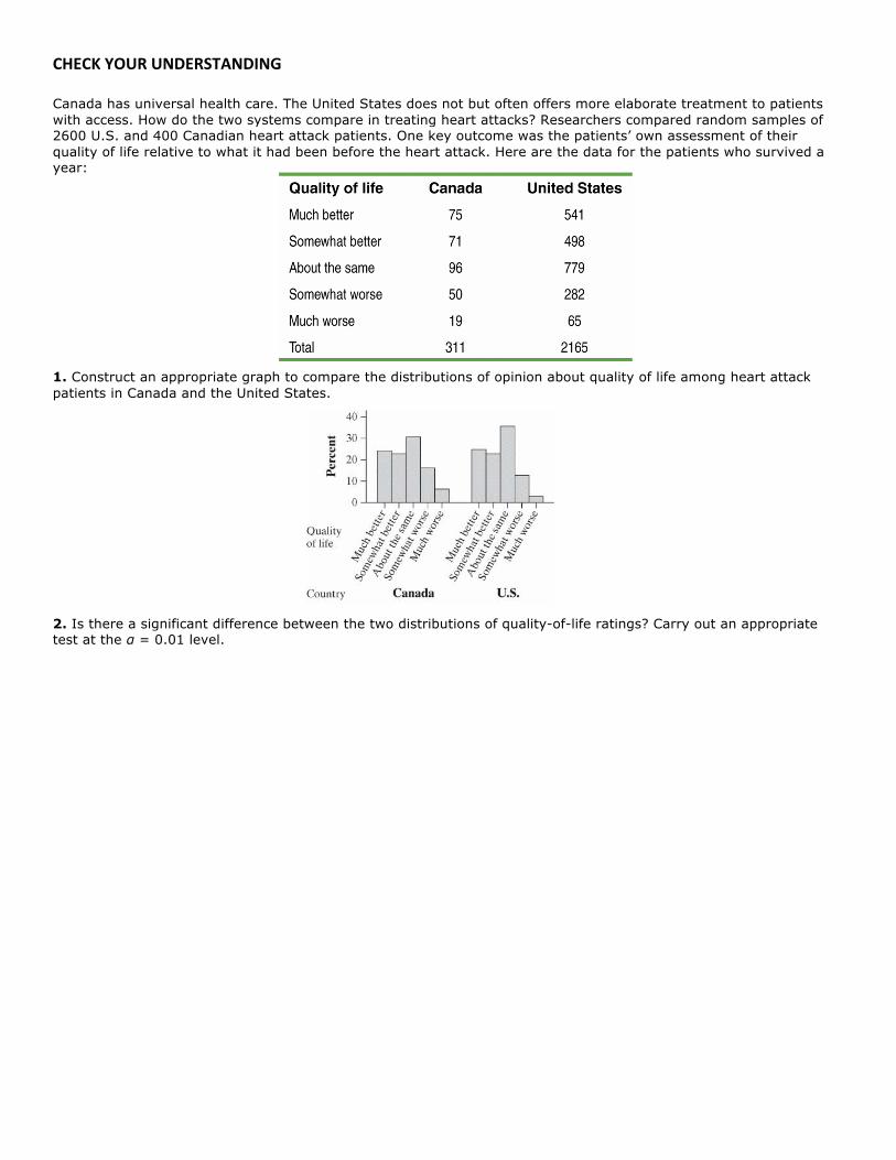
CHECK YOUR UNDERSTANDING Canada has universal health care. The United States does not but often offers more elaborate treatment to patients with access. How do the two systems compare in treating heart attacks? Researchers compared random samples of 2600 U.S. and 400 Canadian heart attack patients. One key outcome was the patients’ own assessment of their quality of life relative to what it had been before the heart attack. Here are the data for the patients who survived a year: 1. Construct an appropriate graph to compare the distributions of opinion about quality of life among heart attack patients in Canada and the United States. 2. Is there a significant difference between the two distributions of quality-of-life ratings? Carry out an appropriate test at the α = 0.01 level.

11.2.4 Follow-‐up Analysis The chi-‐square test for homogeneity allows us to compare the distribution of a categorical variable for any number of populations or treatments. If the test allows us to reject the null hypothesis of no difference, we then want to do a follow-‐up analysis that examines the differences in detail. Start by examining which cells in the two-‐way table show large deviations between the observed and expected counts. Then look at the individual components to see which terms contribute most to the chi-‐square statistic.

11.2.5 Comparing Several Proportions Many studies involve comparing the proportion of successes for each of several populations or treatments. The two-‐sample z test from Chapter 10 allows us to test the null hypothesis H0: p1 = p2, where p1 and p2 are the actual proportions of successes for the two populations or treatments. The chi-‐square test for homogeneity allows us to testH0: p1 = p2 = ·∙·∙·∙ = pk. This null hypothesis says that there is no difference in the proportions of successes for the k populations or treatments. The alternative hypothesis is Ha: at least two of the pi’s are different. Many students incorrectly state Ha as “all the proportions are different.” Think about it this way: the opposite of “all the proportions are equal” is “some of the proportions are not equal.” Example – Cocaine Addiction Is Hard to Break Comparing proportions of successes Cocaine addicts need cocaine to feel any pleasure, so perhaps giving them an antidepressant drug will help. A three-‐year study with 72 chronic cocaine users compared an antidepressant drug called desipramine with lithium (a standard drug to treat cocaine addiction) and a placebo. One-‐third of the subjects were randomly assigned to receive each treatment. Here are the results: (a) Make a graph to compare the rates of cocaine relapse for the three treatments. Describe what you see. The distributions of cocaine relapse outcomes for the three treatment groups are The bar graph below compares the proportion of subjects who relapsed in the three groups. A much smaller proportion of subjects relapsed in the desipramine group than in either the lithium or placebo groups.

STATE: We want to perform a test of
where pi = the actual proportion of chronic cocaine users like the ones in this experiment who would relapse under treatment i. We’ll use α = 0.01 as instructed. PLAN: If conditions are met, we should carry out a chi-‐square test for homogeneity.
• Random The subjects were randomly assigned to the three treatment groups. • Large Sample Size We can use our familiar formula to find the expected counts from the two-‐way table
assuming that H0 is true:
• The row total is 24 for all three groups, and the column totals are Yes = 48 and No = 24. So the
expected count of subjects who relapse under each treatment is The expected count
of subjects who don’t relapse under each treatment is . All the expected counts are at least 5, so this condition is met.
• Independent The random assignment helps create three independent groups. if the experiment is
conducted properly, then knowing one subject’s relapse status should give us no information about another subject’s outcome. So individual observations are independent.
DO: We used the calculator’s chi-‐square test to do the calculations.
P-‐value With df = (number of rows − 1)(number of columns − 1) = (3 − 1)(2 − 1) = 2, the calculator gives P = 0.0052. CONCLUDE: Because the P-‐value, 0.0052, is less than α = 0.01, we have sufficient evidence to reject H0 and conclude that the true relapse rates for the three treatments are not all the same.

CHECK YOUR UNDERSTANDING Sample surveys on sensitive issues can give different results depending on how the question is asked. A University of Wisconsin study randomly divided 2400 respondents into three groups. All participants were asked if they had ever used cocaine. One group of 800 was interviewed by phone; 21% said they had used cocaine. Another 800 people were asked the question in a one-on-one personal interview; 25% said “Yes.” The remaining 800 were allowed to make an anonymous written response; 28% said “Yes.” 1. Was this an experiment or an observational study? Justify your answer. 2. Make a two-way table of responses about cocaine use by how the survey was administered. 3. Are the differences between the three groups statistically significant? Give appropriate evidence to support your answer.

11.2.6 Relationships between Two Categorical Variables Two-‐way tables can arise in several ways. The music and wine experiment compared three music treatments using independent groups of observations. The phone use and political party affiliation observational study compared independent random samples from the cell-‐only and landline user populations. In both cases, we are comparing the distributions of a categorical variable in several populations or treatments. We use the chi-‐square test for homogeneity to perform inference in such settings. Another common situation that leads to a two-‐way table is when a single random sample of individuals is chosen from a single population and then classified according to two categorical variables. In that case, our goal is to analyze the relationship between the variables. The next example describes a study of this type. Example – Do Angry People Have More Heart Disease Relationships between two categorical variables A study followed a random sample of 8474 people with normal blood pressure for about four years. All the individuals were free of heart disease at the beginning of the study. Each person took the Spielberger Trait Anger Scale test, which measures how prone a person is to sudden anger. Researchers also recorded whether each individual developed coronary heart disease (CHD). This includes people who had heart attacks and those who needed medical treatment for heart disease. Here is a two-‐way table that summarizes the data: (a) Calculate appropriate conditional distributions (in proportions) to describe the relationship between anger level and CHD status. Since we’re interested in whether angrier people tend to get heart disease more often, we can compare the percents of people who did and did not get heart disease in each of the three anger categories: (b) Make a well-‐labeled graph that compares the conditional distributions in part (a). The bar graph below shows the percent of people in each of the three anger categories who developed CHD.

(c) Write a few sentences describing the relationship between the two variables. There is a clear trend: as the anger score increases, so does the percent who suffer heart disease. A much higher percent of people in the high anger category developed CHD (4.27%) than in the moderate (2.33%) and low (1.70%) anger categories. Anger rating on the Spielberger scale is a categorical variable that takes three possible values: low, medium, and high. Whether or not someone gets heart disease is also a categorical variable. The two-way table in the example shows the relationship between anger rating and heart disease for a random sample of 8474 people. Do these data provide convincing evidence of an association between the variables in the larger population? To answer that question, we work with a new significance test.

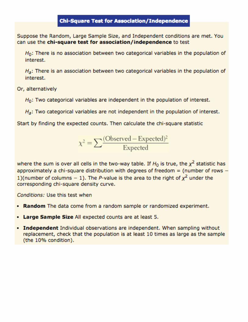
11.2.7 The Chi-‐Square Test for Association/Independence We often gather data from a random sample and arrange them in a two-‐way table to see if two categorical variables are associated. The sample data are easy to investigate: turn them into percents and look for a relationship between the variables. Is the association in the sample evidence of an association between these variables in the entire population? Or could the sample association easily arise just from the luck of random sampling? This is a question for a significance test. Our null hypothesis is that there is no association between the two categorical variables. The alternative hypothesis is that there is an association between the variables. For the observational study of anger level and coronary heart disease, we want to test the hypotheses: H0: There is no association between anger level and heart disease in the population of people with normal blood pressure. Ha: There is an association between anger level and heart disease in the population of people with normal blood pressure. No association between two variables means that the values of one variable do not tend to occur in common with values of the other. That is, the variables are independent. An equivalent way to state the hypotheses is therefore H0: Anger and heart disease are independent in the population of people with normal blood pressure. Ha: Anger and heart disease are not independent in the population of people with normal blood pressure. As with the two previous types of chi-‐square tests, we begin by comparing the observed counts in a two-‐way table with the expected counts if H0 is true.

Example – Do Angry People Have More Heart Disease? Finding expected counts The null hypothesis is that there is no association between anger level and heart disease in the population of interest. If we assume that H0 is true, then anger level and heart disease are independent. We can find the expected cell counts in the two-‐way table using the definition of independent events from Chapter 5: P(a | B) = P(a). Let’s start by considering the events “CHD” and “low anger.” We see from the two-‐way table that 190 of the 8474 people in the study had CHD. If we imagine choosing one of these people at random, P(CHD) = 190/8474. Because anger level and heart disease are independent, knowing that the selected individual is low anger gives us no additional information about the chance that this person has heart disease. That is, P(CHD | low anger) = P(CHD) = 190/8474. Of the 3110 low-‐anger people in the study, we’d expect to get CHD. We could also write this as You can see that the general formula we developed earlier for a test for homogeneity applies in this situation also: We find the expected counts for all the cells in the two-‐way table in a similar way.

Example – Do Angry People Have More Heart Disease Chi-‐square test for association/independence Here is the complete table of observed and expected counts for the CHD and anger study side by side: Do the data provide convincing evidence of an association between anger level and heart disease in the population of interest? Carry out an appropriate test to help answer this question. State: We want to perform a test of
• H0: there is no association between anger level and heart disease in the population of people with normal blood pressure.
• Ha: there is an association between anger level and heart disease in the population of people with normal blood pressure.
Since no significance level was stated, we’ll use α = 0.05. PLAN: If conditions are met, we should carry out a chi-‐square test of association/independence.
• Random The data came from a random sample of 8474 people with normal blood pressure. • Large Sample Size all the expected counts are at least 5, so this condition is met. • Independent Because we are sampling without replacement, we need to check that the total number
of people in the population with normal blood pressure is at least 10(8474) = 84,740. this seems reasonable to assume. Thus, knowing the values of both variables for one person in the study gives us no meaningful information about the values of the variables for another person. So individual observations are independent.
Do: We perform calculations assuming H0 is true.
P-‐value The two-‐way table of anger level versus heart disease has 2 rows and 3 columns. We will use the chi-‐square distribution with df = (2 − 1)(3 − 1) = 2 to find the P-‐value. The command χ2 cdf(16.077,1000,2) gives 0.00032. CONCLUDE: Because the P-‐value is clearly less than α = 0.05, we have sufficient evidence to reject H0 and conclude that anger level and heart disease are associated in the population of people with normal blood pressure.

CHECK YOUR UNDERSTANDING Many popular businesses are franchises—think of McDonald’s. The owner of a local franchise benefits from the brand recognition, national advertising, and detailed guidelines provided by the franchise chain. In return, he or she pays fees to the franchise firm and agrees to follow its policies. The relationship between the local owner and the franchise firm is spelled out in a detailed contract.
One clause that the contract may or may not contain is the entrepreneur’s right to an exclusive territory. This means that the new outlet will be the only representative of the franchise in a specified territory and will not have to compete with other outlets of the same chain. How does the presence of an exclusive-territory clause in the contract relate to the survival of the business?
A study designed to address this question collected data from a random sample of 170 new franchise firms. Two categorical variables were measured for each franchisor. First, the franchisor was classified as successful or not based on whether or not it was still offering franchises as of a certain date. Second, the contract each franchisor offered to franchisees was classified according to whether or not there was an exclusive-territory clause. Here are the count data, arranged in a two-way table:
Do these data provide convincing evidence of an association between an exclusive-territory clause and business survival? Carry out an appropriate test at the α = 0.01 level.