PA98 - 1 - 052

ABSTRACT

PROCEEDINGS, INDONESIAN PETROLEUM ASSOCIATION Twenty-Sixth Annual Convention, May 1998

WHERE IS M Y HOFUZONTAL WELL ? USE OF BOREHOLE SEISMIC WHERE VELOCJTIES VARY LATERALLY

Agus Muharam" Frank Musgmve"

Extended offset horizontal wells (out to a kilometer or more) are becoming common in field developments. In areas where overburden velocity varies laterally, it becomes difficult to know where the well is relative to the top of the reservoir away from the top reservoir penetration point. This is important to know for depth conversion and volumetrics and to know what part of the reservoir is sampled by the well to build a good simulation model for reservoir characterization.

We examine the use of the conventional offset VSP method but it can only image reflectors below the reservoirs in the well making receivers in the horizontal section only good for imaging the base reservoir. The top reservoir over the horizontal section could only be imaged by a very far offset source recorded by receivers in the vertical section giving raypaths with too much moveout, poor signal quality and little control on overburden velocity. Instead, we have applied a checkshot solution to the problem where we can use the seismic time and the checkshot time to estimate borehole location relative to the top reservoir and'the overburden velocity for depth conversion.

Examples from onshore North Sumatra illustrate the ideal and practical methods and the accuracy of our estimates. The marine applications are very accurate (2 20 feet in the estimate of well position relative to the top reservoir) due to more homogeneous near surface and the ability to easily locate the source directly over the receiver. The land applications are less accurate but still more accurate than no information (2 60 feet), due to more variable near

* Mobil Oil Indonesia, Inc.

surface statics, datuming velocities and the inability to easily locate the source over the receiver.

INTRODUCTION

There are many reasons stated for not acquiring borehole seismic data in development wells. They usually consider that enough velocity information is available in the field from wildcat and appraisal control, velocity surveys, and development well penetration points to make a reasonably accurate depth conversion. Extended offset horizontal wells have added a new complexity to the question that has made us consider the value of additional data from the development wells.

Mobil Oil Indonesia has operated the drilling of 20 highly deviated development wells in 1997 to develop four Peutu limestone fields in North Sumatra. Seven of these wells, in the SLS-A' & D fields, have offsets of approximately 2,625 feet. After drilling each well, we know the position of the whole well bore in depth but we only know the depth of the top of the reservoir where the well penetrates it. What we don't know is the depth to the top of the reservoir over the horizontal well bore. We only know that surface in time from the surface seismic. If this were an area of well behaved overburden velocity, it would be sufficient to depth convert the top reservoir surface with the velocity from the well penetration .points and the wildcat velocity surveys. Unfortunately, this area is an onshore area in the foothills of the Barisan Uplift topography. Both statics and laterally varying velocities are a problem. We would like to acquire borehole seismic data that allow us to better know the top reservoir surface in depth, the position of the horizontal well bore relative to it, and which layers in the reservoir have been sampled by the well bore (for

© IPA, 2006 - 26th Annual Convention Proceedings, 1998

118

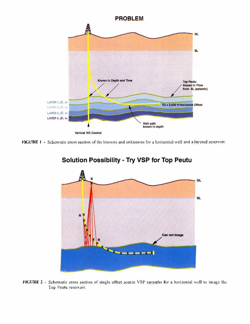
the simulator model). Figure 1 illustrates the time to depth problem for a general case.

SOLUTIONS

The first solution we tried to model was whether a VSP image of the Top reservoir (Top Peutu in this case) would answer our questions. Figure 2 is a model of the reflection points for a relatively near offset VSP. Reflections can only be imaged where the borehole is above the reservoir giving a very small image of an area that is already well known from the well penetration points in this case. The top re'servoir surface above the horizontal well bore cannot be imaged at this offset. We could move the source out farther away from the surface location of the well but the source would need to be approximately 2.5 km from the well (assumes highest receiver half way up well bore and reflection point at 2,625 feet offset). This poses several problems such as weak signal from long distance travel, energy arriving at high angle from vertical, and lack of control on velocity needed to migrate and depth convert the VSP data.

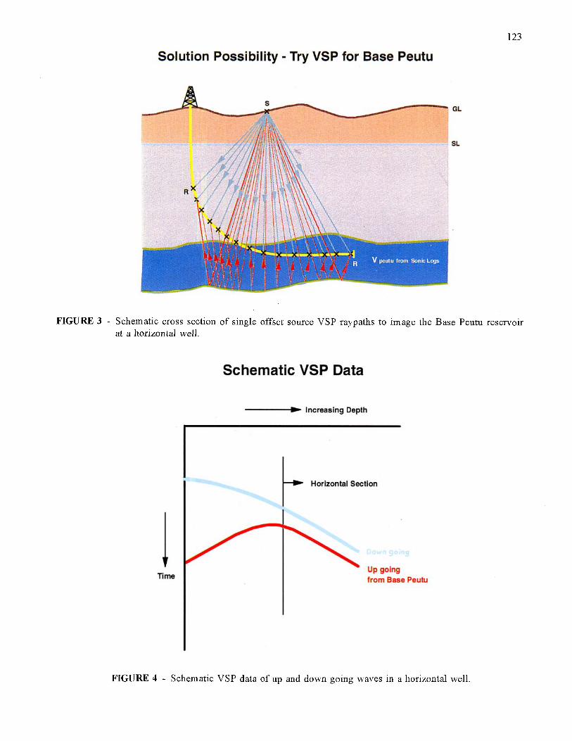
The second solution considered was a more reasonable offset VSP to image the base of the reservoir (Figure 3). The first constraint here is that there must be a good reflecting interface at the base *reservoir to image. Second, the reservoir thickness must be known. If there are reflectors at top and base reservoir, the thickness could be estimated by applying a reservoir interval velocity estimate (from vertical wildcat sonic or checkshot data). But the horizontal well is still a problem for VSP processing. The data would look like Figure 4. The up-going and down- going arrivals would only be dip separable for receivers in the non-horizontal portion of the well bore. Data from the horizontal section would show a small time lag between the parallel direct and reflected events. These events would be very difficult to separate by deconvolution since there is no slope difference. We did not try this method because of the obvious problems and because there is not always a good base reservoir reflector at SLS.

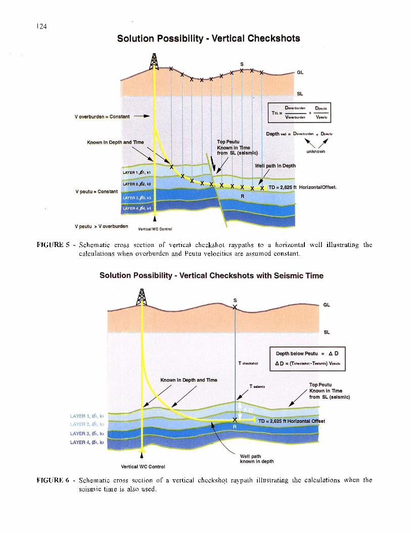
Next we examined the use of checkshot data. The simplest case is that of a sources vertically above receivers (Figure 5) . We measure total travel time and receiver depth only. Interval velocities of the overburden and the reservoir can not be measured or

derived from this data bedause the top reservoir is near horizontal and the well bore is near parallel with the top reservoir (Smidt, 1996). The depth to the top reservoir (Doverbllrden) and the depth of the well below the top reservoir (D,,,J can be derived from the two equations in Figure 5 (two equations, two unknowns) only if we assume constant velocities for VoverbnrdeI, and Vyeut1, and if the two velocities are substantially different. In the SLS case, the velocities are quite different between the overburden shale and the reservoir reefal limestone but the assumption of constant overburden velocity is not well founded. Statics and variable velocity in this thrusted overburden have made considerable error in our depth convcrsions and well prognoses of previous wells.

Where the overburden velocity is variable (the same places we generally need checkshot information), we must have another piece of information. Figure 6 shows a method that uses the seismic data time to the top reservoir with the checkshot data. The depth to the receiver in the borehole is known and the depth of the top reservoir surface is calculated by subtracting the delta D betwe& the receiver and the top reservoir surface. Delta D is calculated from the difference between the seismic time to top reservoir reflector and checkshot time to borehole receiver divided by the reservoir interval velocity (from sonic logs). The obvious requirements for this method are a good top reservoir reflector, known phase and polarity of seismic and checkshot data, and a method to correct both data sets to a common datum (knowledge of shallow velocity structure).

If there is not a good top reservoir reflector to use this method, the intcrprcter must revert to the previous method that doesn't use the seismic data (Figure 5 ) . When the seismic data is not used, calculated changes in the depth of the borehole below the top reservoir surface will have iarge error associated with them due to the unknown magnitude of variation in Voverburdeli but the method will still show large variations in the depth of the top reservoir over short distances (such as faults) where the checkshot recorded time should change sharply between receiver positions straddling the fault (assumes large velocity difference between overburden and reservoir as with carbonates overlain by shale). This could be particularly useful for reservoir characterization where the top reservoir surface is not well imaged by seismic.

119

OPERATIONAL CONSIDERATIONS

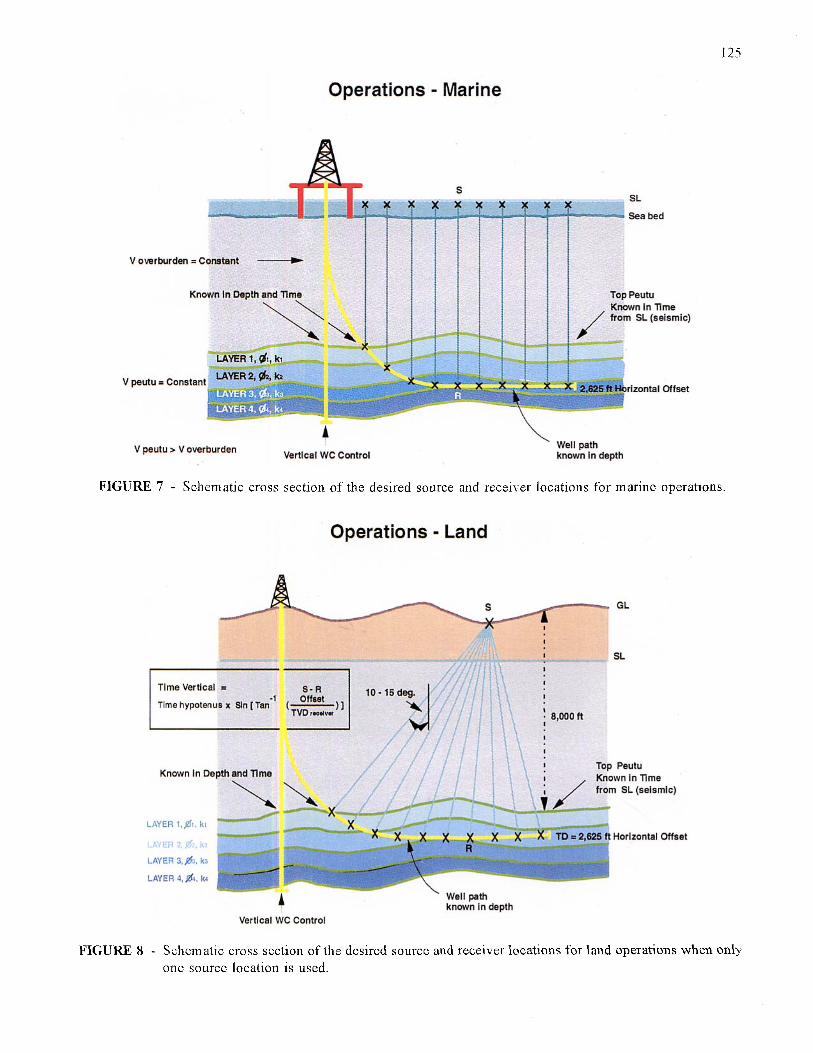
The marine case is optimal for doing checkshots over horizontal wells (Figure 7). Airguns can be placed directly over the receiver location (vertical travel path, direct comparison to seismic stack trace) and very close to the sea level datum (small correction from source position to datum). The land case usually presents more constraints. Topography, surface conditions , ,physical, cultural, and environmental obstacles often conspire to limit the possible source locations. If dynamite is used, shot holes must be drilled. If airguns are used, large pits must be excavated. At SLS, we were only able to use one airgun pit for each well. Due to the mountainous and forested nature of the area, we always attempted to dig the pit on or near to a road. We tried to find a location as close as possible to the well TD position to minimize the nonvertical ray path angle correction error and as far away from the well penetration and wildcat known control points as possible. The nonvertical angle correction increases as the receiver is moved away from the source position (Figure 8).

ACCURACY

The marine case has many less potential errors than the land case. In marine acquisition, there is no angle correction as the shot is vertically over the receiver. Both the seismic data and the checkshot data have the source airgun near the datum in the known velocity water layer. Therefore there should be no difference in statics or datum corrections. Measurement and calculation errors are all small including :

1. Seismic time error due to inaccurate migration velocity if top reservoir is not nearly flat,

2. Error in picking checkshot first break up to 2 ms = 13 feet,

3. Error in reservoir velocity 2 500 ft/sec = 6 feet, and

4. Only small error in picking seismic time if polarity and phase are known.

Therefore in the ideal case of marine data, known polarity and phase and nearly flat top reservoir locally, the depth estimate should be accurate within k 20 feet. Potentially the largest error is in not knowing

the seismic polarity and phase well enough. If it is picked '/4 wavelet off (90" out of phase) for a 20 Hz dominant frequency wavelet and 8,000 ft/sec velocity, an additional 50 feet error will be introduced. Wavelet processing, analysis of shallow gas 'anomalies, water bottom, and other events of known reflection coefficient should reduce the potential for this error to occur. Also, we can compare the checkshot data and seismic time picks at well penetration points where the top reservoir depth is known. A correction velocity can be calculated that moves the checkshot data from the gun elevation to the seismic datum and makes the seismic and checkshot times equal at the well penetrations. The most reasonable gun depth to datum correction velocity will result from the comparison when the correct wavelet polarity and phase are used for the seismic pick.

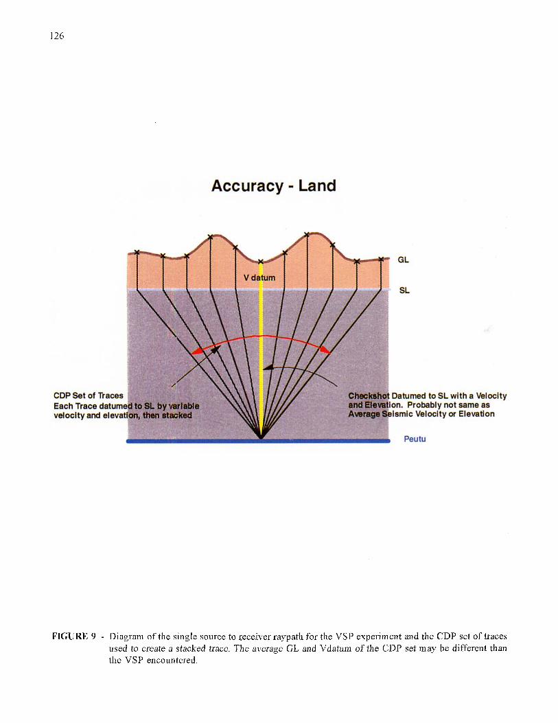
The land case has ail of the same errors as the marine case with the addition of statics and datuming errors and non vertical raypath corrections for some receiver positions (Figure 8). If we consider the receiver positions where the raypath is near vertical, only the statics and datuming will add error. Figure 9 illustrates the problem in equating the seismic and the checkshot experiments. The checkshot is a single raypath experiment where the time must be adjusted downward to the datum. The seismic trace is the result of stacking a CDP set of traces that have different elevations, correction velocities, and statics. We must use a correction velocity for the checkshot that makes the checkshot time best match that of the seismic data at reservoir penetration points. It will be an average of the correction velocities in the CDP set. The best way to derive a range of velocities is by making checkshots and seismic reflectors tie at area wildcat wells and deviated well penetration points. If the datum correction velocity can only be determined to within 1000 ft/sec, there will be an additional 2 44 feet error associated with the delta D depth for the SLS case. This is calculated where the datum is 200 feet and the velocity of the reservoir is 13,000 ft/sec. The seismic to checkshot time comparison will have a & 6.7ms one-way time error {(200ft/6,000ft/sec) - (200ft/5,000ft/sec)}. The dep,th error is k 44 feet if the middle datum correction velocity is used (.0067 x 13,000/2). If the reservoir is several hundred feet thick, this level of accuracy would be sufficient to add knowledge to the reservoir model and the volumetric calculations.

120

CASE HISTORY

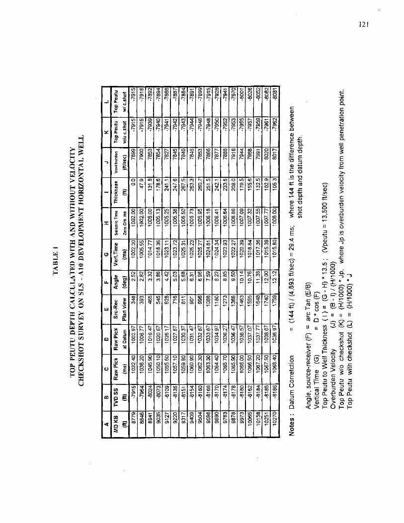
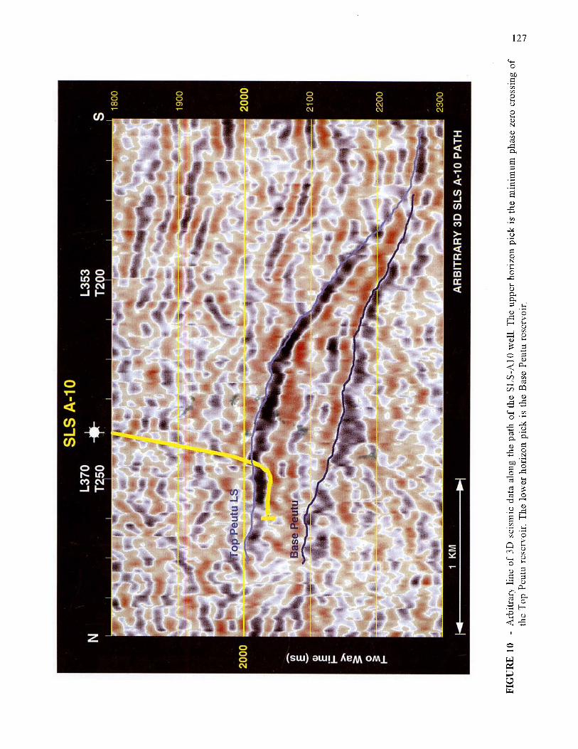
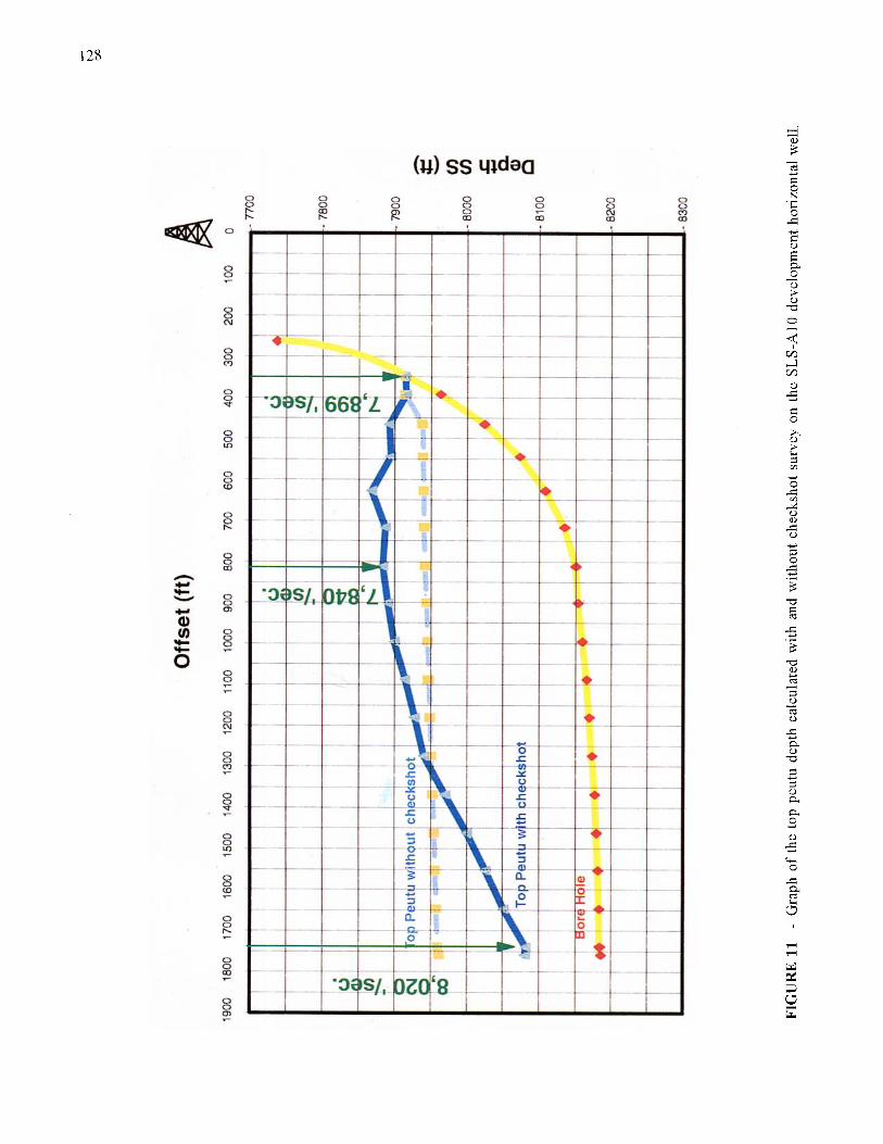
Checkshot data in some wells showed that the overburden velocity was not highly variable and that the data was not needed while others showed that the velocity was quite variable and that the data added value. The problem with this conclusion is that we would not know this unless we had the data. One of the wells that gave significant results was the SLS- A10 well onshore 'B' Block North Sumatra. The reflector at the top of the reef is a prominent peak on this 3D data set (black, Figure 10) and is easily interpreted over the well horizontal section and appears to be almost flat. If the seismic top reservoir surface had been depth converted with the velocity from the well penetration, it would be nearly flat (Figure 11). However, when the checkshot and seismic data are used to calculate the depth of the well bore below the top reservoir (delta D) and the velocity of the overburden (by the method outline in Figure 6, calculations Table 1) our depth estimates would have been over 100 feet off (compare columns K and L, Table 1 and graphically Figure 11). The velocity decreases over the middle well section raising the top reservoir in depth and then increases toward the well TD depressing the top reservoir in depth. Clearly, this information is valuable for depth conversion, volumetrics and creation of a simulation model.

We estimate that our top reservoir depths are accurate to within approximately 2 50 feet. The datum correction error has been minimized by using a velocity (4,893 ft/sec) which makes the seismic time (zero crossing, peak, minimum phase) and the checkshot time equal at the well penetration point. Physically, this is a very reasonable velocity for the shallow overburden and it matches well with the correction velocities calculated by a similar method in

the other wells of the field. Potentially the largest error in this example is the slant path correction since there was only one airgun pit. For locations away from the source location, the seismic data traveled sub-vertically whereas the checkshot data traveled a slant path sampling a different velocity field. A second VSP source at the other end of the borehole would minimize these possible errors. Our opinion is that the magnitudes of the velocity and depth changes are not highly accurate but that the trends in velocity and depth are real and meaningful.

CONCLUSIONS

VSP and checkshot methods have been examined for application to highly deviated and horizontal wells. VSP data does not meet the objectives of providing control on the velocity and depth to the top reservoir surface. There is, however, utility in the checkshot method. If a good top reservoir reflection exists, the seismic time and checkshot time can be compared to estimate the depth that the top reservoir surface is above the well bore. If a good top reservoir reflector does not exist, the overburden velocity must be assumed constant and only changes in depth across faults and the like can be observed in the data.

The method we employ should be accurate to within f 20 feet for marine data and f 60 feet for the land data case. Results from seven horizontal development wells show that significant volumetric error would have resulted if we had not acquired the checkshot data.

REFERENCES

Smidt, J.M., 1996, A limitation of well velocity surveys in highly deviated wells drilled parallel to bedding, Geophysics, 61, 627-630.

TA

BL

E 1

TOP

PEU

TU D

EPTH

CA

LCU

LATE

D W

ITH

AN

D W

ITH

OU

T V

ELO

CIT

Y

CH

ECK

SHO

T SU

RV

EY

ON

SL

S - A

10 D

EVEL

OPM

ENT

HO

RIZ

ON

TAL

WEL

L

Not

es : D

atum

Cor

retc

tion

= (1

44 ft

) /

(4,8

93 ft

lsec

) =

29.4

ms;

w

here

144

ft is

the

diffe

renc

e be

twee

n sh

ot d

epth

and

dat

um d

epth

. A

ngle

, sou

rce-

rece

iver

(F)

=

arc

Tan

(E/B

) V

ertic

al T

ime

(G)

= D

*co

s (F

) To

p P

eutu

to W

ell T

hick

ness

{ I

) = (G - H

) * 1

3.5

; (V

peut

u =

13,5

00 fV

sec)

Top

Peu

tu w

/o c

heck

shot

(K)

= (

H/IO

OO)

* Jp

, w

here

Jp

is o

verb

urde

n ve

loci

ty fr

om w

ell p

enet

ratio

n po

int.

Top

Peu

tu w

ith c

heck

shot

(L) =

(H/1000) *

4

Ove

rbur

den

Vel

ocity

(J

) =

(B -

I) /

(H/I

000)

PROBLEM

Vertical WC Control

FIGURE 1 - Schematic cross section of the knowns and unknowns for a horizontal well and a layered reservoir.

Solution Possibility - Try VSP for l o p Peutu

FIGURE 2 - Schematic cross section of single offset source VSP raypaths Eor a horizontal well to image the Top Peutu reservoir.

123

Solution Possibility - Try VSP for Base Peutu

FIGURE 3 - Schematic cross section of single ofiCset source VSP raypaths to image the Base Peutu reservoir at a horizontal well.

Schematic VSP Data

_____) Increasing Depth

Time

-b Horizontal Section

FIGURE 4 - Schematic VSP data of up and down going waves in a horizontal well.

124

Solution Possibility - Vertical Checkshots

FIGURE 5 - Schematic cross section of vertical checkshot raypaths to a horizontal well illustrating the calculations when overburden and Peutu velocities are assumed constant.

Solution Possibility - Vertical Checkshots with Seismic Time

GL

SL

I

’ Tchecknhot

i

i

Known in Depth and Time

Known in llme born SL (seismic)

A Vertical WC Control

Welt path known in depth

FIGURE 6 - Schematic cross section of a vertical checksbqt raypath illustrating the calculations when the seismic time is also used.

12s

Operations - Marine

SL

Time Vertical E:

Time hypotenus x Sin [Tan

1

I

(- ! 8,000ft TVDreoevla

Known in Deoth and Tlme nriowii iii t i i i w

from SL (seismic)

Horizontal Offset

A Vertical WC Control

weii pain known in depth

FIGURE 8 - Schematic cross section of the desired source and receiver locations for land operations when only one source location is used.

126

Accuracy - Land

FIGURE 9 - Diagram of the single source to Ceceiver raypath for the VSP experiment and the CDP set of traces used to create a stacked trace. The average GL and Vdatum of the CDP set may be different than the VSP encountered.

128

a