Embed Size (px)
Citation preview
12-1
Operations Operations ManagementManagement
Inventory ManagementInventory ManagementChapter 12 - Part 2Chapter 12 - Part 2
12-2
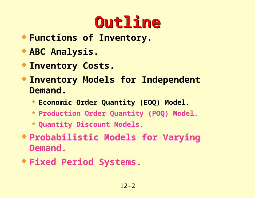
OutlineOutline Functions of Inventory. ABC Analysis. Inventory Costs. Inventory Models for Independent Demand.
Economic Order Quantity (EOQ) Model. Production Order Quantity (POQ) Model. Quantity Discount Models.
Probabilistic Models for Varying Demand. Fixed Period Systems.
12-3
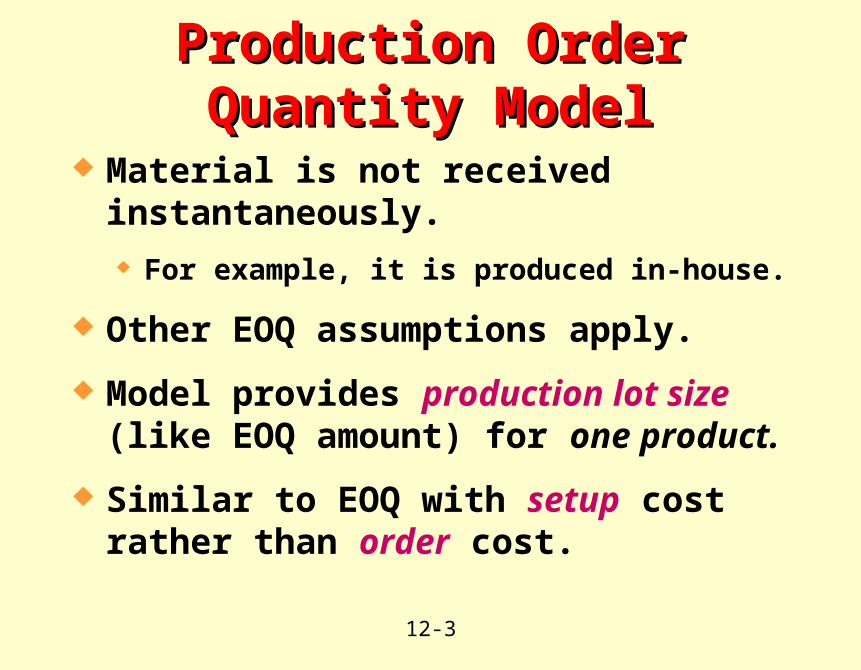
Material is not received instantaneously. For example, it is produced in-house.
Other EOQ assumptions apply.
Model provides production lot size (like EOQ amount) for one product.
Similar to EOQ with setup cost rather than order cost.
Production Order Quantity ModelProduction Order Quantity Model
12-4
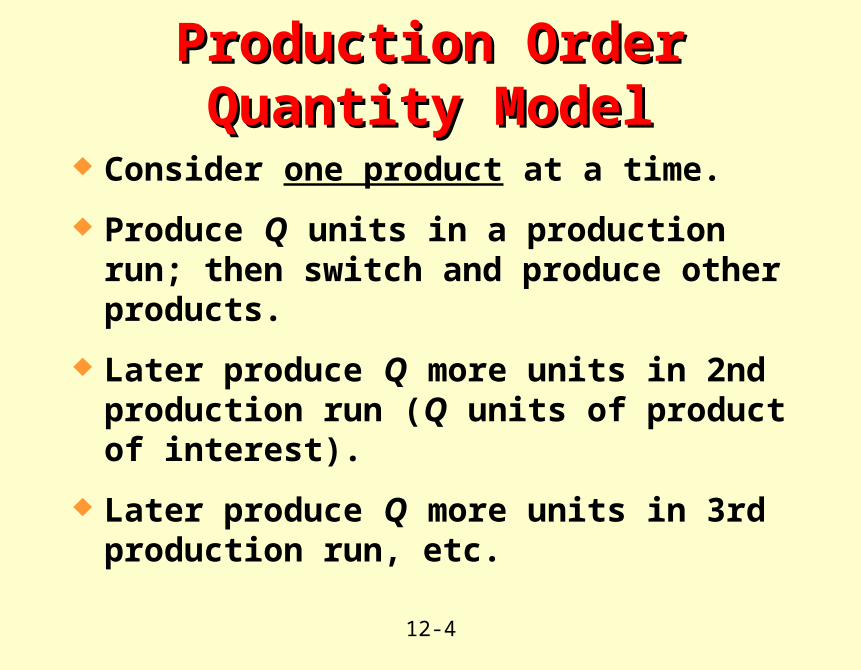
Consider one product at a time.
Produce Q units in a production run; then switch and produce other products.
Later produce Q more units in 2nd production run (Q units of product of interest).
Later produce Q more units in 3rd production run, etc.
Production Order Quantity ModelProduction Order Quantity Model
12-5
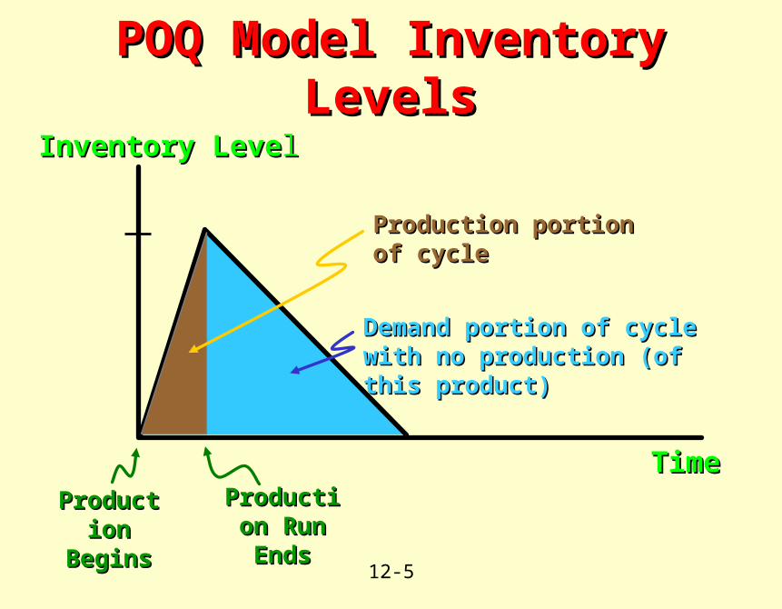
POQ Model Inventory LevelsPOQ Model Inventory Levels
Inventory LeveInventory Levell
TimeTimeProduction Production
BeginsBeginsProduction Production Run EndsRun Ends
Production portion of cycleProduction portion of cycle
Demand portion of cycle with no Demand portion of cycle with no production (of this product)production (of this product)
12-6
POQ Model Inventory LevelsPOQ Model Inventory Levels
Inventory LeveInventory Levell
TimeTimeProduction Production
BeginsBeginsProduction Production Run EndsRun Ends
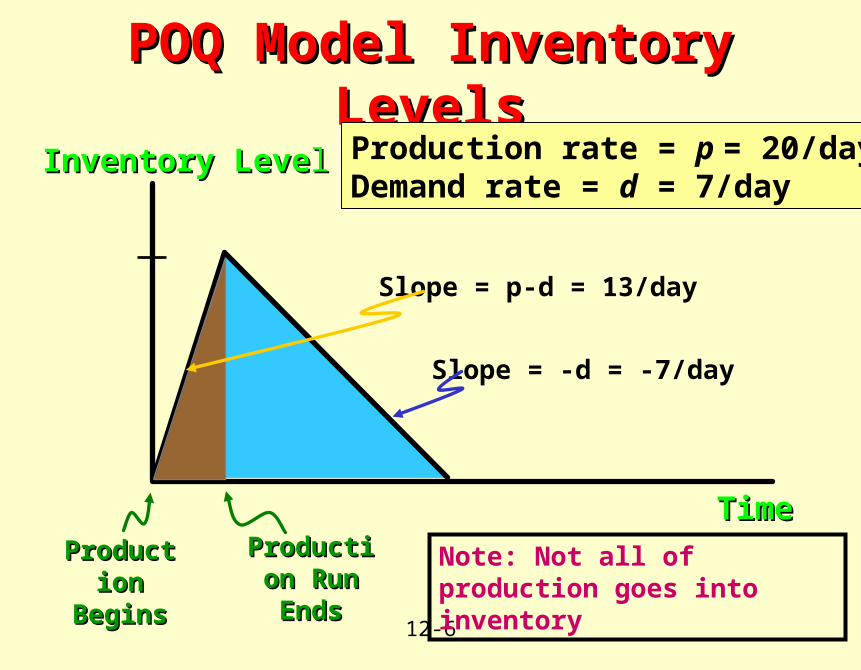
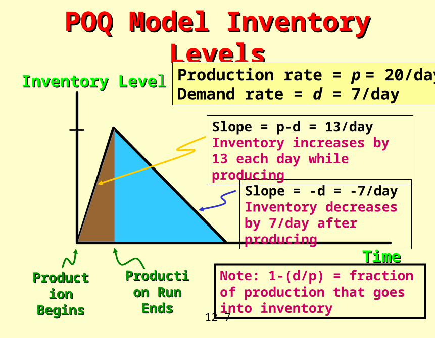
Production rate = p = 20/dayDemand rate = d = 7/day
Slope = -d = -7/day
Slope = p-d = 13/day
Note: Not all of production goes into inventory
12-7
POQ Model Inventory LevelsPOQ Model Inventory Levels
Inventory LeveInventory Levell
TimeTimeProduction Production
BeginsBeginsProduction Production Run EndsRun Ends
Production rate = p = 20/dayDemand rate = d = 7/day
Slope = -d = -7/dayInventory decreases by 7/day after producing
Slope = p-d = 13/dayInventory increases by 13 each day while producing
Note: 1-(d/p) = fraction of production that goes into inventory
12-8
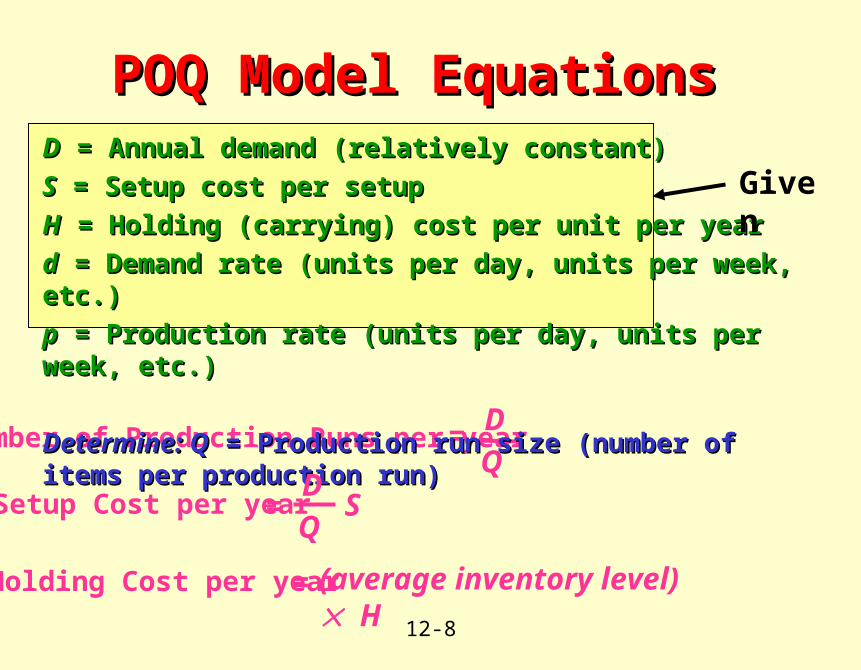
Number of Production Runs per year = D Q
DD = Annual demand (relatively constant) = Annual demand (relatively constant)
SS = Setup cost per setup = Setup cost per setup
HH = Holding (carrying) cost per unit per year = Holding (carrying) cost per unit per year
dd = Demand rate (units per day, units per week, etc.) = Demand rate (units per day, units per week, etc.)
pp = Production rate (units per day, units per week, etc.) = Production rate (units per day, units per week, etc.)
Determine: QDetermine: Q = Production run size (number of items per production run) = Production run size (number of items per production run)
POQ Model Equations POQ Model Equations
Setup Cost per year = SD
Q
Holding Cost per year = (average inventory level) H
Given

12-9
POQ Model Inventory LevelsPOQ Model Inventory Levels
TimeTime
Inventory LevelInventory Level
Production Production Portion of CyclePortion of Cycle
Maximum Inventory Maximum Inventory = Q(1-(d/p))= Q(1-(d/p))
Demand portion of cycle with no supply
12-10
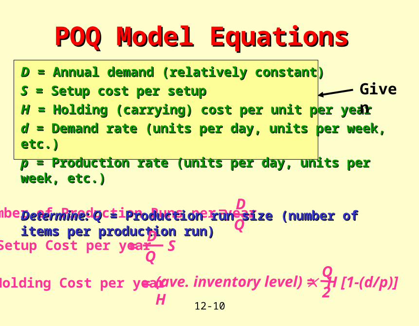
Number of Production Runs per year = D Q
DD = Annual demand (relatively constant) = Annual demand (relatively constant)
SS = Setup cost per setup = Setup cost per setup
HH = Holding (carrying) cost per unit per year = Holding (carrying) cost per unit per year
dd = Demand rate (units per day, units per week, etc.) = Demand rate (units per day, units per week, etc.)
pp = Production rate (units per day, units per week, etc.) = Production rate (units per day, units per week, etc.)
Determine: QDetermine: Q = Production run size (number of items per production run) = Production run size (number of items per production run)
POQ Model Equations POQ Model Equations
Setup Cost per year = SD
Q
Holding Cost per year = (ave. inventory level) H
Given
= H [1-(d/p)]Q 2
12-11
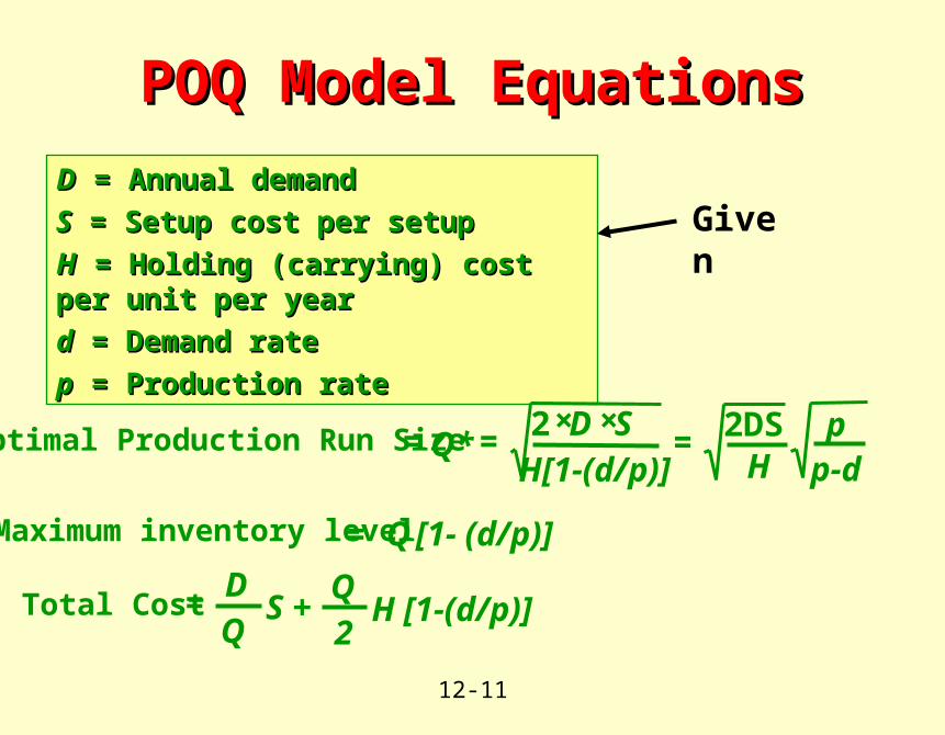
Optimal Production Run Size =
Maximum inventory level = Q [1- (d/p)]
DD = Annual demand = Annual demand
SS = Setup cost per setup = Setup cost per setup
HH = Holding (carrying) cost per unit per year = Holding (carrying) cost per unit per year
dd = Demand rate = Demand rate
pp = Production rate = Production rate
POQ Model EquationsPOQ Model Equations
Total Cost = D Q
S + Q
2H [1-(d/p)]
=× ×
Q*D S
H[1-(d/p)]2 =
H2DS
p-dp
Given
12-12
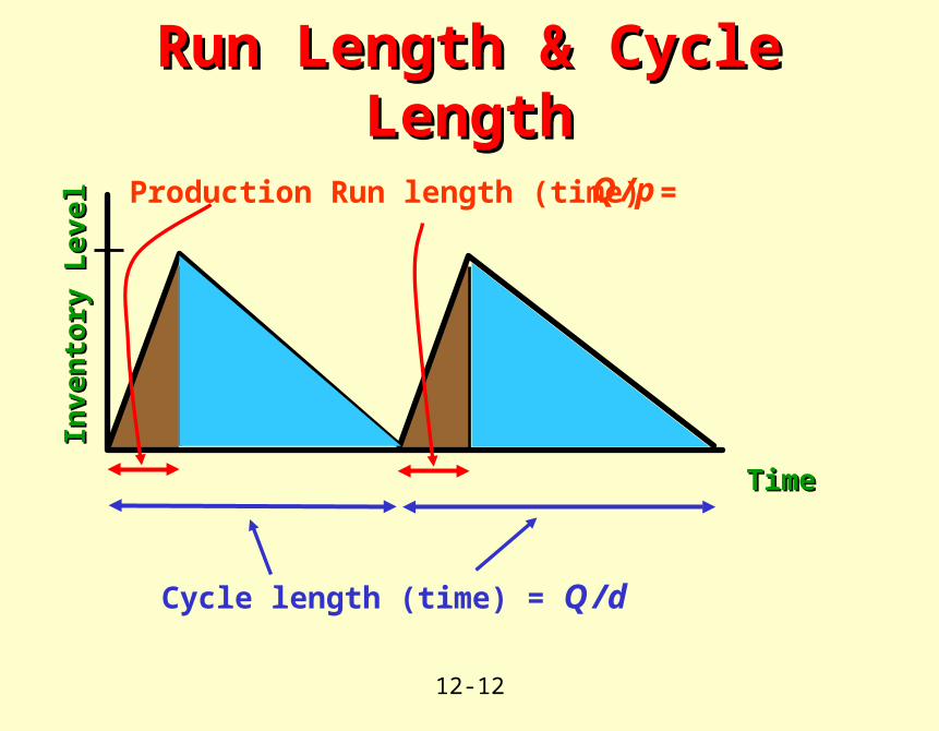
Run Length & Cycle LengthRun Length & Cycle Length
TimeTime
Inve
ntor
y Le
vel
Inve
ntor
y Le
vel
Production Run length (time) = Q /p
Cycle length (time) = Q /d
12-13
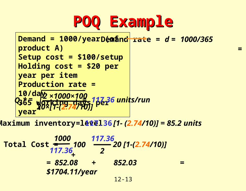
POQ ExamplePOQ ExampleDemand = 1000/year (of product A)Setup cost = $100/setupHolding cost = $20 per year per itemProduction rate = 10/day365 working days per year
2 ×1000×100=Qp*20×[1-(2.74/10)]
= 117.36 units/run
Total Cost = 1000
117.36 100 +
117.36
220 [1-(2.74/10)]
Maximum inventory level = 117.36 [1- (2.74/10)] = 85.2 units
Demand rate = d = 1000/365 = 2.74/day
= 852.08 + 852.03 = $1704.11/year
12-14
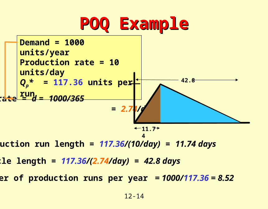
POQ ExamplePOQ ExampleDemand = 1000 units/yearProduction rate = 10 units/dayQp* = 117.36 units per run
Demand rate = d = 1000/365 = 2.74/day
Number of production runs per year = 1000/117.36 = 8.52
Cycle length = 117.36/(2.74/day) = 42.8 days
Production run length = 117.36/(10/day) = 11.74 days
11.74
42.8
12-15
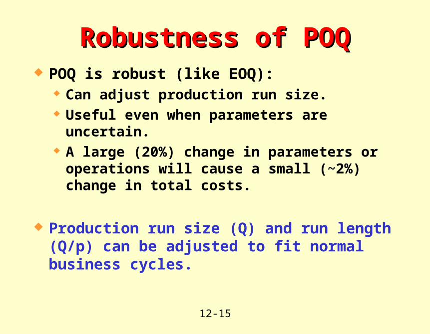
POQ is robust (like EOQ): Can adjust production run size. Useful even when parameters are uncertain. A large (20%) change in parameters or operations
will cause a small (~2%) change in total costs.
Production run size (Q) and run length (Q/p) can be adjusted to fit normal business cycles.
Robustness of POQRobustness of POQ
12-16
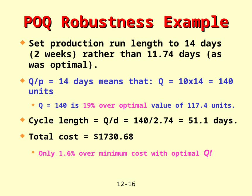
Set production run length to 14 days (2 weeks) rather than 11.74 days (as was optimal).
Q/p = 14 days means that: Q = 10x14 = 140 units
Q = 140 is 19% over optimal value of 117.4 units.
Cycle length = Q/d = 140/2.74 = 51.1 days.
Total cost = $1730.68
Only 1.6% over minimum cost with optimal Q!
POQ Robustness ExamplePOQ Robustness Example
12-17
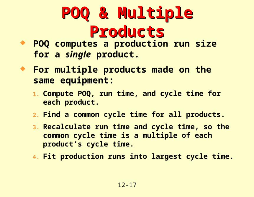
POQ computes a production run size for a single product.
For multiple products made on the same equipment:1. Compute POQ, run time, and cycle time for each product.
2. Find a common cycle time for all products.
3. Recalculate run time and cycle time, so the common cycle time is a multiple of each product’s cycle time.
4. Fit production runs into largest cycle time.
POQ & Multiple ProductsPOQ & Multiple Products
12-18
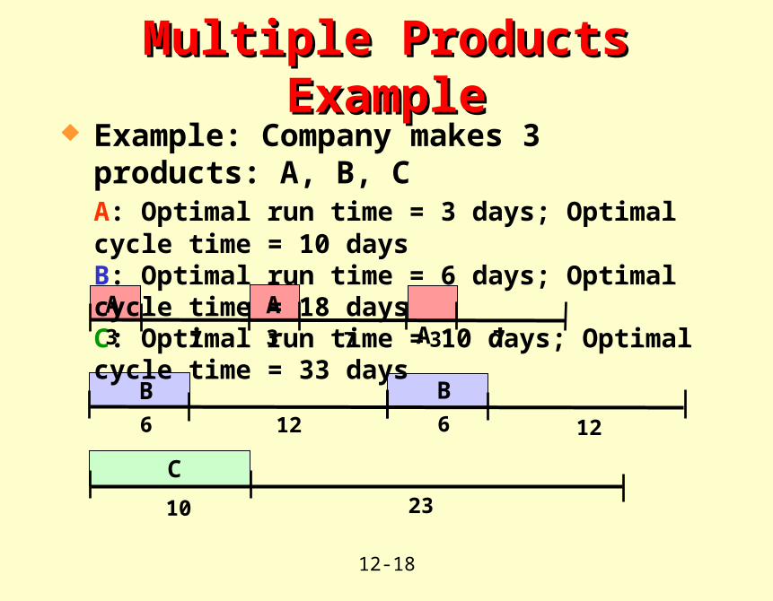
Example: Company makes 3 products: A, B, CA: Optimal run time = 3 days; Optimal cycle time = 10 days B: Optimal run time = 6 days; Optimal cycle time = 18 days C: Optimal run time = 10 days; Optimal cycle time = 33 days
Multiple Products ExampleMultiple Products Example
10 23
C
3 7 7 7 33
A AA
126 12
B6
B
12-19
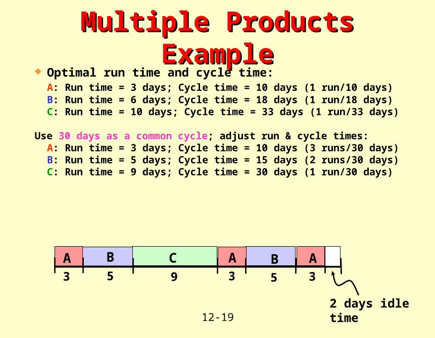
Optimal run time and cycle time:A: Run time = 3 days; Cycle time = 10 days (1 run/10 days)B: Run time = 6 days; Cycle time = 18 days (1 run/18 days)C: Run time = 10 days; Cycle time = 33 days (1 run/33 days)
Use 30 days as a common cycle; adjust run & cycle times:A: Run time = 3 days; Cycle time = 10 days (3 runs/30 days)B: Run time = 5 days; Cycle time = 15 days (2 runs/30 days)C: Run time = 9 days; Cycle time = 30 days (1 run/30 days)
Multiple Products ExampleMultiple Products Example
3 5 9 5 33
A B C B AA
2 days idle time
12-20
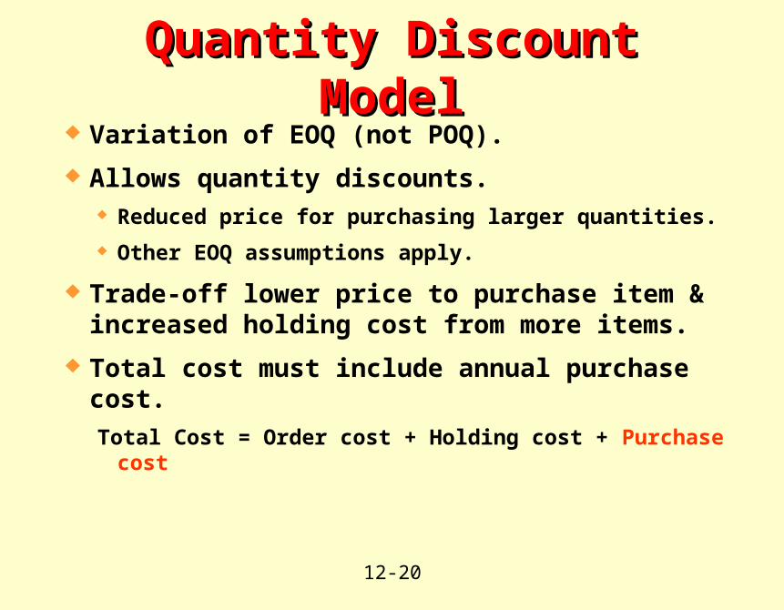
Variation of EOQ (not POQ).
Allows quantity discounts. Reduced price for purchasing larger quantities.
Other EOQ assumptions apply.
Trade-off lower price to purchase item & increased holding cost from more items.
Total cost must include annual purchase cost.
Total Cost = Order cost + Holding cost + Purchase cost
Quantity Discount ModelQuantity Discount Model
12-21
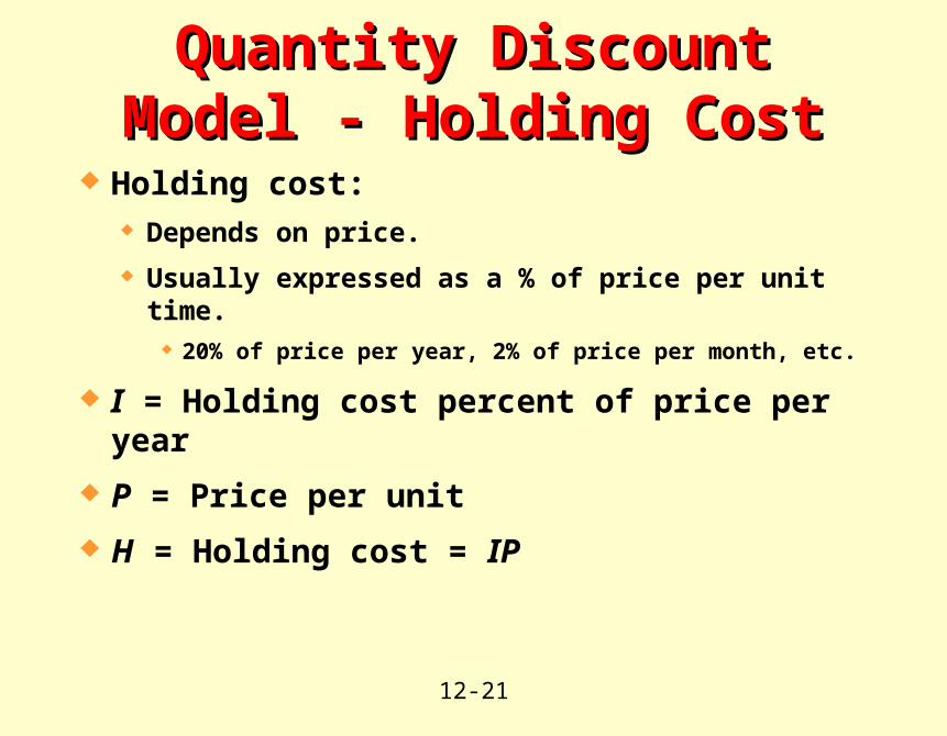
Holding cost: Depends on price.
Usually expressed as a % of price per unit time. 20% of price per year, 2% of price per month, etc.
I = Holding cost percent of price per year
P = Price per unit
H = Holding cost = IP
Quantity Discount Model - Holding Quantity Discount Model - Holding CostCost
12-22
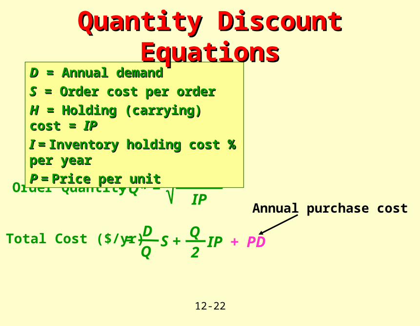
Order Quantity = =× ×
Q*D SIP
2
DD = Annual demand = Annual demand
SS = Order cost per order = Order cost per order
HH = Holding (carrying) cost = = Holding (carrying) cost = IPIP
I = I = Inventory holding cost % per yearInventory holding cost % per year
P = P = Price per unitPrice per unit
Quantity Discount EquationsQuantity Discount Equations
Total Cost ($/yr) = D Q
S + Q
2IP + PD
Annual purchase cost
12-23
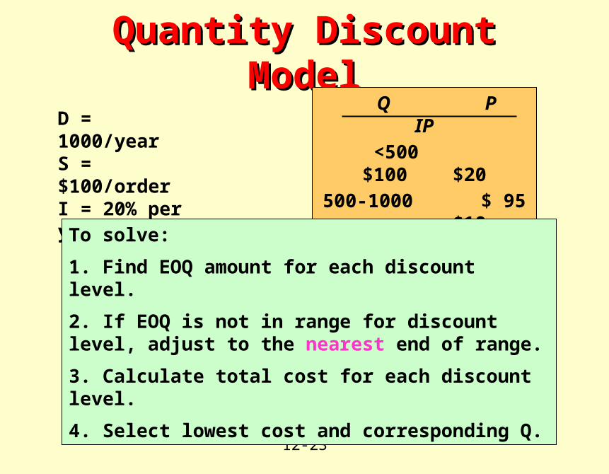
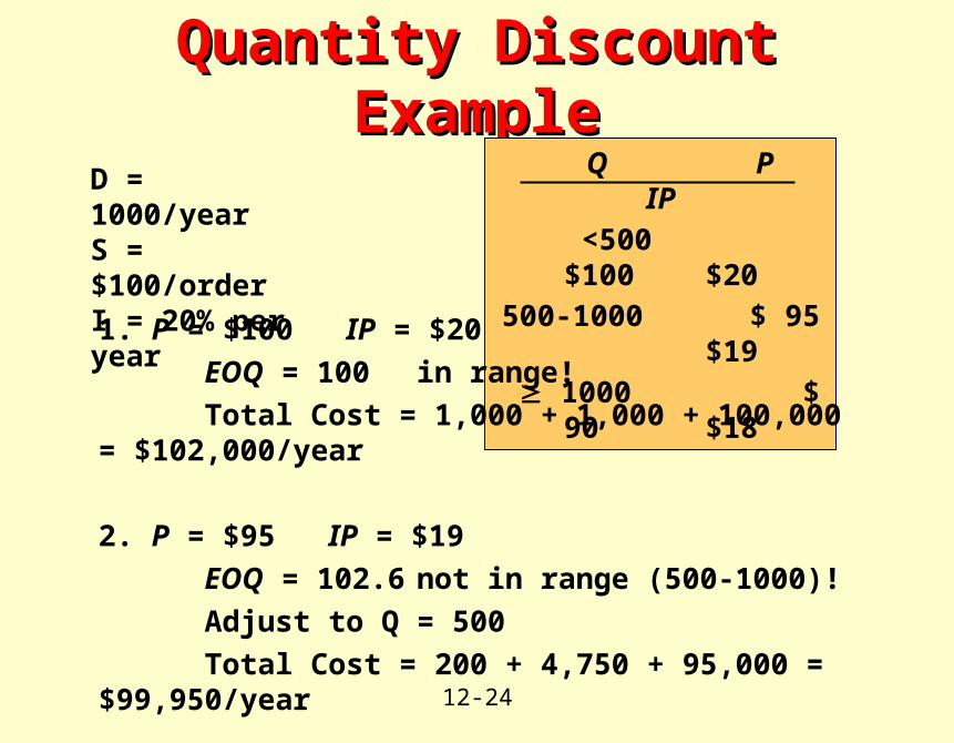
Quantity Discount ModelQuantity Discount Model
D = 1000/yearS = $100/orderI = 20% per year
Q P IP <500 $100 $20500-1000 $ 95 $19 1000 $ 90 $18
To solve:
1. Find EOQ amount for each discount level.
2. If EOQ is not in range for discount level, adjust to the nearest end of range.
3. Calculate total cost for each discount level.
4. Select lowest cost and corresponding Q.
12-24
Quantity Discount ExampleQuantity Discount Example
D = 1000/yearS = $100/orderI = 20% per year
Q P IP <500 $100 $20500-1000 $ 95 $19 1000 $ 90 $18
1. P = $100 IP = $20
EOQ = 100 in range!
Total Cost = 1,000 + 1,000 + 100,000 = $102,000/year
2. P = $95 IP = $19
EOQ = 102.6 not in range (500-1000)!
Adjust to Q = 500
Total Cost = 200 + 4,750 + 95,000 = $99,950/year
12-25
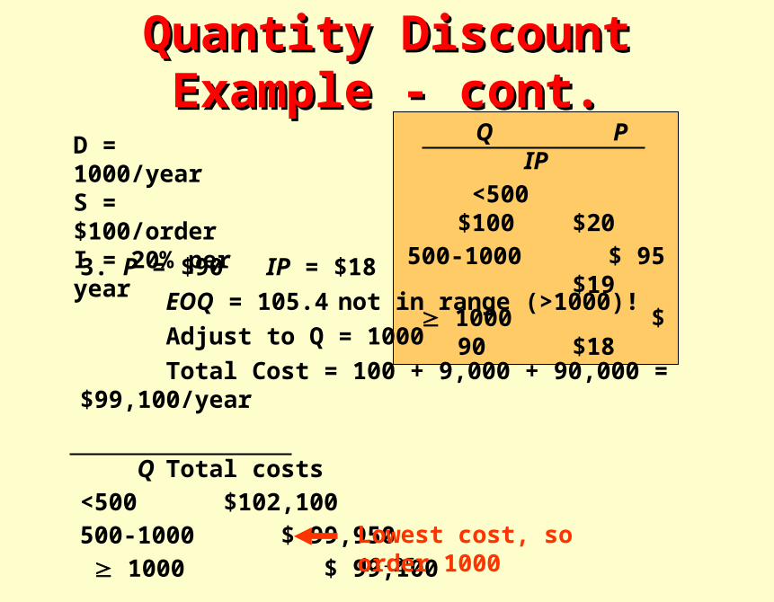
Quantity Discount Example - cont.Quantity Discount Example - cont.
D = 1000/yearS = $100/orderI = 20% per year
Q P IP <500 $100 $20500-1000 $ 95 $19 1000 $ 90 $18
3. P = $90 IP = $18
EOQ = 105.4 not in range (>1000)!
Adjust to Q = 1000
Total Cost = 100 + 9,000 + 90,000 = $99,100/year
Q Total costs<500 $102,100500-1000 $ 99,950 1000 $ 99,100 Lowest cost, so order 1000
12-26
In basic EOQ model, demand and lead time are known and constant, so there should never be a stockout.
If demand or lead time vary, then may have a stockout: Due to larger than expected demand.
Due to longer than expected lead time.
StockoutsStockouts
12-27
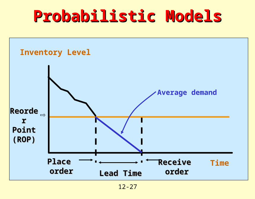
Probabilistic ModelsProbabilistic Models
Reorder Reorder Point Point (ROP)(ROP)
Time
Inventory Level
Lead TimeLead Time
Place Place orderorder
Receive Receive orderorder
Average demand
12-28
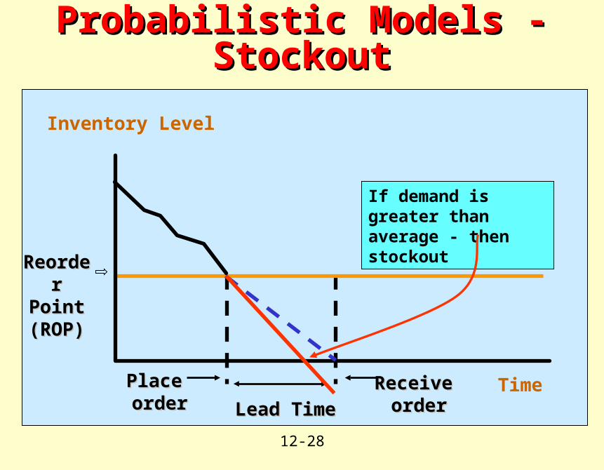
Probabilistic Models - StockoutProbabilistic Models - Stockout
Reorder Reorder Point Point (ROP)(ROP)
Time
Inventory Level
Lead TimeLead Time
Place Place orderorder
Receive Receive orderorder
If demand is greater than average - then stockout
12-29
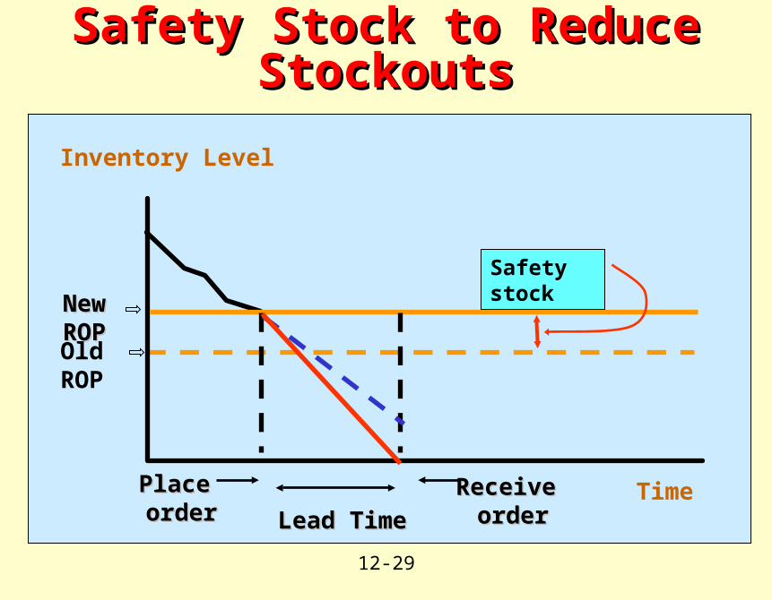
Safety Stock to Reduce StockoutsSafety Stock to Reduce Stockouts
Time
Inventory Level
Lead TimeLead Time
Place Place orderorder
Receive Receive orderorder
Safety stock
New ROPNew ROP
Old ROP
12-30
Safety stock is inventory held to protect against stockout.
Service level = 1 - Probability of stockout
Service level of 95% means 5% chance of stockout.
Higher service level means more safety stock.
More safety stock means higher ROP. ROP = Expected demand during lead time + Safety stock
Safety Stock & Service LevelSafety Stock & Service Level
12-31
Demand follows normal distribution. d = Average demand rate per day.
= Standard deviation of demand.
ROP = d L + safety stock
safety stock = ss = Z
Z is from Standard Normal Table in Appendix I.
Probabilistic ModelsProbabilistic Models
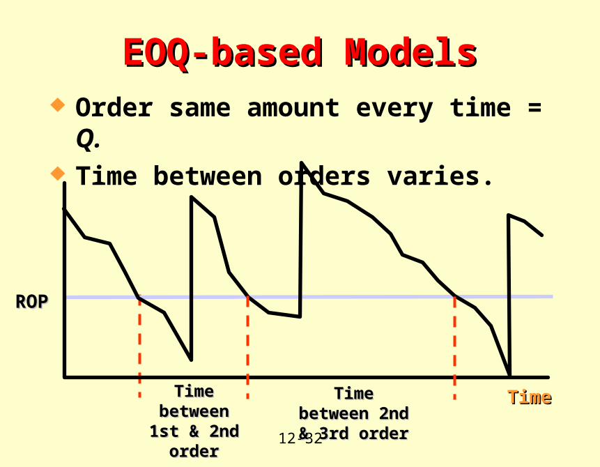
12-32
Order same amount every time = Q. Time between orders varies.
EOQ-based ModelsEOQ-based Models
ROPROP
TimeTimeTime between Time between 1st & 2nd order1st & 2nd order
Time between 2nd Time between 2nd & 3rd order& 3rd order
12-33
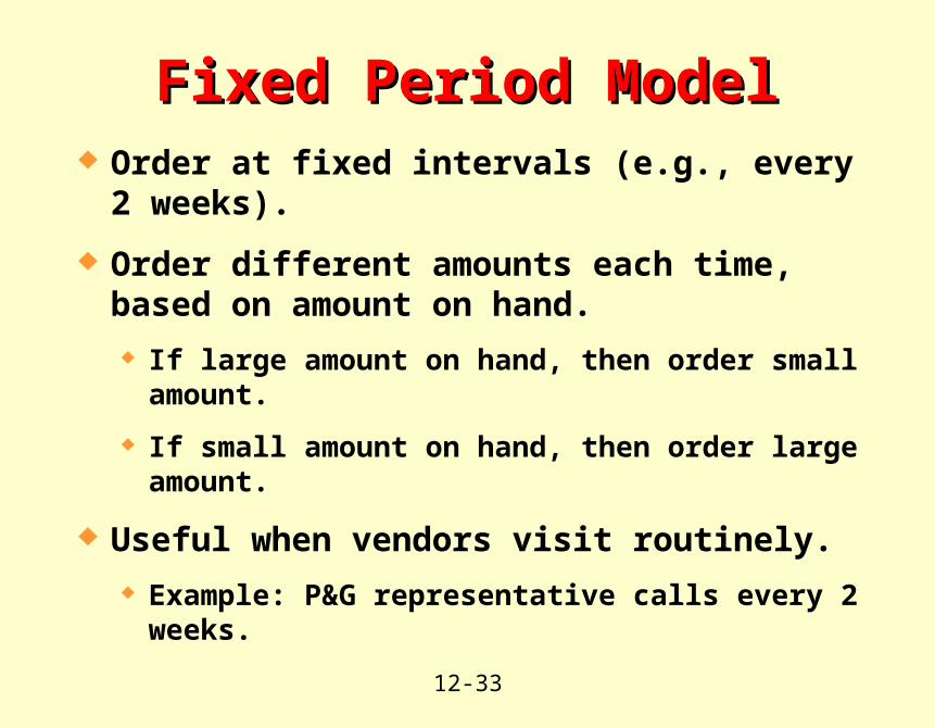
Order at fixed intervals (e.g., every 2 weeks).
Order different amounts each time, based on amount on hand.
If large amount on hand, then order small amount.
If small amount on hand, then order large amount.
Useful when vendors visit routinely.
Example: P&G representative calls every 2 weeks.
Fixed Period ModelFixed Period Model
12-34
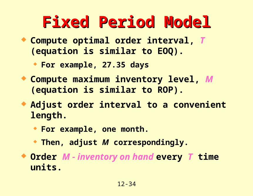
Compute optimal order interval, T (equation is similar to EOQ). For example, 27.35 days
Compute maximum inventory level, M (equation is similar to ROP).
Adjust order interval to a convenient length. For example, one month.
Then, adjust M correspondingly.
Order M - inventory on hand every T time units.
Fixed Period ModelFixed Period Model
12-35
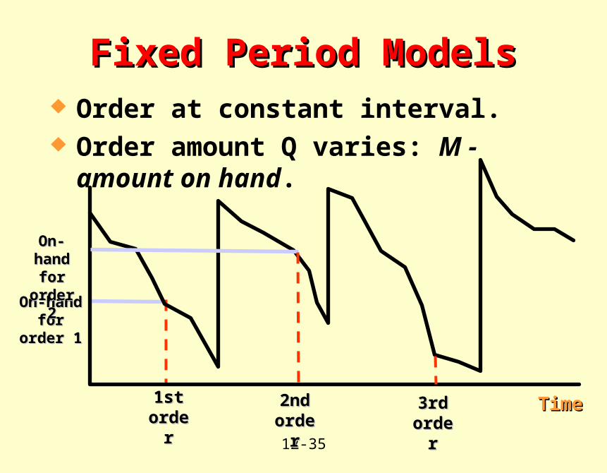
Order at constant interval. Order amount Q varies: M - amount on hand.
Fixed Period ModelsFixed Period Models
On-hand On-hand for order 1for order 1
TimeTime1st 1st orderorder
2nd 2nd orderorder
3rd 3rd orderorder
On-hand On-hand for order 2for order 2