10-708: Probabilistic Graphical Models 10-708, Spring 2013

12 : HMM & CRF

Lecturer: Eric P. Xing Scribes: Salim Akhter Chowdhury, Jingwei Zhang

1 Introduction

Conditional Random Field (CRF) is one of the most important graphical models in literature. It is proposedto overcome some of the drawbacks of Hidden Markov Model (HMM). This lectures first revisits the HMM,briefly introduces the MEMM, then explains the inference and learning algorithm in CRF.

2 Hidden Markov Model Revisit

A hidden Markov model (HMM) is a statistical Markov model in which the system being modeled is assumedto be a Markov process with unobserved (hidden) states.

Figure 1: HMM

2.1 Parameterization

Assume the HMM shown in figure 1 has M different states, and K possible observations. Then this HMMis defined by three parameters:

πi = P (yi1 = 1)

ai,j = P (yjt = 1|yit−1 = 1)

bi,k = P (xkt = 1|yit = 1)

Where πi is the prior probability of the initial state being state i; a is the transition matrix, with ai,j beingthe transition probability from state i to state j; b is the emission matrix, with bi,k being the emissionprobability of observation k at state i.

1

2 12 : HMM & CRF

2.2 Inference

When all the three parameters are known, inference can be done using forward and backward algorithm.

Forward algorithm:

• Initialization:αk1 = P (x1|yk1 = 1)πk

• Iteration:αkt = P (xt|ykt = 1)

∑i

αit−1ai,k

• Termination:P (x) =

∑k

αkT

Backward algorithm:

• Initialization:βkT = 1,∀k

• Iteration:βkt =

∑i

ak,iP (xt+1|yit+1 = 1)βit+1

• Termination:P (x) =

∑k

αk1βk1

2.3 Learning

When not all of the parameters are known, learning has to be conducted to get the hidden variables. Thereare mainly two types of learning:

• Supervised learning: estimation when the right answer is knownIf we know the true state path then Maximum Likelihood (ML) parameter estimation would be trivial.

aMLij =

#(i→ j)

#(i→ •)=

∑n

∑Tt=2 y

in,t−1y

jn,t∑

n

∑Tt=2 y

in,t−1

bMLik =

#(i→ k)

#(i→ •)=

∑n

∑Tt=1 y

in,tx

kn,t∑

n

∑Tt=1 y

in,t

• Unsurpervised learning: estimation when the right answer is unknownWhen the true state path is unknown, we can fill in the missing values using inference recursions, e.g.,Expectation Maximization (EM), in the E step of which the expected value of the hidden variables arecomputed, then in the M step inference is conducted as in the supervised learning case.

12 : HMM & CRF 3

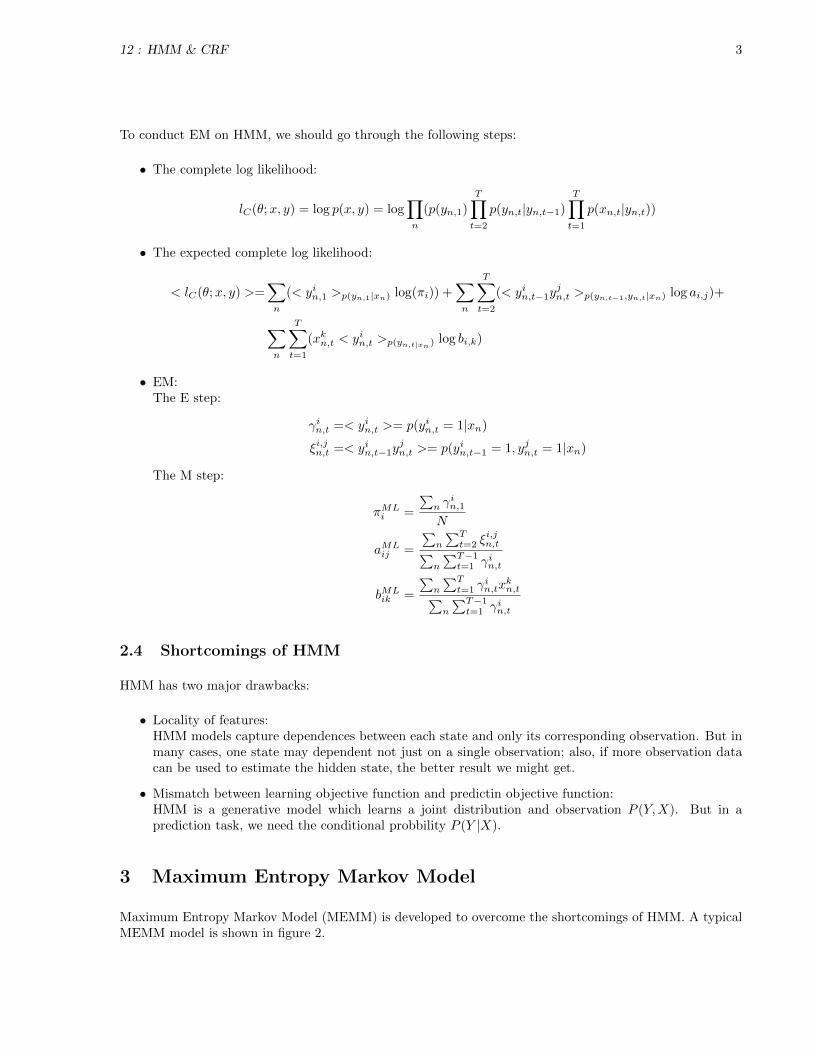
To conduct EM on HMM, we should go through the following steps:

• The complete log likelihood:

lC(θ;x, y) = log p(x, y) = log∏n

(p(yn,1)

T∏t=2

p(yn,t|yn,t−1)

T∏t=1

p(xn,t|yn,t))

• The expected complete log likelihood:

< lC(θ;x, y) >=∑n

(< yin,1 >p(yn,1|xn) log(πi)) +∑n

T∑t=2

(< yin,t−1yjn,t >p(yn,t−1,yn,t|xn) log ai,j)+

∑n

T∑t=1

(xkn,t < yin,t >p(yn,t|xn ) log bi,k)

• EM:The E step:

γin,t =< yin,t >= p(yin,t = 1|xn)

ξi,jn,t =< yin,t−1yjn,t >= p(yin,t−1 = 1, yjn,t = 1|xn)

The M step:

πMLi =

∑n γ

in,1

N

aMLij =

∑n

∑Tt=2 ξ

i,jn,t∑

n

∑T−1t=1 γin,t

bMLik =

∑n

∑Tt=1 γ

in,tx

kn,t∑

n

∑T−1t=1 γin,t

2.4 Shortcomings of HMM

HMM has two major drawbacks:

• Locality of features:HMM models capture dependences between each state and only its corresponding observation. But inmany cases, one state may dependent not just on a single observation; also, if more observation datacan be used to estimate the hidden state, the better result we might get.

• Mismatch between learning objective function and predictin objective function:HMM is a generative model which learns a joint distribution and observation P (Y,X). But in aprediction task, we need the conditional probbility P (Y |X).

3 Maximum Entropy Markov Model

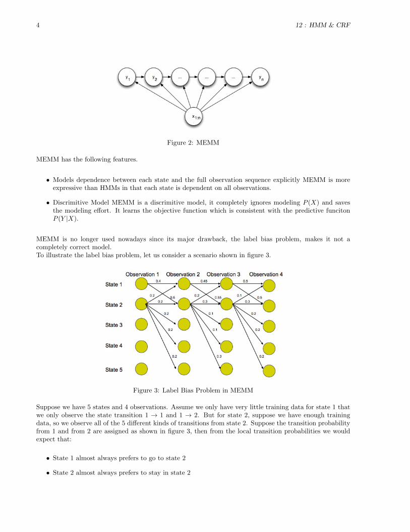
Maximum Entropy Markov Model (MEMM) is developed to overcome the shortcomings of HMM. A typicalMEMM model is shown in figure 2.

4 12 : HMM & CRF

Figure 2: MEMM

MEMM has the following features.

• Models dependence between each state and the full observation sequence explicitly MEMM is moreexpressive than HMMs in that each state is dependent on all observations.

• Discrimitive Model MEMM is a discrimitive model, it completely ignores modeling P (X) and savesthe modeling effort. It learns the objective function which is consistent with the predictive funcitonP (Y |X).

MEMM is no longer used nowadays since its major drawback, the label bias problem, makes it not acompletely correct model.To illustrate the label bias problem, let us consider a scenario shown in figure 3.

Figure 3: Label Bias Problem in MEMM

Suppose we have 5 states and 4 observations. Assume we only have very little training data for state 1 thatwe only observe the state transition 1 → 1 and 1 → 2. But for state 2, suppose we have enough trainingdata, so we observe all of the 5 different kinds of transitions from state 2. Suppose the transition probabilityfrom 1 and from 2 are assigned as shown in figure 3, then from the local transition probabilities we wouldexpect that:

• State 1 almost always prefers to go to state 2

• State 2 almost always prefers to stay in state 2

12 : HMM & CRF 5

But if compute the probability of following paths, we would get that:

• 1→ 1→ 1→ 1 : 0.4× 0.45× 0.5 = 0.09

• 2→ 2→ 2→ 2 : 0.2× 0.3× 0.3 = 0.018

• 1→ 2→ 1→ 2 : 0.6× 0.2× 0.5 = 0.06

• 1→ 1→ 2→ 2 : 0.4× 0.55× 0.3 = 0.066

From the probabilities above, we get that the most likely path is 1 → 1 → 1 → 1, which is not consistentwith our expectation that state 1 wants to go to state 2 and state 2 wants to remain in state 2. This isbecause that from our limited observation, state 1 has only two transitions but state 2 has 5, so the averageprobability from state 2 is lower. This problem makes the MEMM prefer the states with lower number oftransitions over others.

The solution to this problem is to not normalize probabilities locally, but globally, which brings us fromthe local probabilities to local potentials, so that the states with lower transitions do not have an unfairadvantage.

4 CRF

4.1 From MEMM to CRF

From the analysis from above, CRF is introduced to solve the problem of local bias of MEMM.For MEMM, the posterior distribution can be read from figure 2:

P (y1:n|x1:n) =

n∏i=1

P (yi|yi−1, x1:n) =

n∏i=1

exp(wT f(yi, yi−1, x1:n))

Z(yi−1, x1:n)

For CRF, this posterior changes to:

P (y1:n|x1:n) =1

Z(x1:n)

n∏i=1

φ(yi, yi−1, x1:n) =1

Z(x1:n, w)

n∏i=1

exp(wT f(yi, yi−1, x1:n))

Which correspondes to the graphical model shown in figure 4.

Figure 4: CRF

From the model we can see that CRF is a partially directed model:

6 12 : HMM & CRF

• CRF is a discriminative model like MEMM

• The usage of global normalizer Z(x) overcomes the label bias problem of MEMM

• CRF models the dependence between each state and the entire observation sequence (like MEMM)

5 General Parametric Form of CRF

The general parametric form of CRF is

P (y|x) =1

Z(x, λ, µ)exp(

n∑i=1

(∑k

λkfk(yi, yi−1,x) +∑l

µlgl(yi,x)))

=1

Z(x, λ, µ)exp(

n∑i=1

(λT f(yi, yi−1,x) + µTg(yi,x)))

where

Z(x, λ, µ) =∑y

exp(

n∑i=1

(λT f(yi, yi−1,x) + µTg(yi,x)))

6 Inference in CRF

The inference problem in CRF can be stated as :“Given CRF parameters λ and µ, find the vector y∗ thatmaximizes the posterior probability P (y|x)”. This statement can be expressed more concretely as:

y∗ = arg maxy

exp(

n∑i=1

(λT f(yi, yi−1,x) + µTg(yi,x)))

The partition function Z(x) can be ignored here because it is not a function of y.

In order to find the optimum parameter values, max-product algorithm can be run on the junction tree ofCRF which is the same as Viterbi decoding used in HMM. The clique tree for the CRF in figure 4 is shownin figure 5.

Figure 5: Clique tree for the CRF in figure 4

12 : HMM & CRF 7

7 Learning in CRF

The parameter learning process in CRF can be formulated as: Given (xd,yd)Nd=1, find λ∗, µ∗, such that:

λ∗, µ∗ = arg maxλ,µ

L(λ, µ)

= arg maxλ,µ

N∏d=1

P (yd|xd, λ, µ)

= arg maxλ,µ

N∏d=1

1

Z(xd, λ, µ)exp(

n∑i=1

(λT f(yd,i, yd,i−1,xd) + µTg(yd,i,xd)))

= arg maxλ,µ

N∑d=1

(

N∑i=1

(λT f(yd,i, yd,i−1,xd) + µTg(yd,i,xd))− logZ(xd, λ, µ))

Now, if we take the derivative with respect to λ, we get

∇λL(λ, µ) =

N∑d=1

(

N∑i=1

(f(yd,i, yd,i−1,xd)−∑y

(P (y|xd)N∑i=1

f(yd,i, yd,i−1,xd))))

From the final term in the above equation, we see that gradient of the log-partition function in an exponentialfamily is the expectation of the sufficient statistics. It can be written as:

∑y

(P (y|xd)N∑i=1

f(yi, yi−1,xd)) =

N∑i=1

(∑y

f(yi, yi−1,xd)P (y|xd))

=

N∑i=1

∑yi,yi−1

f(yi, yi−1,xd)P (yi, yi−1|xd)

The expectation is over the corresponding marginal probability of neighboring nodes. For each data point,we have to run forward backward algorithm, so learning is very expensive. Although computing the modelexpectation requires exponentially large number of summations, it is tractable for trees and chains, since themarginals can be computed using the sum-product algorithm.

We now describe here how the marginals can be computed using junction-tree calibration.

• Junction Tree Initialization:

α0(yi, yi−1) = exp(λT f(yi, yi−1,xd) + µTg(yi,xd))

• After Junction Tree Calibration:P (yi, yi−1|xd) ∝ α(yi, yi−1)

which implies

P (yi, yi−1|xd) =α(yi, yi−1)∑

yi,yi−1α(yi, yi−1)

= α′(yi, yi−1)

8 12 : HMM & CRF

Computing the feature expectations using calibrated potentials results in

∑yi,yi−1

f(yi, yi−1,xd)P (yi, yi−1|xd) =∑

yi,yi−1

f(yi, yi−1,xd)α′(yi, yi−1)

Now, if we take derivative of L(λ, µ) with respect to λ, we get

∇λL(λ, µ) =

N∑d=1

(

N∑i=1

(f(yd,i, yd,i−1,xd)−∑y

(P (y|xd)N∑i=1

f(yd,i, yd,i−1,xd))))

=

N∑d=1

(

N∑i=1

(f(yd,i, yd,i−1,xd)−∑

yi,yi−1

α′(yi, yi−1)f(yd,i, yd,i−1,xd)))

Now, we can use gradient ascent to find the optimal value of λ and µ. The update equations are:

λ(t+1) = λ(t) + η∇λL(λ(t), µ(t))

µ(t+1) = µ(t) + η∇µL(λ(t), µ(t))

In practice, a Gaussian Regularizer for the parameter vector is used to improve generalizability. The objectivefunction looks like the following in that case:

λ∗, µ∗ = arg maxλ,µ

N∑d=1

logP (yd|xd, λ, µ)− 1

2σ2(λTλ+ µTµ)

We have to do inference for each sample at each iteration, so gradient descent can be very slow in practice.Two widely used alternatives to gradient descent are Conjugate Gradient method and Limited MemoryQuasi-Newton method.

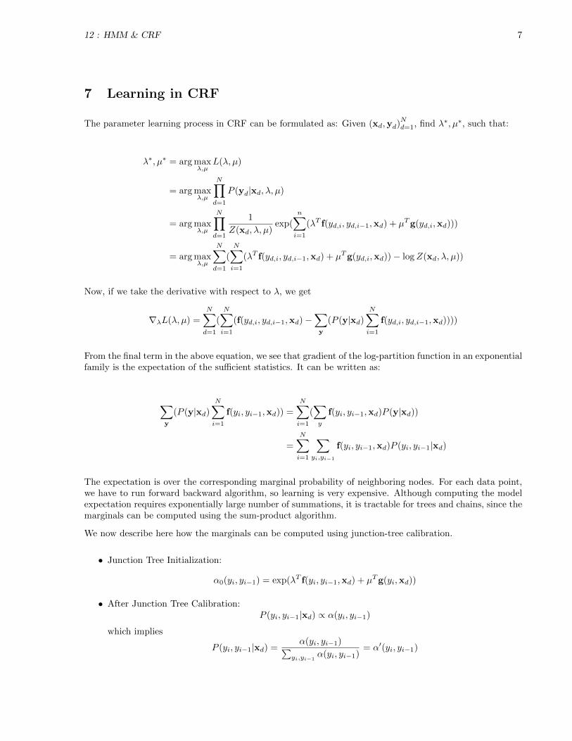
A comparison of error rates among HMM, MEMM and CRF on randomly generated synthetic data is shownin figure 6. In that figure, the top left and top right plot show that MEMM is outperformed by CRFand HMM respectively. The bottom plot shows that when data is of higher order (represented with solidcircle in that plot), CRF outperforms HMM. This is because, in CRF, each hidden state is dependent onmultiple observations, whereas in HMM, each hidden state depends on only one observation. So, higherorder dependencies cannot be captured by HMM.

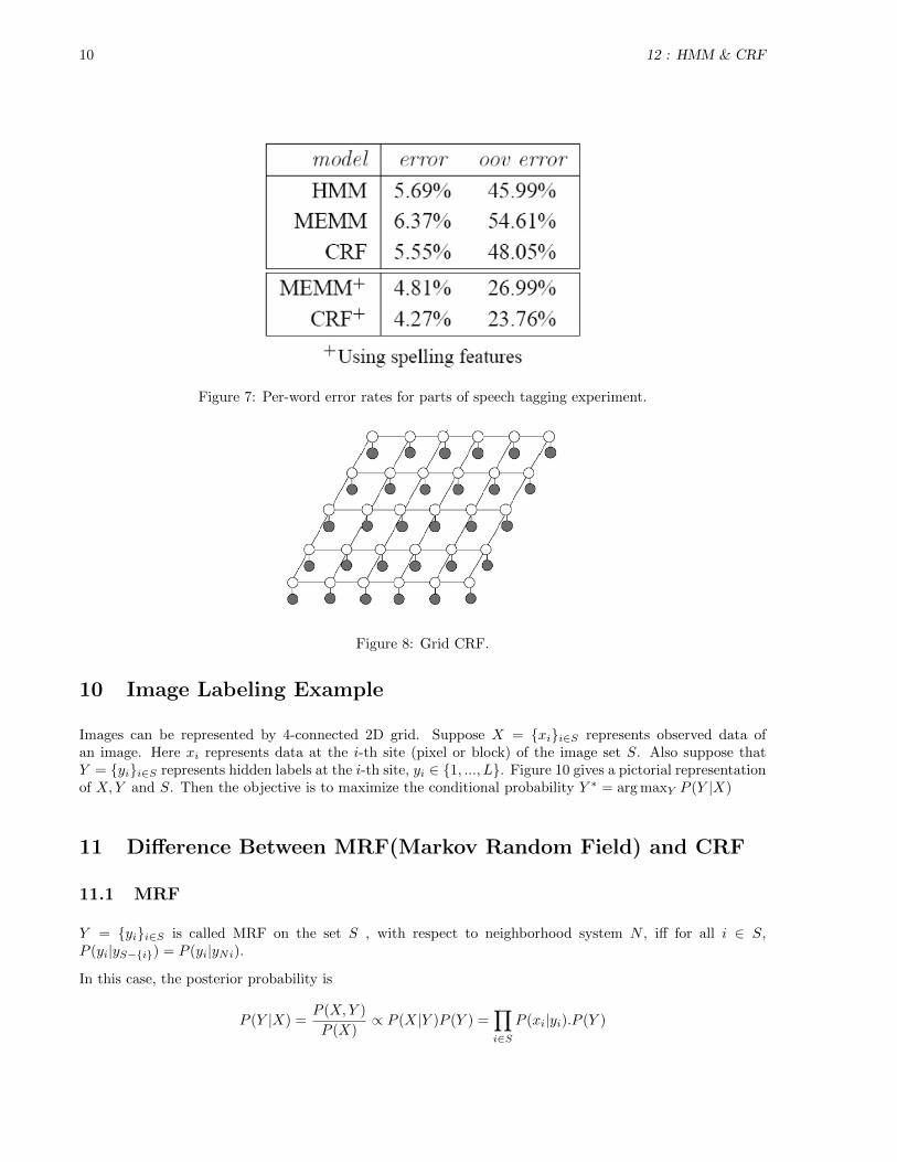
Results from a parts of speech tagging experiments is shown in figure 7. In this experiment, each word in agiven input sentence is labelled with one of 45 syntactic tags. Two sets of experiments were performed withthis natural language data. In the first case, first order HMM, MEMM and CRF models are used. Heretoo, HMM outperforms MEMM and CRF outperforms HMM. Now when additional spelling features areused (i.e. presence of upper case letter in the beginning of a word, presence of hyphens etc), both CRF andMEMM take advantage of these features, with overall error rate get reduced by around 25%.

8 Other CRFs

Until now, we have discussed only one dimensional CRFs which are chains. Inference and learning are exacton these graphs. However, we can have more complex CRFs, like grid CRFs(figure 8), where inference

12 : HMM & CRF 9

Figure 6: Error rates for HMM, CRF and MEMM on randomly generated synthetic datasets.

and learning are no longer tractable. Approximate inference techniques like MCMC sampling, VariationalInference and Loopy Belief Propagation are used for such CRFs. These techniques will be discussed later inthe course.

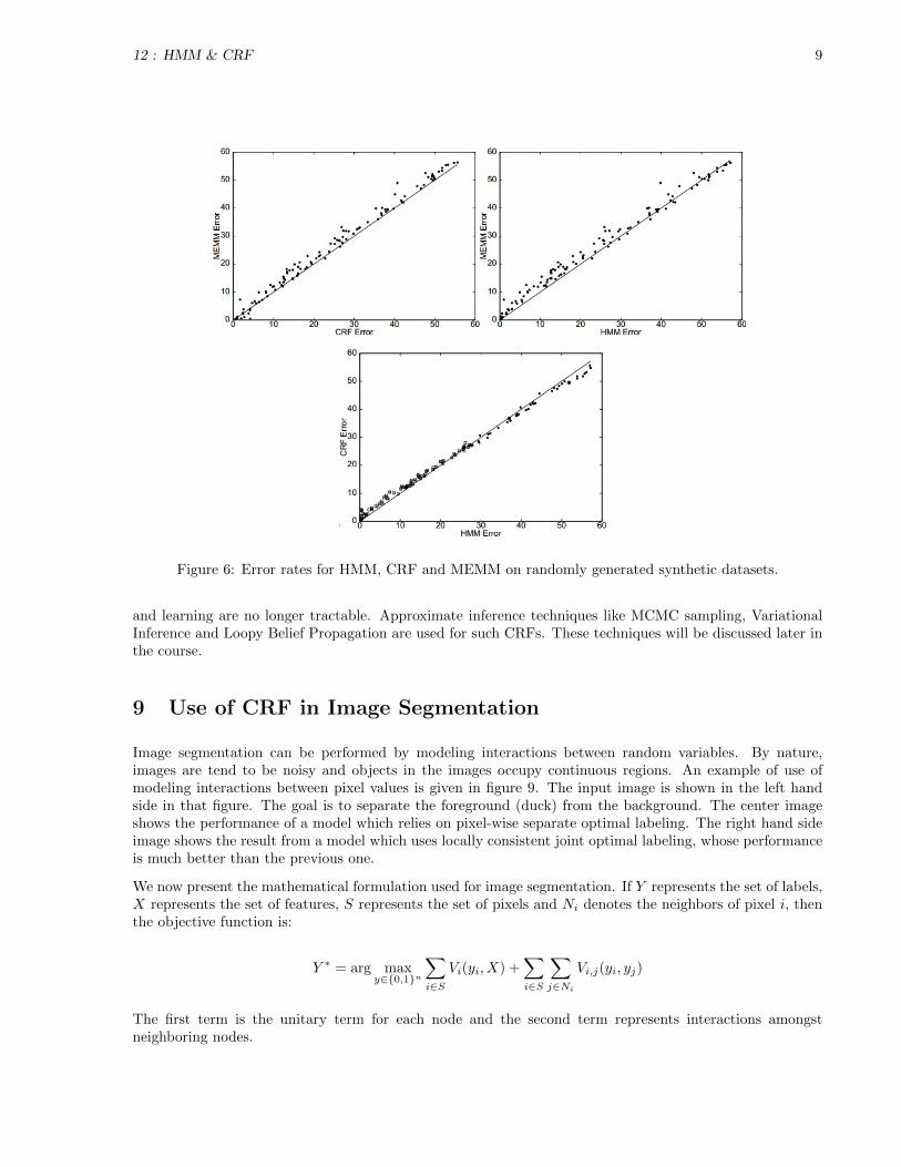
9 Use of CRF in Image Segmentation

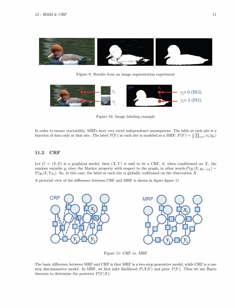
Image segmentation can be performed by modeling interactions between random variables. By nature,images are tend to be noisy and objects in the images occupy continuous regions. An example of use ofmodeling interactions between pixel values is given in figure 9. The input image is shown in the left handside in that figure. The goal is to separate the foreground (duck) from the background. The center imageshows the performance of a model which relies on pixel-wise separate optimal labeling. The right hand sideimage shows the result from a model which uses locally consistent joint optimal labeling, whose performanceis much better than the previous one.

We now present the mathematical formulation used for image segmentation. If Y represents the set of labels,X represents the set of features, S represents the set of pixels and Ni denotes the neighbors of pixel i, thenthe objective function is:

Y ∗ = arg maxy∈{0,1}n

∑i∈S

Vi(yi, X) +∑i∈S

∑j∈Ni

Vi,j(yi, yj)

The first term is the unitary term for each node and the second term represents interactions amongstneighboring nodes.

10 12 : HMM & CRF

Figure 7: Per-word error rates for parts of speech tagging experiment.

Figure 8: Grid CRF.

10 Image Labeling Example

Images can be represented by 4-connected 2D grid. Suppose X = {xi}i∈S represents observed data ofan image. Here xi represents data at the i-th site (pixel or block) of the image set S. Also suppose thatY = {yi}i∈S represents hidden labels at the i-th site, yi ∈ {1, ..., L}. Figure 10 gives a pictorial representationof X,Y and S. Then the objective is to maximize the conditional probability Y ∗ = arg maxY P (Y |X)

11 Difference Between MRF(Markov Random Field) and CRF

11.1 MRF

Y = {yi}i∈S is called MRF on the set S , with respect to neighborhood system N , iff for all i ∈ S,P (yi|yS−{i}) = P (yi|yNi).

In this case, the posterior probability is

P (Y |X) =P (X,Y )

P (X)∝ P (X|Y )P (Y ) =

∏i∈S

P (xi|yi).P (Y )

12 : HMM & CRF 11

Figure 9: Results from an image segmentation experiment

Figure 10: Image labeling example

In order to ensure tractability, MRFs have very strict independence assumptions. The lable at each site is afunction of data only at that site. The label P (Y ) at each site is modeled as a MRF: P (Y ) = 1

Z

∏c∈C ψc(yc)

11.2 CRF

Let G = (S,E) is a graphical model, then (X,Y ) is said to be a CRF, if, when conditioned on X, therandom variable yi obey the Markov property with respect to the graph, in other words:P (yi|X, yS−{i}) =P (yi|X,YNi). So, in this case, the label at each site is globally coditioned on the observation X.

A pictorial view of the difference between CRF and MRF is shown in figure figure 11

Figure 11: CRF vs. MRF

The basic difference between MRF and CRF is that MRF is a two-step generative model, while CRF is a onestep discriminative model. In MRF, we first infer likelihood P (X|Y ) and prior P (Y ). Then we use Bayestheorem to determine the posterior P (Y |X):

12 12 : HMM & CRF

P (Y |X) =P (X,Y )

P (X)∝ P (X|Y )P (Y ) =

∏i∈S

P (xi|yi).1

Z

∏c∈C

ψc(yc)

On the other hand, CRF is a one step discriminative model where the posterior P (Y |X) is infered directlyfrom data.

Popular formulation of MRF is:

P (Y |X) =1

Zexp(

∑i∈S

log p(xi|yi) +∑i∈S

∑j∈Ni

V2(yi, yj))

The assumption here is that of a Potts model for P (Y ) with only pairwise potential.

On the other hand, popular formulation for CRF is:

P (Y |X) =1

Zexp(−

∑i∈S

V1(yi|X) +∑i∈S

∑j∈Ni

V2(yi, yj |X))

Here only pairwise clique potentials is used.

12 Example of CRF-DRF

Discriminative Random Fields (DRF) is a special type of CRF where the unary and pairwise potentials aredesigned using local discriminative classifiers. In this case, the posterior probability is

P (Y |X) =1

Zexp(

∑i∈S

(A(yi, X) +∑i∈S

∑j∈Ni

Iij(yi, yj , X))

The posterior probability can be partitioned into an Association potential and an Interaction potential. TheAssociation potential is a local discriminative model for site i which is modeled using logistic link with GLM:

Ai(yi, X) = logP (yi|fi(X))

P (yi = 1|fi(X)) =1

1 + exp(−(wT fi(X))= σ(wT fi(X))

The Interaction potential is a measure of how likely site i and j have the same label given X:

Iij(yi, yj , X) = kyiyj + (1− k)(2σ(yiyjµij(X))− 1))

The first part in the above equation is a data dependent smoothing term and the second part is pairwiselogistic function.

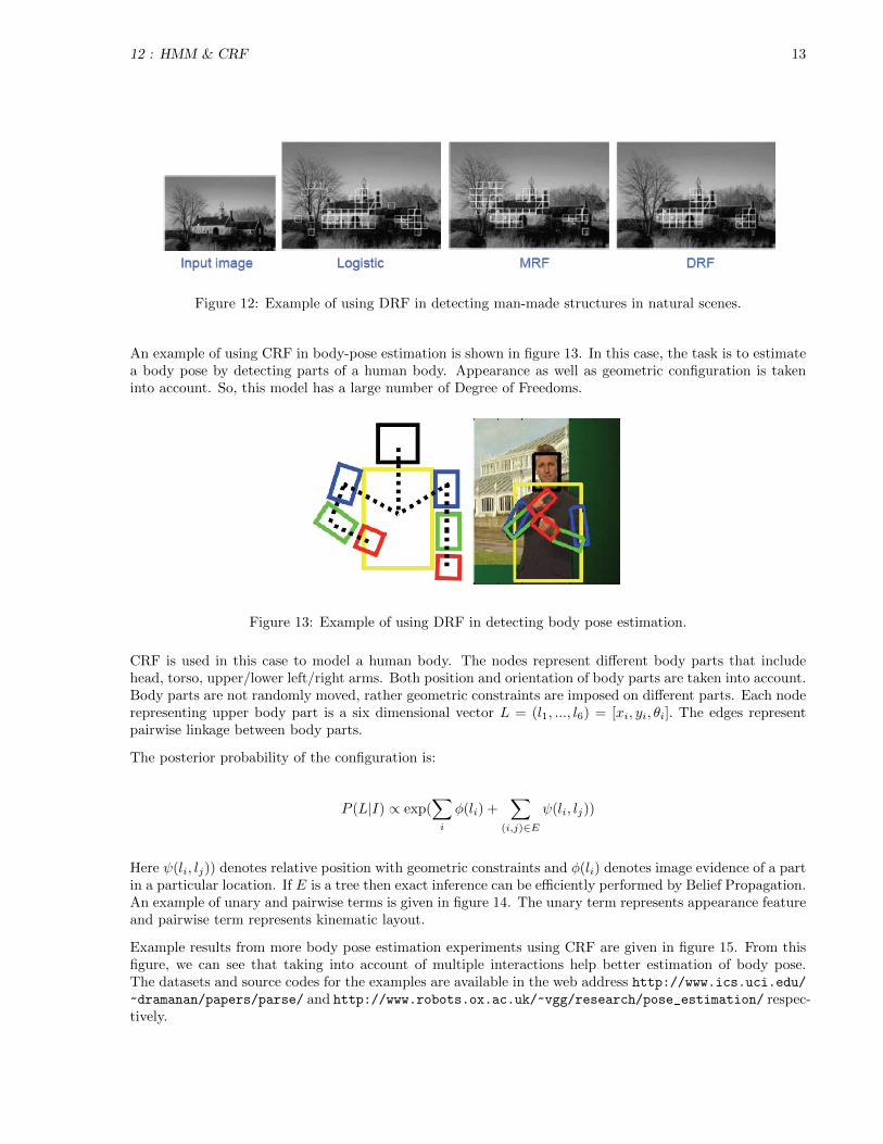
The result of using DRF and two other similar approaches (Logistic Regression and MRF in this case) indetecting man-made structure in local scenes is shown in figure 12. For this experiment, each image isdivided into non-overlapping 16x16 tile blocks.

The logistic regression does not assume any smoothness in the labels. In the case of MRF, false positivesare smoothed out. But lack of neighborhood interaction of the data hurts its performance. Among the threeapproaches, DRF shows the best performance.

12 : HMM & CRF 13

Figure 12: Example of using DRF in detecting man-made structures in natural scenes.

An example of using CRF in body-pose estimation is shown in figure 13. In this case, the task is to estimatea body pose by detecting parts of a human body. Appearance as well as geometric configuration is takeninto account. So, this model has a large number of Degree of Freedoms.

Figure 13: Example of using DRF in detecting body pose estimation.

CRF is used in this case to model a human body. The nodes represent different body parts that includehead, torso, upper/lower left/right arms. Both position and orientation of body parts are taken into account.Body parts are not randomly moved, rather geometric constraints are imposed on different parts. Each noderepresenting upper body part is a six dimensional vector L = (l1, ..., l6) = [xi, yi, θi]. The edges representpairwise linkage between body parts.

The posterior probability of the configuration is:

P (L|I) ∝ exp(∑i

φ(li) +∑

(i,j)∈E

ψ(li, lj))

Here ψ(li, lj)) denotes relative position with geometric constraints and φ(li) denotes image evidence of a partin a particular location. If E is a tree then exact inference can be efficiently performed by Belief Propagation.An example of unary and pairwise terms is given in figure 14. The unary term represents appearance featureand pairwise term represents kinematic layout.

Example results from more body pose estimation experiments using CRF are given in figure 15. From thisfigure, we can see that taking into account of multiple interactions help better estimation of body pose.The datasets and source codes for the examples are available in the web address http://www.ics.uci.edu/

~dramanan/papers/parse/ and http://www.robots.ox.ac.uk/~vgg/research/pose_estimation/ respec-tively.

14 12 : HMM & CRF

Figure 14: Example of (A)unary and (B)pariwise terms in body pose estimation example.

Figure 15: Example results from body pose estimation experiments using CRF.

13 Conclusions

The take home messages from today’s lecture are following:

• CRFs are partially directed discriminative model.

• CRFs overcome the label bias problem of MEMMs by using a global normalizer.

• For 1-D chain CRF, the inference problem is exact and can be solved using techniques such as maxproduct algorithm or Viterbi decoding.

• For chain CRFs, learning is also exact and globally optimum parameters can be learned. Sum productor forward-backward algorithm can be used for learning purpose.

• CRFs involving arbitrary graph structure other than chain or tree are intractable in general. For theseCRFs, inference and learning require approximation techniques such as MCMC sampling, Variationalmethods or Loopy belief propagation.