Embed Size (px)
Citation preview
12INFINITE SEQUENCES AND SERIESINFINITE SEQUENCES AND SERIES
In section 12.9, we were able to
find power series representations for
a certain restricted class of functions.
INFINITE SEQUENCES AND SERIES

Here, we investigate more general
problems.
Which functions have power series representations?
How can we find such representations?
INFINITE SEQUENCES AND SERIES
12.10Taylor and Maclaurin Series
INFINITE SEQUENCES AND SERIES
In this section, we will learn:
How to find the Taylor and Maclaurin Series of a function
and to multiply and divide a power series.
TAYLOR & MACLAURIN SERIES
We start by supposing that f is any function
that can be represented by a power series
20 1 2
3 43 4
( ) ( ) ( )
( ) ( ) ... | |
f x c c x a c x a
c x a c x a x a R
Equation 1
TAYLOR & MACLAURIN SERIES
Let’s try to determine what the
coefficients cn must be in terms of f.
To begin, notice that, if we put x = a in Equation 1, then all terms after the first one are 0 and we get:
f(a) = c0
TAYLOR & MACLAURIN SERIES
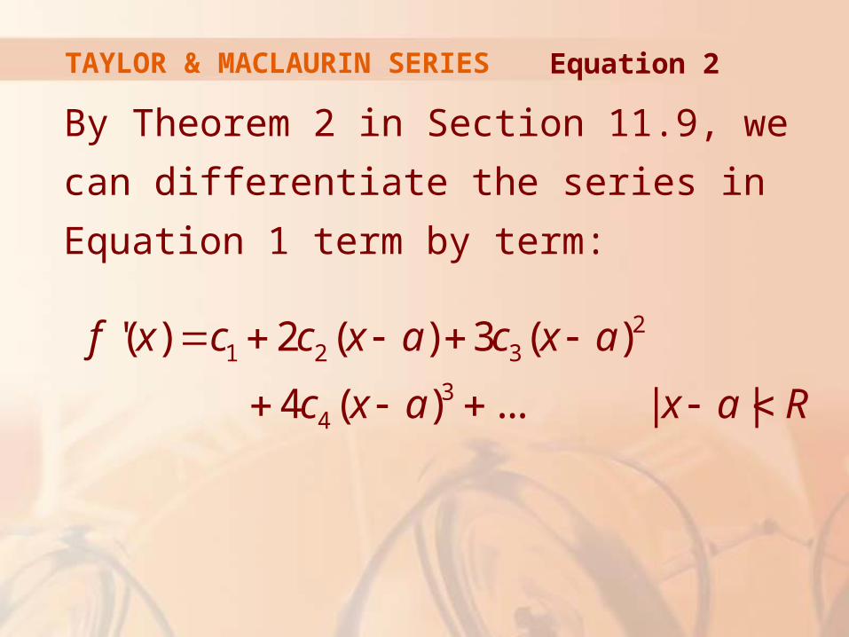
By Theorem 2 in Section 11.9, we can
differentiate the series in Equation 1 term by
term:
21 2 3
34
'( ) 2 ( ) 3 ( )
4 ( ) ... | |
f x c c x a c x a
c x a x a R
Equation 2
TAYLOR & MACLAURIN SERIES
Substitution of x = a in Equation 2
gives:
f’(a) = c1
TAYLOR & MACLAURIN SERIES
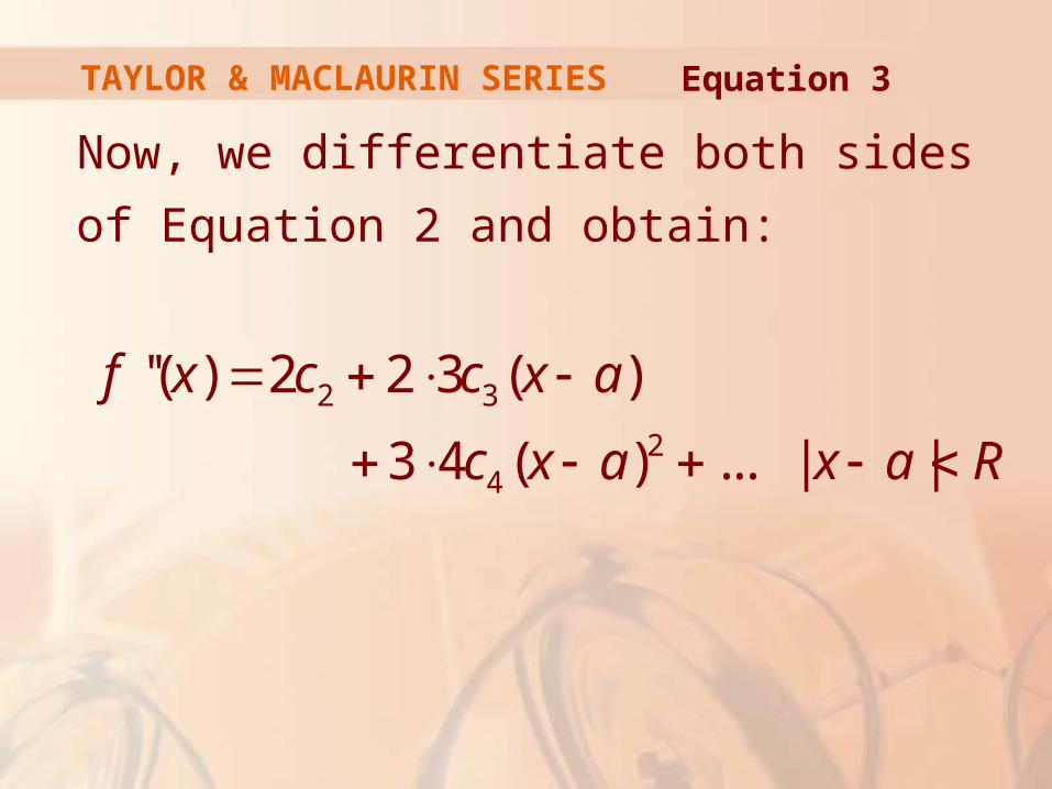
Now, we differentiate both sides of Equation 2
and obtain:
2 3
24
''( ) 2 2 3 ( )
3 4 ( ) ... | |
f x c c x a
c x a x a R
Equation 3
TAYLOR & MACLAURIN SERIES
Again, we put x = a in Equation 3.
The result is:
f’’(a) = 2c2

TAYLOR & MACLAURIN SERIES
Let’s apply the procedure
one more time.
TAYLOR & MACLAURIN SERIES
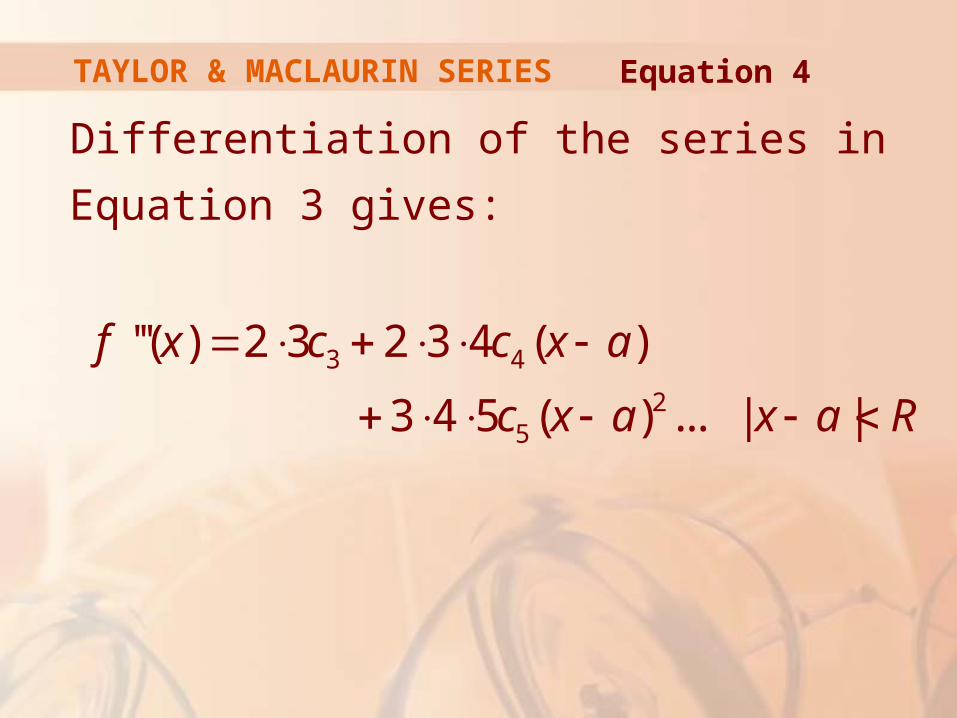
Differentiation of the series in Equation 3
gives:
3 4
25
'''( ) 2 3 2 3 4 ( )
3 4 5 ( ) ... | |
f x c c x a
c x a x a R
Equation 4
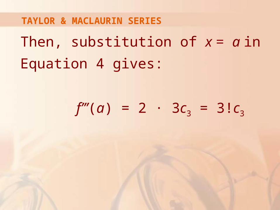
TAYLOR & MACLAURIN SERIES
Then, substitution of x = a in Equation 4
gives:
f’’’(a) = 2 · 3c3 = 3!c3
TAYLOR & MACLAURIN SERIES
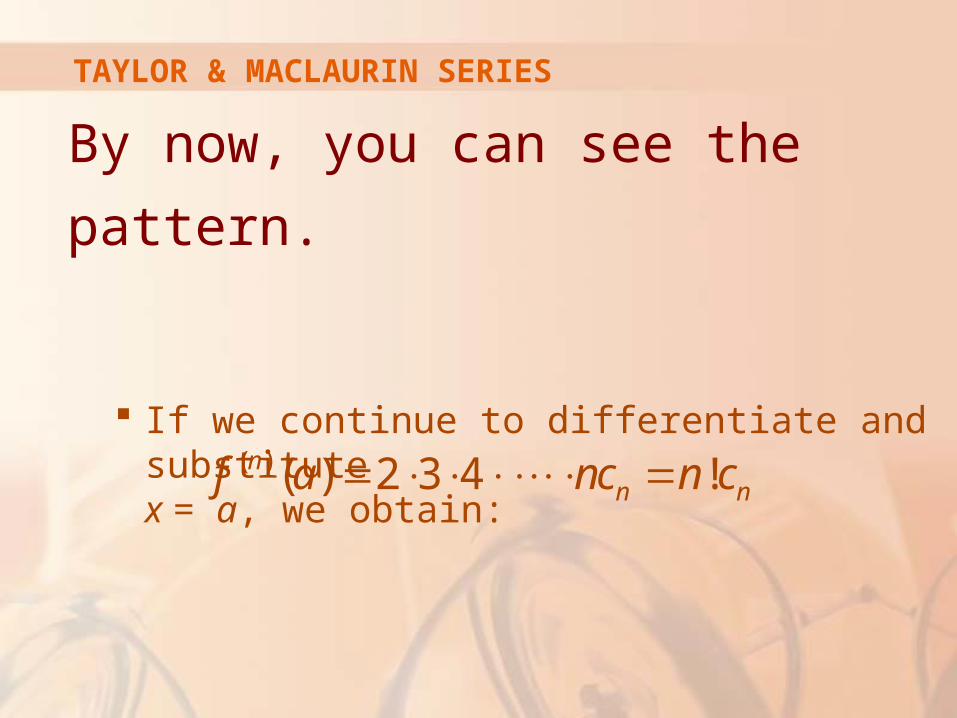
By now, you can see the pattern.
If we continue to differentiate and substitute x = a, we obtain:
( ) ( ) 2 3 4 !nn nf a nc n c
TAYLOR & MACLAURIN SERIES
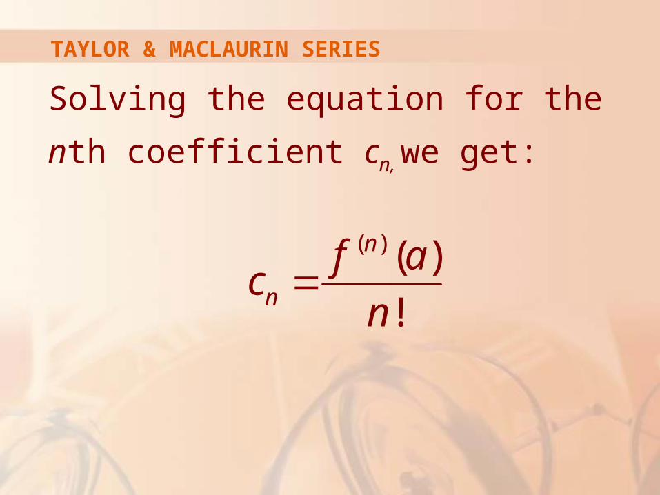
Solving the equation for the nth
coefficient cn, we get:
( ) ( )
!
n
n
f ac
n
TAYLOR & MACLAURIN SERIES
The formula remains valid even for n = 0
if we adopt the conventions that 0! = 1
and f (0) = (f).
Thus, we have proved the following theorem.
TAYLOR & MACLAURIN SERIES
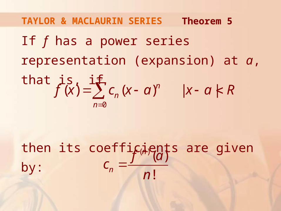
If f has a power series representation
(expansion) at a, that is, if
then its coefficients are given by:
Theorem 5
0
( ) ( ) | |nn
n
f x c x a x a R
( ) ( )
!
n
n
f ac
n
TAYLOR & MACLAURIN SERIES
Substituting this formula for cn back into
the series, we see that if f has a power series
expansion at a, then it must be of the following
form.
Equation 6
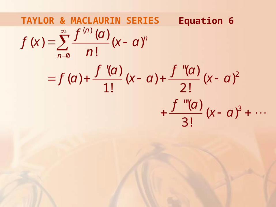
TAYLOR & MACLAURIN SERIES Equation 6( )
0
2
3
( )( ) ( )
!
'( ) ''( )( ) ( ) ( )
1! 2!'''( )
( )3!
nn
n
f af x x a
n
f a f af a x a x a
f ax a
TAYLOR SERIES
The series in Equation 6 is called
the Taylor series of the function f at a
(or about a or centered at a).
TAYLOR SERIES
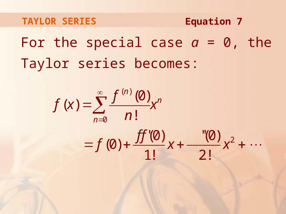
For the special case a = 0, the Taylor series
becomes:
( )
0
2
(0)( )
!
'(0) ''(0)(0)
1! 2!
nn
n
ff x x
n
f ff x x
Equation 7
MACLAURIN SERIES
This case arises frequently
enough that it is given the special
name Maclaurin series.
Equation 7
TAYLOR & MACLAURIN SERIES
The Taylor series is named after the English
mathematician Brook Taylor (1685–1731).
The Maclaurin series is named for the Scottish
mathematician Colin Maclaurin (1698–1746).
This is despite the fact that the Maclaurin series is really just a special case of the Taylor series.
MACLAURIN SERIES
Maclaurin series are named after Colin
Maclaurin because he popularized them
in his calculus textbook Treatise of Fluxions
published in 1742.
TAYLOR & MACLAURIN SERIES
We have shown that if, f can be represented
as a power series about a, then f is equal to
the sum of its Taylor series.
However, there exist functions that are not equal to the sum of their Taylor series.
An example is given in Exercise 70.
Note
TAYLOR & MACLAURIN SERIES
Find the Maclaurin series
of the function f(x) = ex and
its radius of convergence.
Example 1
TAYLOR & MACLAURIN SERIES
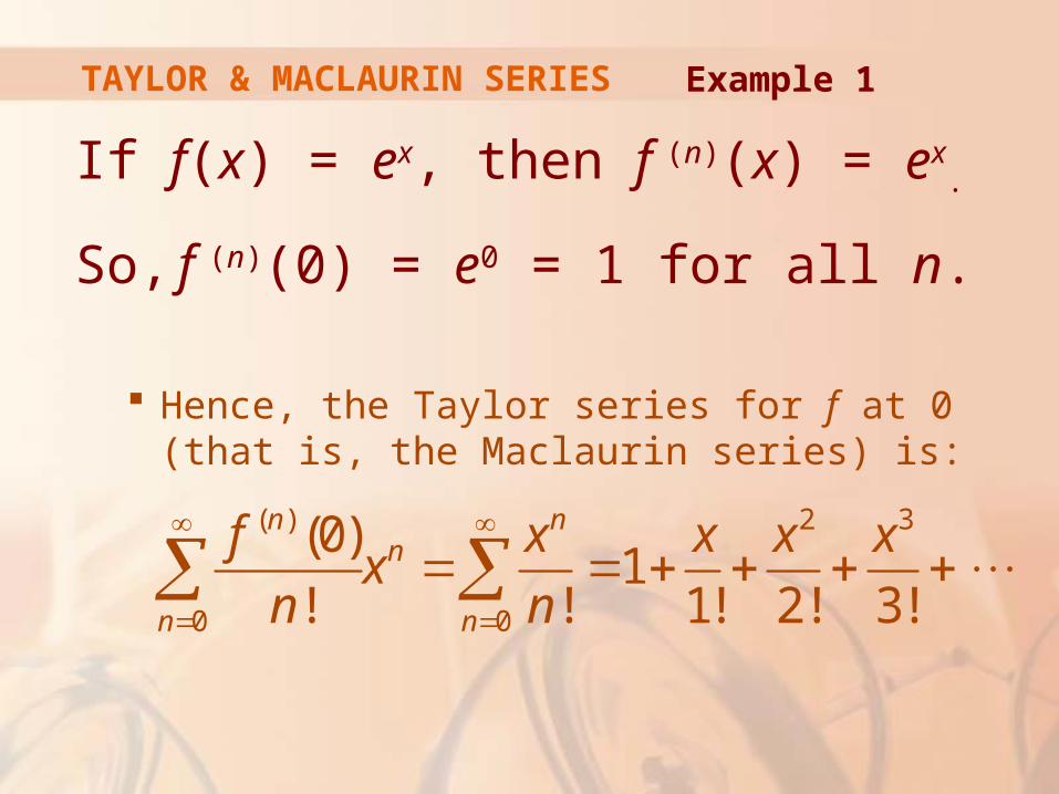
If f(x) = ex, then f (n)(x) = ex.
So, f (n)(0) = e0 = 1 for all n.
Hence, the Taylor series for f at 0 (that is, the Maclaurin series) is:
Example 1
( ) 2 3
0 0
(0)1
! ! 1! 2! 3!
n nn
n n
f x x x xx
n n
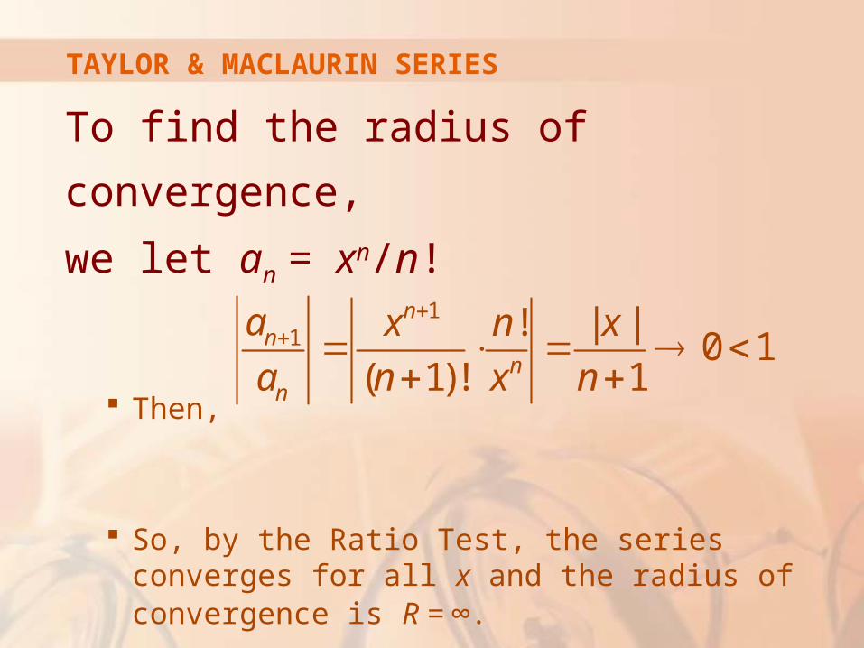
TAYLOR & MACLAURIN SERIES
To find the radius of convergence,
we let an = xn/n!
Then,
So, by the Ratio Test, the series converges for all x and the radius of convergence is R = ∞.
11 ! | |
0 1( 1)! 1
nn
nn
a x n x
a n x n
TAYLOR & MACLAURIN SERIES
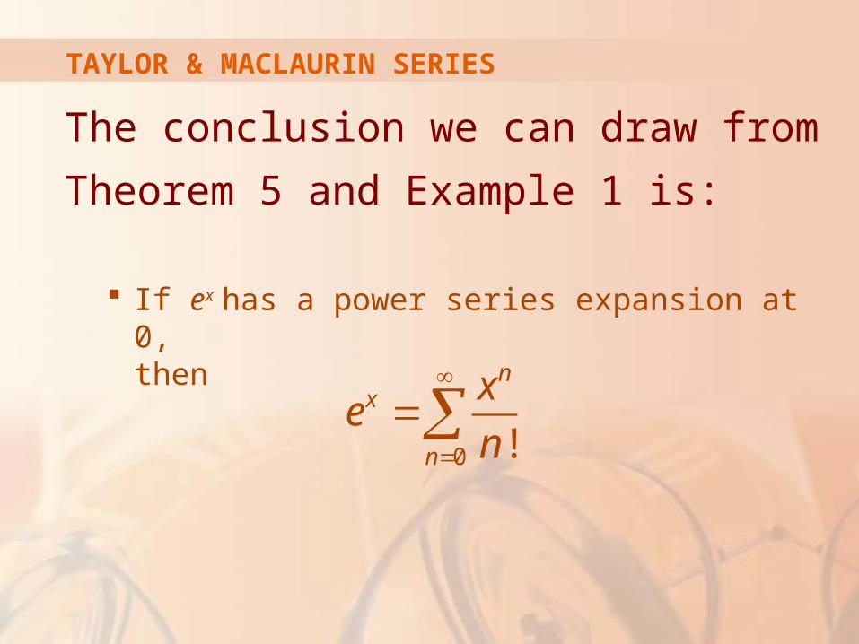
The conclusion we can draw from
Theorem 5 and Example 1 is:
If ex has a power series expansion at 0, then
0 !
nx
n
xe
n
TAYLOR & MACLAURIN SERIES
So, how can we determine
whether ex does have a power
series representation?
TAYLOR & MACLAURIN SERIES
Let’s investigate the more general
question:
Under what circumstances is a function equal to the sum of its Taylor series?
TAYLOR & MACLAURIN SERIES
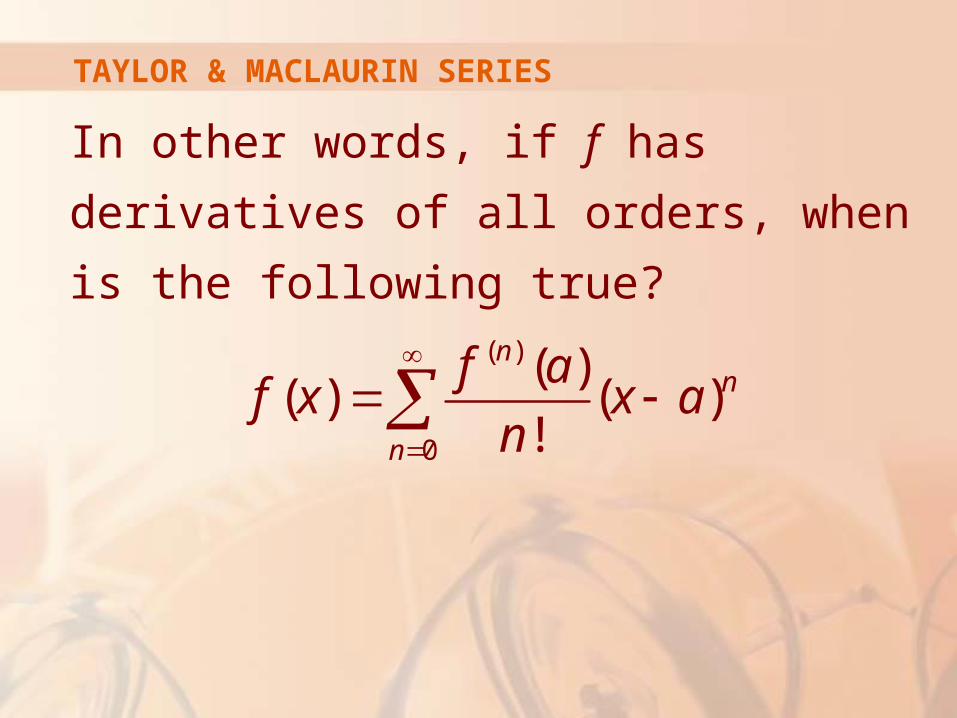
In other words, if f has derivatives of all
orders, when is the following true?
( )
0
( )( ) ( )
!
nn
n
f af x x a
n
TAYLOR & MACLAURIN SERIES
As with any convergent series,
this means that f(x) is the limit of
the sequence of partial sums.
TAYLOR & MACLAURIN SERIES
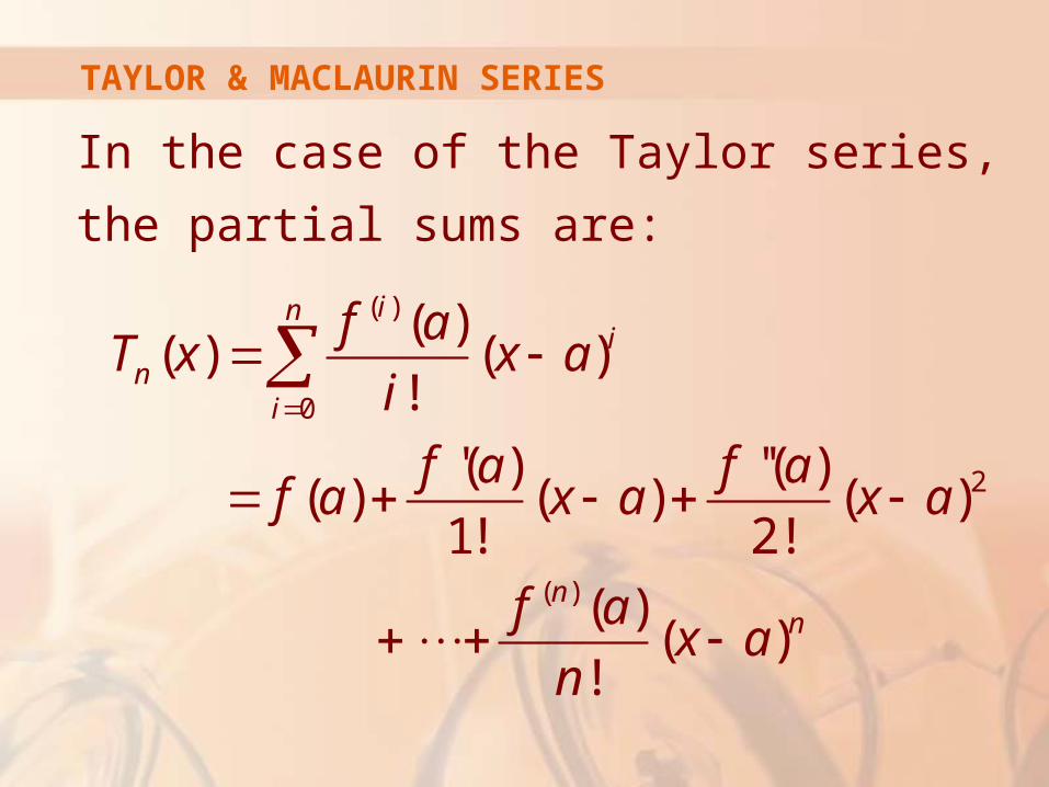
In the case of the Taylor series, the partial
sums are:
( )
0
2
( )
( )( ) ( )
!
'( ) ''( )( ) ( ) ( )
1! 2!
( )( )
!
ini
ni
nn
f aT x x a
i
f a f af a x a x a
f ax a
n
nTH-DEGREE TAYLOR POLYNOMIAL OF f AT a
Notice that Tn is a polynomial
of degree n called the nth-degree Taylor
polynomial of f at a.
TAYLOR & MACLAURIN SERIES
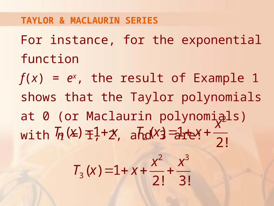
For instance, for the exponential function
f(x) = ex, the result of Example 1 shows that
the Taylor polynomials at 0 (or Maclaurin
polynomials) with n = 1, 2, and 3 are:
2
1 2
2 3
3
( ) 1 ( ) 12!
( ) 12! 3!
xT x x T x x
x xT x x
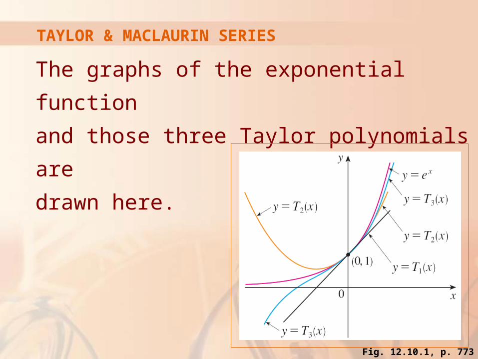
TAYLOR & MACLAURIN SERIES
The graphs of the exponential function
and those three Taylor polynomials are
drawn here.
Fig. 12.10.1, p. 773
TAYLOR & MACLAURIN SERIES
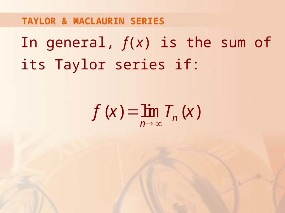
In general, f(x) is the sum of its Taylor
series if:
( ) lim ( )nn
f x T x
REMAINDER OF TAYLOR SERIES
If we let Rn(x) = f(x) – Tn(x)
so that f(x) = Tn(x) + Rn(x)
then Rn(x) is called the remainder of
the Taylor series.
TAYLOR & MACLAURIN SERIES
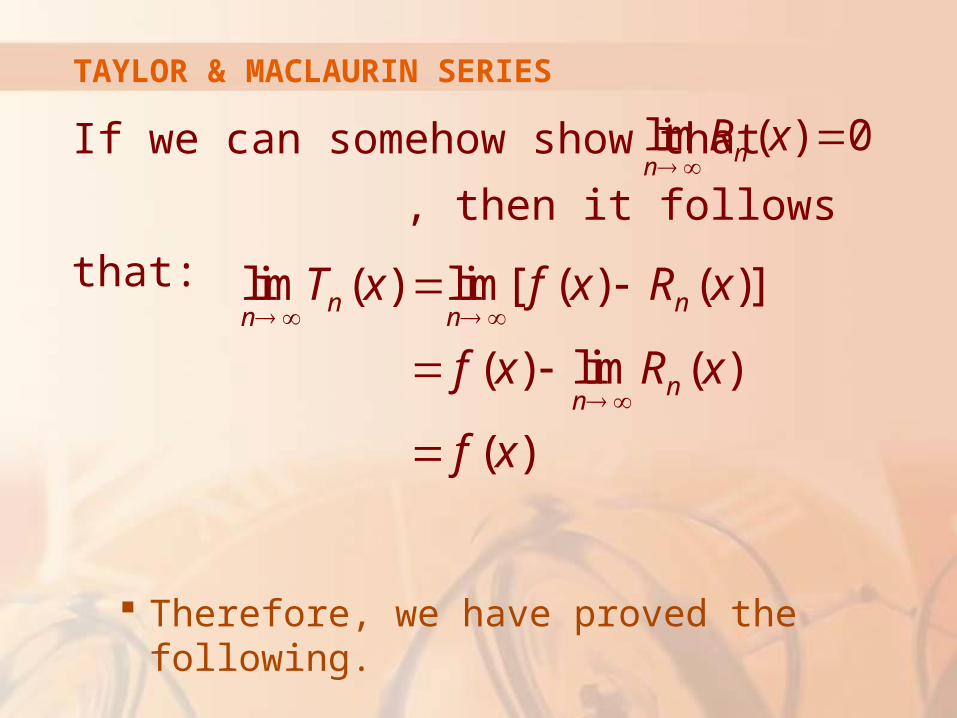
If we can somehow show that ,
then it follows that:
Therefore, we have proved the following.
lim ( ) 0nnR x
lim ( ) lim[ ( ) ( )]
( ) lim ( )
( )
n nn n
nn
T x f x R x
f x R x
f x
TAYLOR & MACLAURIN SERIES
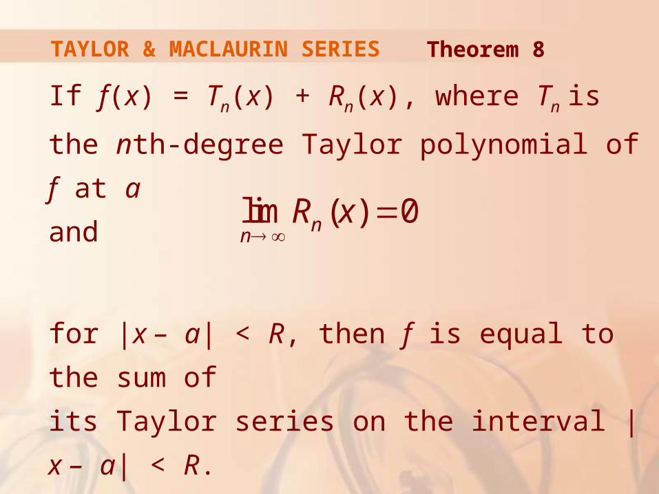
If f(x) = Tn(x) + Rn(x), where Tn is
the nth-degree Taylor polynomial of f at a
and
for |x – a| < R, then f is equal to the sum of
its Taylor series on the interval |x – a| < R.
Theorem 8
lim ( ) 0nnR x
TAYLOR & MACLAURIN SERIES
In trying to show that
for a specific function f, we usually use
the following fact.
lim ( ) 0nnR x
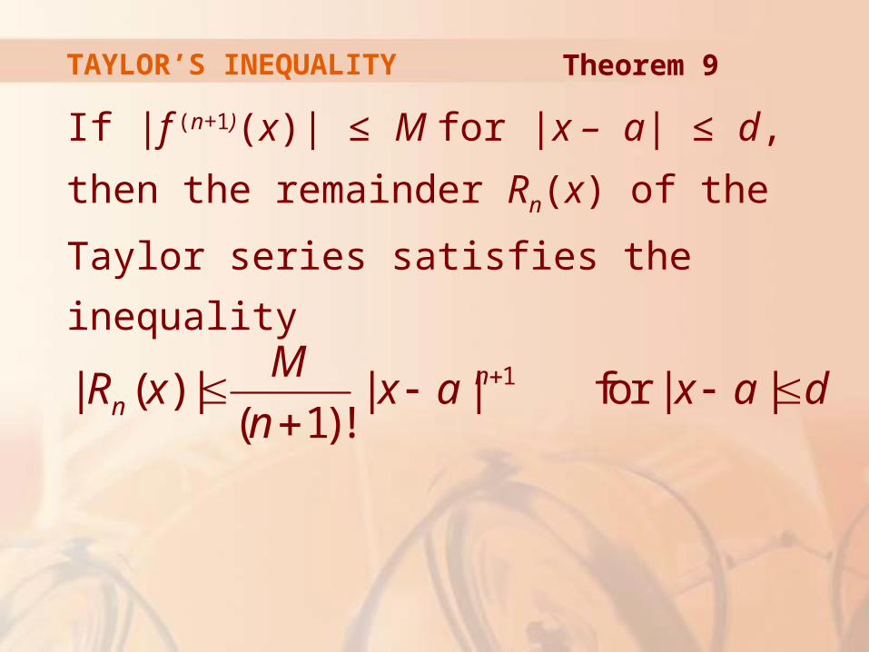
TAYLOR’S INEQUALITY
If |f (n+1)(x)| ≤ M for |x – a| ≤ d,
then the remainder Rn(x) of the Taylor series
satisfies the inequality
Theorem 9
1| ( ) | | | for | |( 1)!
nn
MR x x a x a d
n
TAYLOR’S INEQUALITY
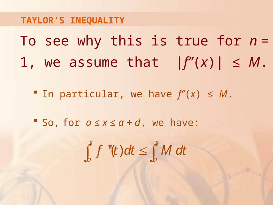
To see why this is true for n = 1, we
assume that |f’’(x)| ≤ M.
In particular, we have f’’(x) ≤ M.
So, for a ≤ x ≤ a + d, we have:
''( )x x
a af t dt M dt
TAYLOR’S INEQUALITY
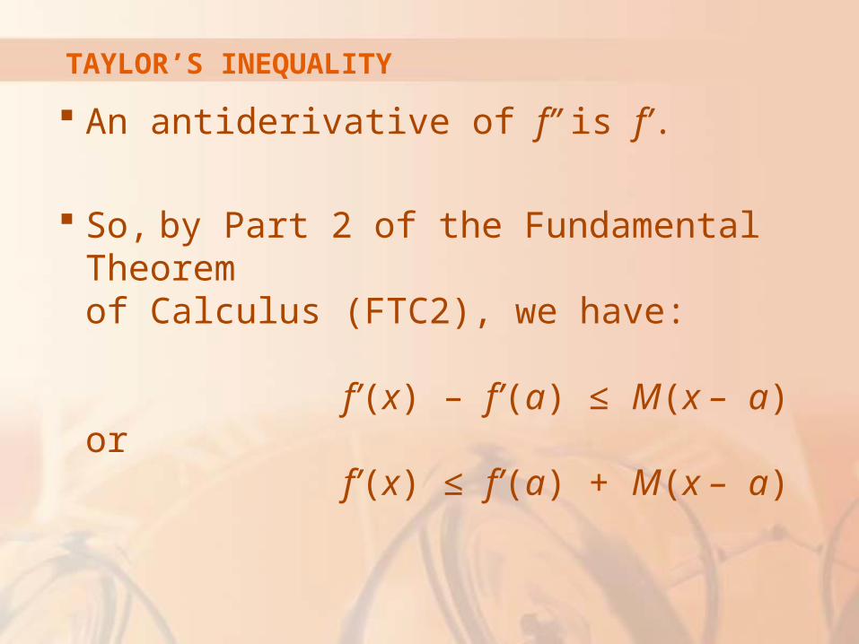
An antiderivative of f’’ is f’.
So, by Part 2 of the Fundamental Theorem of Calculus (FTC2), we have:
f’(x) – f’(a) ≤ M(x – a) or
f’(x) ≤ f’(a) + M(x – a)
TAYLOR’S INEQUALITY
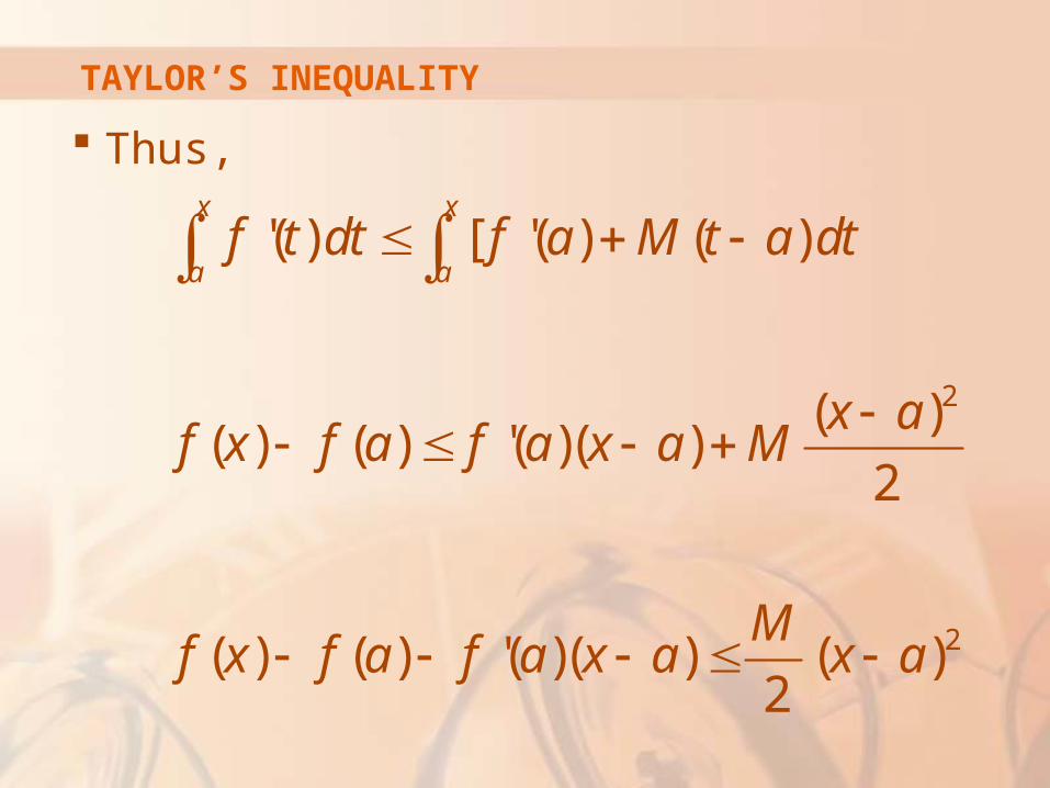
Thus,
2
2
'( ) [ '( ) ( )
( )( ) ( ) '( )( )
2
( ) ( ) '( )( ) ( )2
x x
a af t dt f a M t a dt
x af x f a f a x a M
Mf x f a f a x a x a
TAYLOR’S INEQUALITY
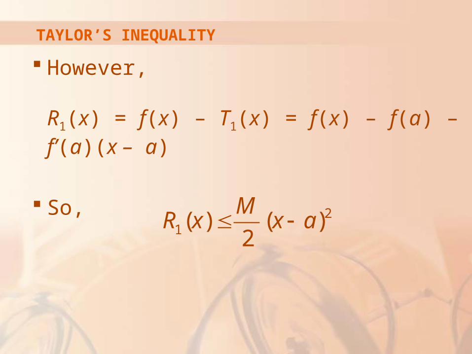
However,
R1(x) = f(x) – T1(x) = f(x) – f(a) – f’(a)(x – a)
So,2
1( ) ( )2
MR x x a
TAYLOR’S INEQUALITY
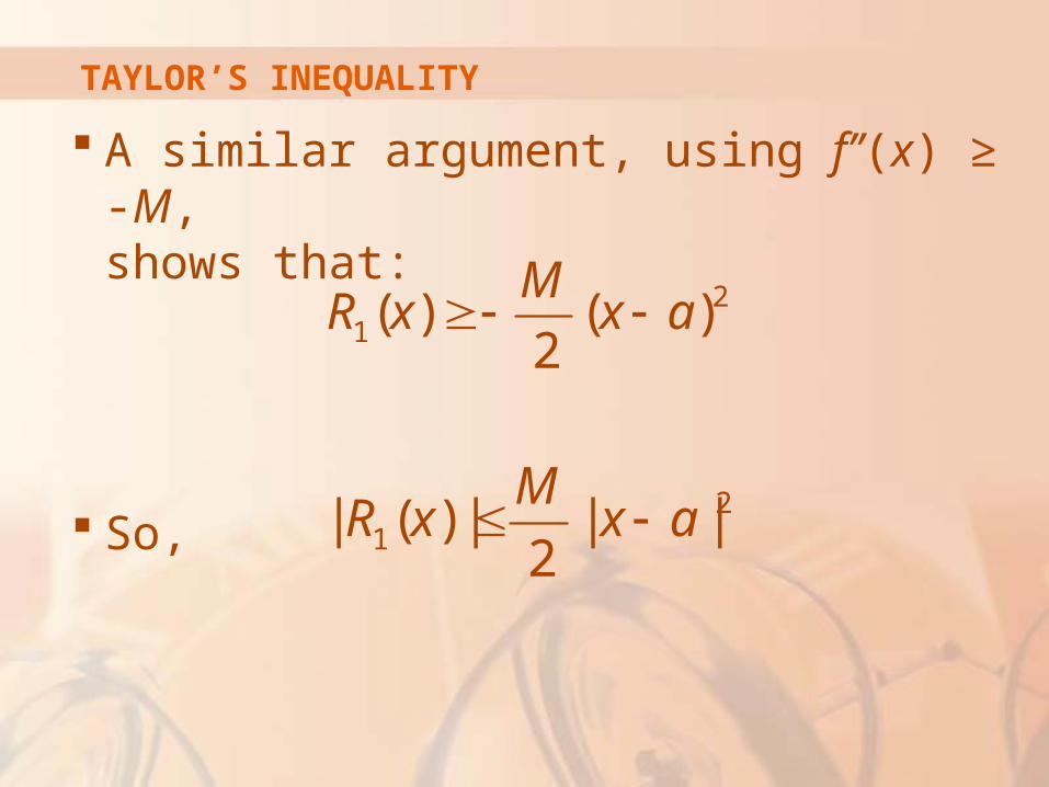
A similar argument, using f’’(x) ≥ -M, shows that:
So,
21( ) ( )
2
MR x x a
21| ( ) | | |
2
MR x x a
TAYLOR’S INEQUALITY
We have assumed that x > a.
However, similar calculations show that this inequality is also true for x < a.
TAYLOR’S INEQUALITY
This proves Taylor’s Inequality for
the case where n = 1.
The result for any n is proved in a similar way by integrating n + 1 times.
See Exercise 69 for the case n = 2
TAYLOR’S INEQUALITY
In Section 11.11, we will explore the use of
Taylor’s Inequality in approximating functions.
Our immediate use of it is in conjunction with
Theorem 8.
Note
TAYLOR’S INEQUALITY
In applying Theorems 8 and 9,
it is often helpful to make use of
the following fact.
TAYLOR’S INEQUALITY
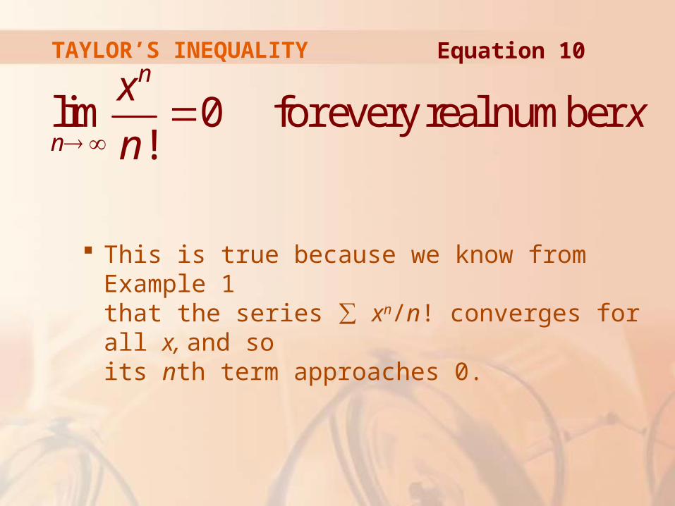
This is true because we know from Example 1 that the series ∑ xn/n! converges for all x, and so its nth term approaches 0.
lim 0 for every real number!
n
n
xx
n
Equation 10
TAYLOR’S INEQUALITY
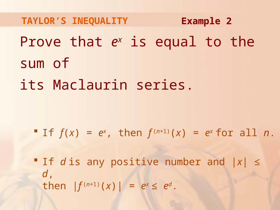
Prove that ex is equal to the sum of
its Maclaurin series.
If f(x) = ex, then f (n+1)(x) = ex for all n.
If d is any positive number and |x| ≤ d, then |f (n+1)(x)| = ex ≤ ed.
Example 2
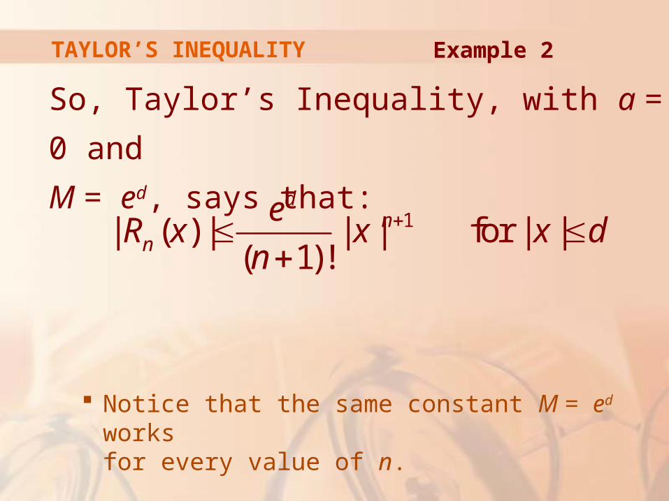
TAYLOR’S INEQUALITY
So, Taylor’s Inequality, with a = 0 and
M = ed, says that:
Notice that the same constant M = ed works for every value of n.
1| ( ) | | | for | |( 1)!
dn
n
eR x x x d
n
Example 2
TAYLOR’S INEQUALITY
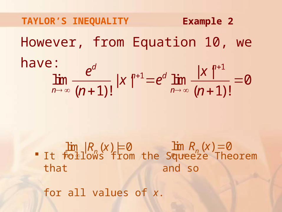
However, from Equation 10, we have:
It follows from the Squeeze Theorem that and so
for all values of x.
11 | |
lim | | lim 0( 1)! ( 1)!
d nn d
n n
e xx e
n n
lim ( ) 0nnR x
Example 2
lim | ( ) | 0nn
R x
TAYLOR’S INEQUALITY
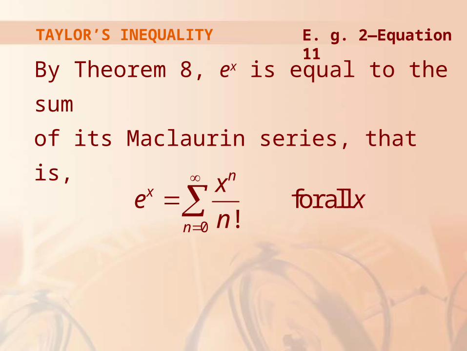
By Theorem 8, ex is equal to the sum
of its Maclaurin series, that is,
0
for all!
nx
n
xe x
n
E. g. 2—Equation 11
TAYLOR & MACLAURIN SERIES
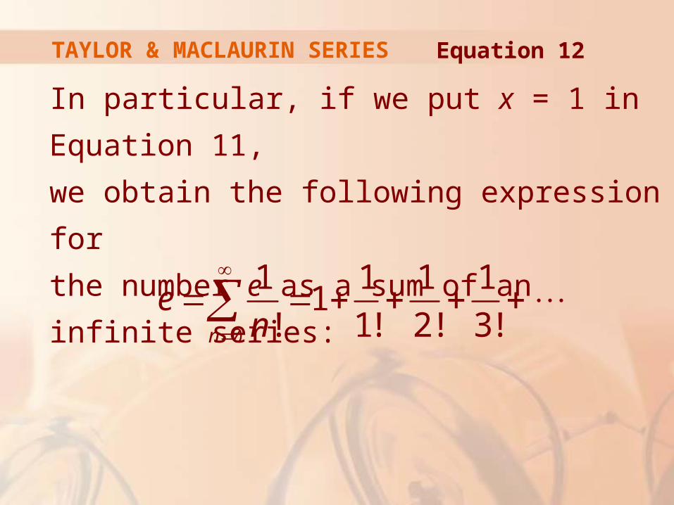
In particular, if we put x = 1 in Equation 11,
we obtain the following expression for
the number e as a sum of an infinite series:
0
1 1 1 11
! 1! 2! 3!n
en
Equation 12
TAYLOR & MACLAURIN SERIES
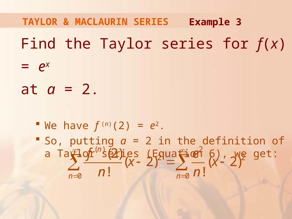
Find the Taylor series for f(x) = ex
at a = 2.
We have f (n)(2) = e2. So, putting a = 2 in the definition of a Taylor series
(Equation 6), we get:
Example 3
( ) 22 2
0 0
(2)( 2) ( 2)
! !
n
n n
f ex x
n n
TAYLOR & MACLAURIN SERIES
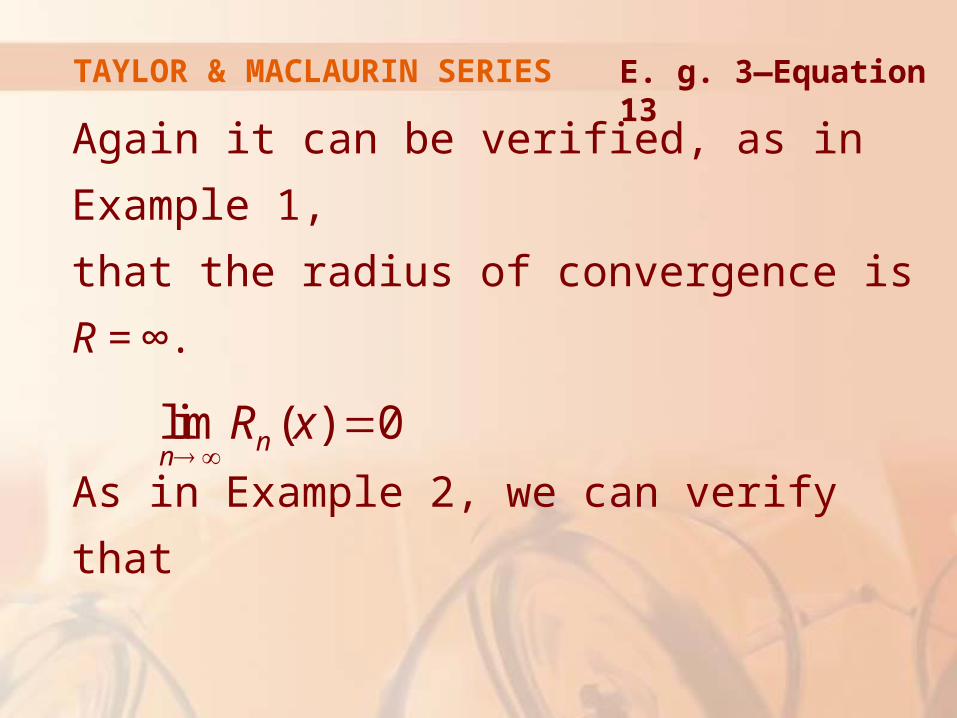
Again it can be verified, as in Example 1,
that the radius of convergence is R = ∞.
As in Example 2, we can verify
that lim ( ) 0nnR x
E. g. 3—Equation 13
TAYLOR & MACLAURIN SERIES
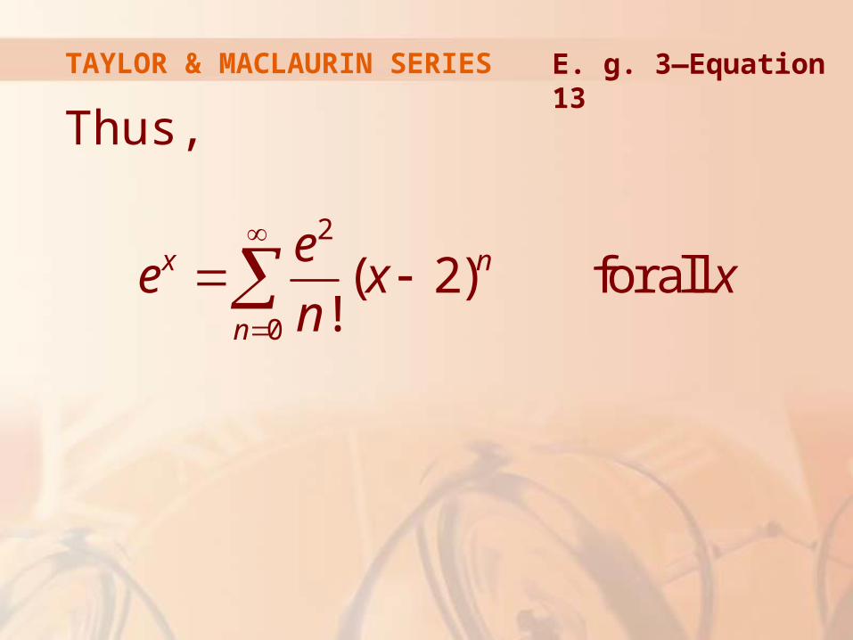
Thus,
2
0
( 2) for all!
x n
n
ee x x
n
E. g. 3—Equation 13
TAYLOR & MACLAURIN SERIES
We have two power series expansions for ex,
the Maclaurin series in Equation 11 and the
Taylor series in Equation 13.
The first is better if we are interested in values of x near 0.
The second is better if x is near 2.
TAYLOR & MACLAURIN SERIES
Find the Maclaurin series for sin x
and prove that it represents sin x
for all x.
Example 4
TAYLOR & MACLAURIN SERIES
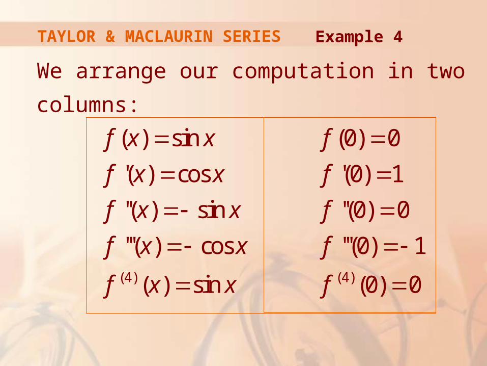
We arrange our computation in two columns:
(4) (4)
( ) sin (0) 0
'( ) cos '(0) 1
''( ) sin ''(0) 0
'''( ) cos '''(0) 1
( ) sin (0) 0
f x x f
f x x f
f x x f
f x x f
f x x f
Example 4
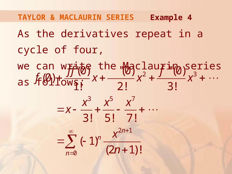
TAYLOR & MACLAURIN SERIES
As the derivatives repeat in a cycle of four,
we can write the Maclaurin series as follows:
2 3
3 5 7
2 1
0
'(0) ''(0) '''(0)(0)
1! 2! 3!
3! 5! 7!
( 1)(2 1)!
nn
n
f f ff x x x
x x xx
x
n
Example 4
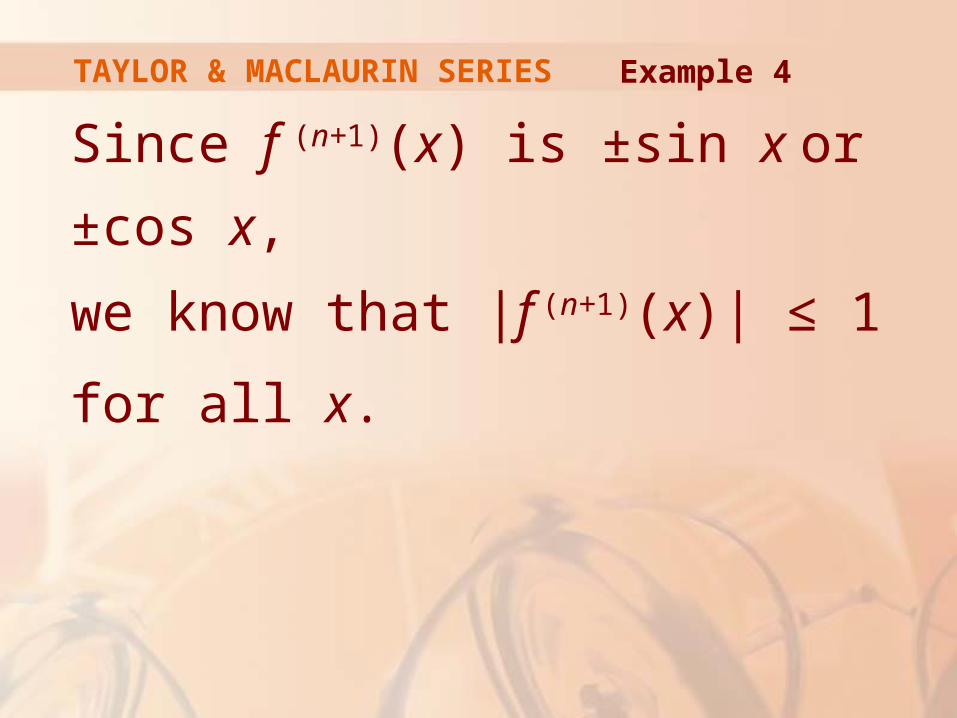
TAYLOR & MACLAURIN SERIES
Since f (n+1)(x) is ±sin x or ±cos x,
we know that |f (n+1)(x)| ≤ 1 for all x.
Example 4
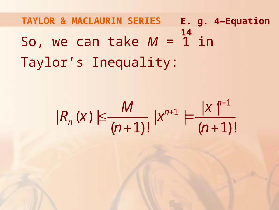
TAYLOR & MACLAURIN SERIES
So, we can take M = 1 in Taylor’s
Inequality:
11 | |
| ( ) | | |( 1)! ( 1)!
nn
n
M xR x x
n n
E. g. 4—Equation 14
TAYLOR & MACLAURIN SERIES
By Equation 10, the right side of that inequality
approaches 0 as n → ∞.
So, |Rn(x)| → 0 by the Squeeze Theorem.
It follows that Rn(x) → 0 as n → ∞.
So, sin x is equal to the sum of its Maclaurin series by Theorem 8.
Example 4
TAYLOR & MACLAURIN SERIES
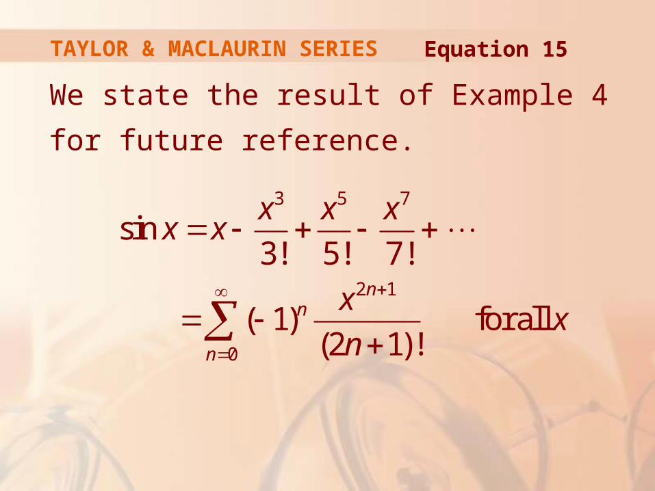
We state the result of Example 4 for future
reference.
3 5 7
2 1
0
sin3! 5! 7!
( 1) for all(2 1)!
nn
n
x x xx x
xx
n
Equation 15
TAYLOR & MACLAURIN SERIES
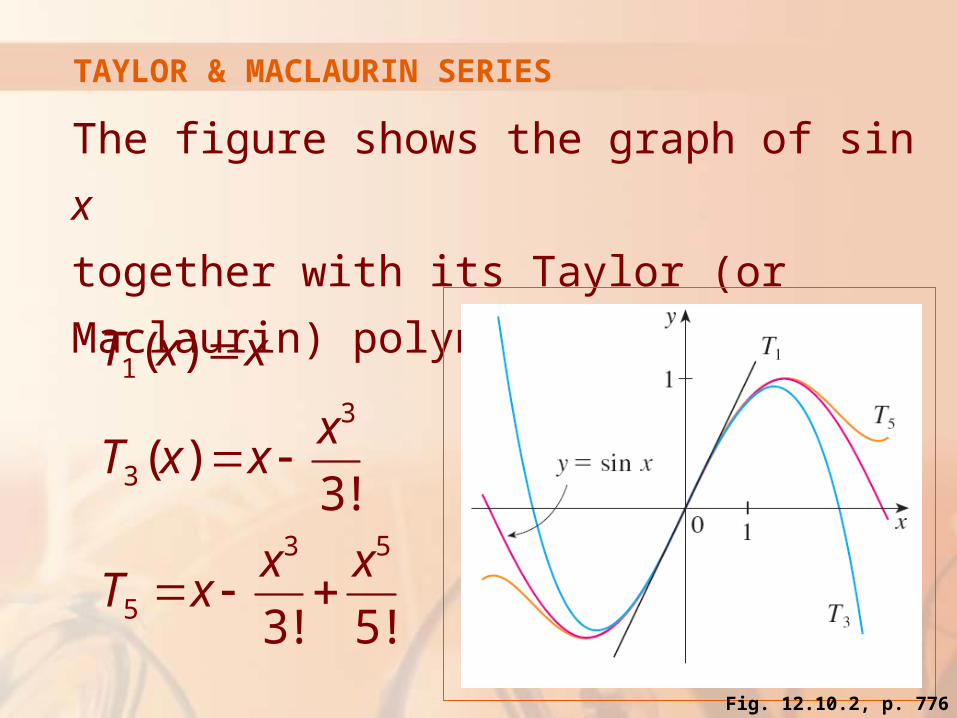
The figure shows the graph of sin x
together with its Taylor (or Maclaurin)
polynomials
1
3
3
3 5
5
( )
( )3!
3! 5!
T x x
xT x x
x xT x
Fig. 12.10.2, p. 776
TAYLOR & MACLAURIN SERIES
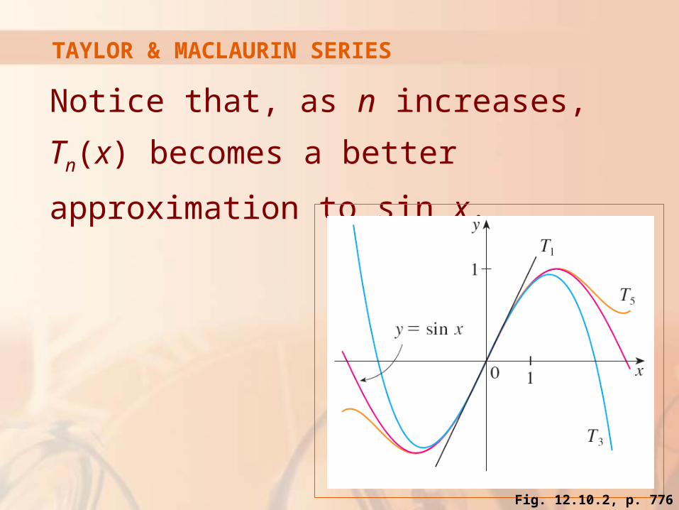
Notice that, as n increases, Tn(x) becomes
a better approximation to sin x.
Fig. 12.10.2, p. 776
TAYLOR & MACLAURIN SERIES
Find the Maclaurin series for cos x.
We could proceed directly as in Example 4.
However, it’s easier to differentiate the Maclaurin series for sin x given by Equation 15, as follows.
Example 5
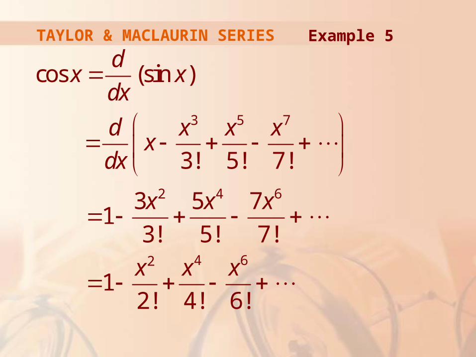
TAYLOR & MACLAURIN SERIES Example 5
3 5 7
2 4 6
4 62
cos (sin )
3! 5! 7!
3 5 71
3! 5! 7!
12! 4! 6!
dx xdx
d x x xx
dx
x x x
x x x
TAYLOR & MACLAURIN SERIES
The Maclaurin series for sin x converges
for all x.
So, Theorem 2 in Section 11.9 tells us that the differentiated series for cos x also converges for all x.
Example 5
TAYLOR & MACLAURIN SERIES
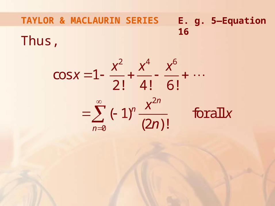
Thus,
2 4 6
2
0
cos 12! 4! 6!
( 1) for all(2 )!
nn
n
x x xx
xx
n
E. g. 5—Equation 16
TAYLOR & MACLAURIN SERIES
The Maclaurin series for ex, sin x, and cos x
that we found in Examples 2, 4, and 5 were
discovered by Newton.
These equations are remarkable because they say we know everything about each of these functions if we know all its derivatives at the single number 0.
TAYLOR & MACLAURIN SERIES
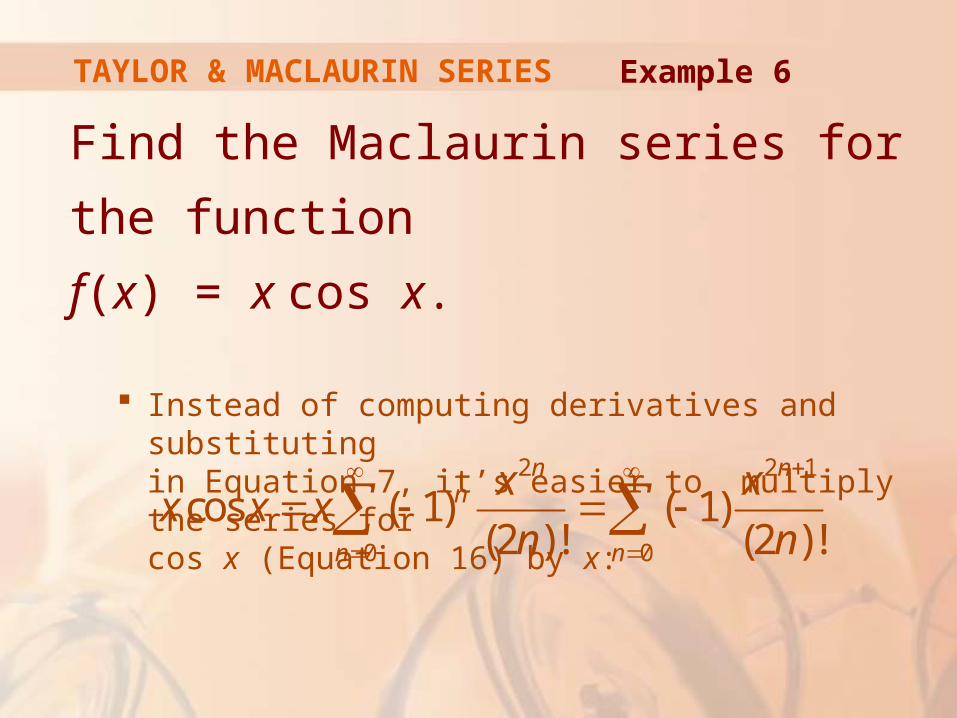
Find the Maclaurin series for the function
f(x) = x cos x.
Instead of computing derivatives and substituting in Equation 7, it’s easier to multiply the series for cos x (Equation 16) by x:
Example 6
2 2 1
0 0
cos ( 1) ( 1)(2 )! (2 )!
n nn
n n
x xx x x
n n
TAYLOR & MACLAURIN SERIES
Represent f(x) = sin x as
the sum of its Taylor series
centered at π/3.
Example 7
TAYLOR & MACLAURIN SERIES
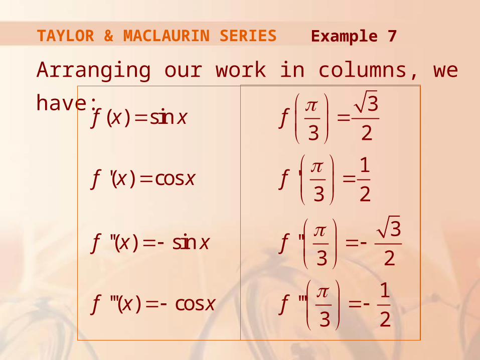
Arranging our work in columns, we have:
3( ) sin
3 2
1'( ) cos '
3 2
3''( ) sin ''
3 2
1'''( ) cos '''
3 2
f x x f
f x x f
f x x f
f x x f
Example 7

TAYLOR & MACLAURIN SERIES
That pattern repeats
indefinitely.
Example 7
TAYLOR & MACLAURIN SERIES
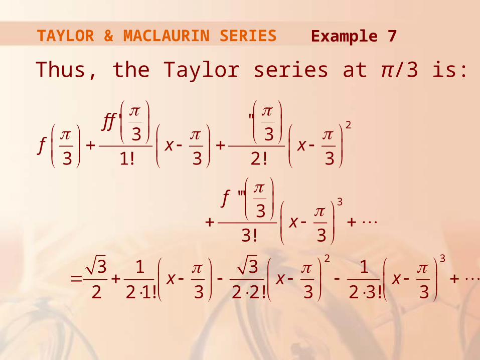
Thus, the Taylor series at π/3 is:
2
3
2 3
' ''3 3
3 1! 3 2! 3
'''3
3! 3
3 1 3 1
2 2 1! 3 2 2! 3 2 3! 3
f ff x x
fx
x x x
Example 7
TAYLOR & MACLAURIN SERIES
The proof that this series represents
sin x for all x is very similar to that in
Example 4.
Just replace x by x – π/3 in Equation 14.
Example 7
TAYLOR & MACLAURIN SERIES
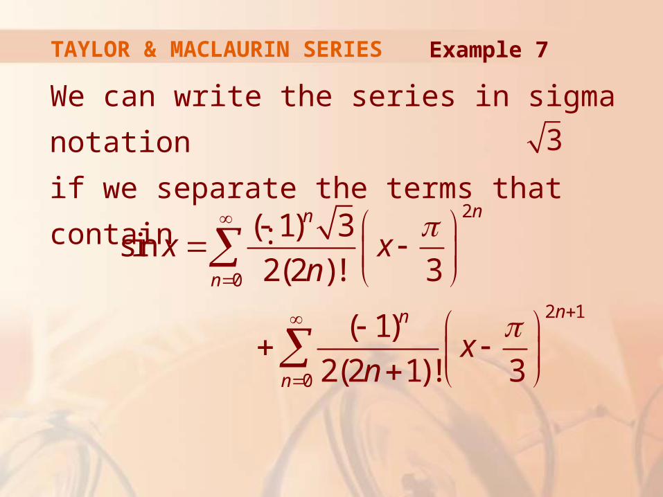
We can write the series in sigma notation
if we separate the terms that contain :
2
0
2 1
0
( 1) 3sin
2(2 )! 3
( 1)
2(2 1)! 3
nn
n
nn
n
x xn
xn
Example 7
3
TAYLOR & MACLAURIN SERIES
We have obtained two different series
representations for sin x, the Maclaurin
series in Example 4 and the Taylor series
in Example 7.
It is best to use the Maclaurin series for values of x near 0 and the Taylor series for x near π/3.
TAYLOR & MACLAURIN SERIES
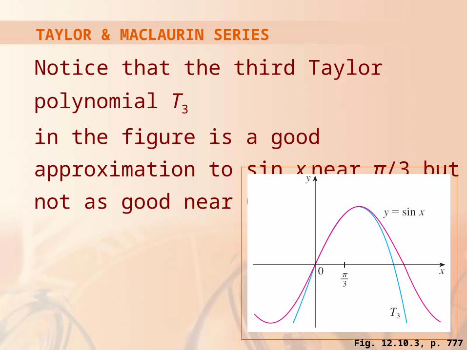
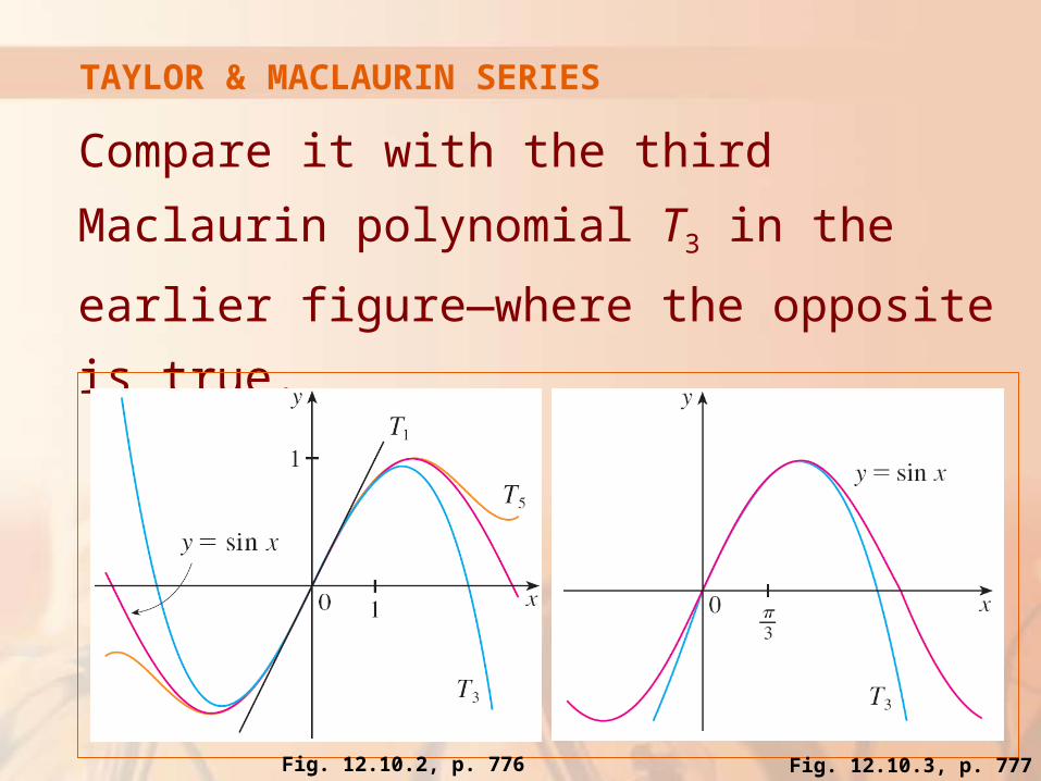
Notice that the third Taylor polynomial T3
in the figure is a good approximation to sin x
near π/3 but not as good near 0.
Fig. 12.10.3, p. 777
TAYLOR & MACLAURIN SERIES
Compare it with the third Maclaurin polynomial
T3 in the earlier figure—where the opposite is
true.
Fig. 12.10.3, p. 777Fig. 12.10.2, p. 776

TAYLOR & MACLAURIN SERIES
The power series that we obtained by indirect
methods in Examples 5 and 6 and in Section
11.9 are indeed the Taylor or Maclaurin series
of the given functions.
TAYLOR & MACLAURIN SERIES
That is because Theorem 5 asserts that,
no matter how a power series representation
f(x) = ∑ cn(x – a)n is obtained, it is always true
that cn = f (n)(a)/n!
In other words, the coefficients are uniquely determined.
TAYLOR & MACLAURIN SERIES
Find the Maclaurin series
for f(x) = (1 + x)k, where k
is any real number.
Example 8
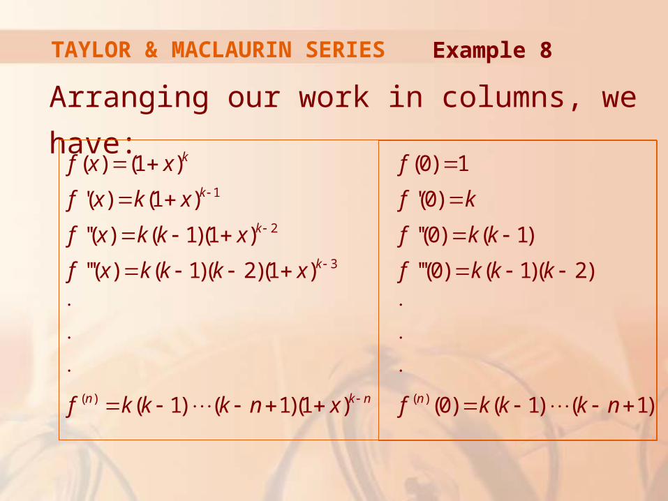
TAYLOR & MACLAURIN SERIES
Arranging our work in columns, we have:
1
2
3
( ) ( )
( ) (1 ) (0) 1
'( ) (1 ) '(0)
''( ) ( 1)(1 ) ''(0) ( 1)
'''( ) ( 1)( 2)(1 ) '''(0) ( 1)( 2)
( 1) ( 1)(1 ) (0) ( 1) ( 1)
k
k
k
k
n k n n
f x x f
f x k x f k
f x k k x f k k
f x k k k x f k k k
f k k k n x f k k k n
Example 8
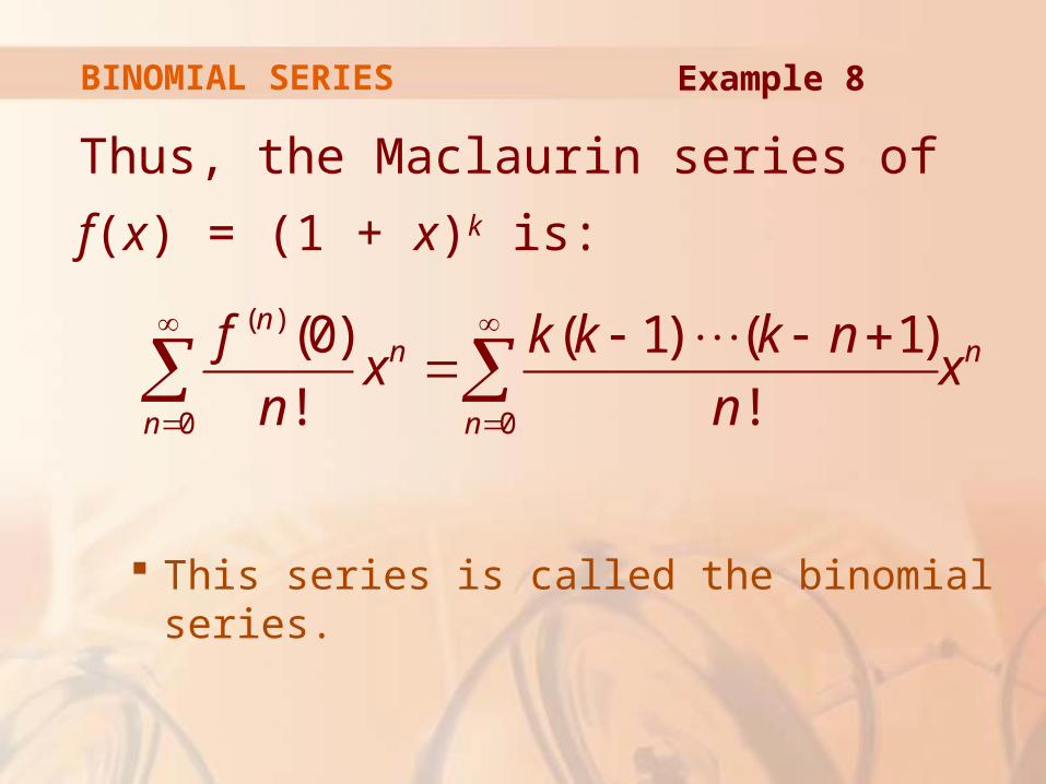
BINOMIAL SERIES
Thus, the Maclaurin series of f(x) = (1 + x)k
is:
This series is called the binomial series.
( )
0 0
(0) ( 1) ( 1)
! !
nn n
n n
f k k k nx x
n n
Example 8
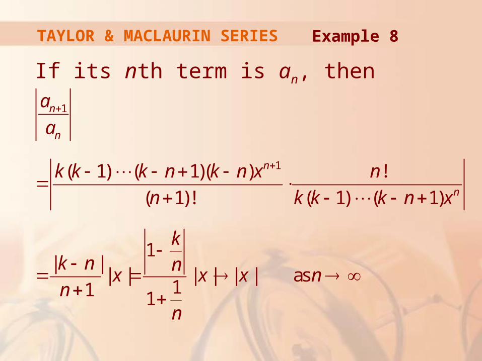
TAYLOR & MACLAURIN SERIES
If its nth term is an, then
1
1( 1) ( 1)( ) !
( 1)! ( 1) ( 1)
1| |
| | | | | | as11 1
n
n
n
n
a
a
k k k n k n x n
n k k k n x
kk n n
x x x nn
n
Example 8
TAYLOR & MACLAURIN SERIES
Therefore, by the Ratio Test,
the binomial series converges if |x| < 1
and diverges if |x| > 1.
Example 8
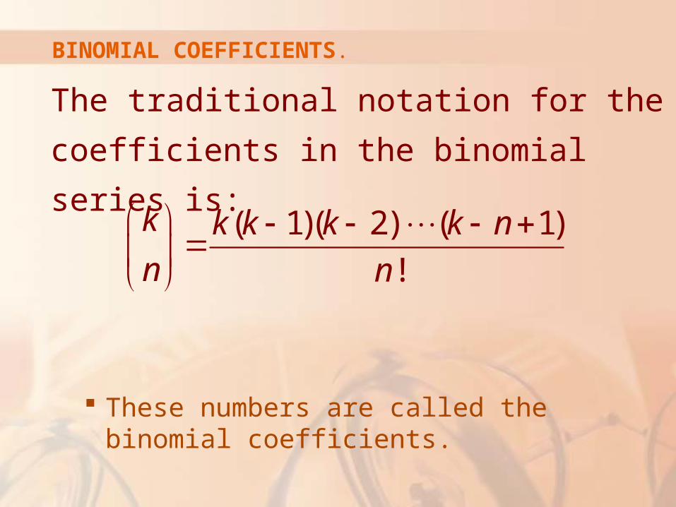
BINOMIAL COEFFICIENTS.
The traditional notation for the coefficients
in the binomial series is:
These numbers are called the binomial coefficients.
( 1)( 2) ( 1)
!
k k k k k n
n n
TAYLOR & MACLAURIN SERIES
The following theorem states that (1 + x)k
is equal to the sum of its Maclaurin series.
It is possible to prove this by showing that the remainder term Rn(x) approaches 0.
That, however, turns out to be quite difficult.
The proof outlined in Exercise 71 is much easier.
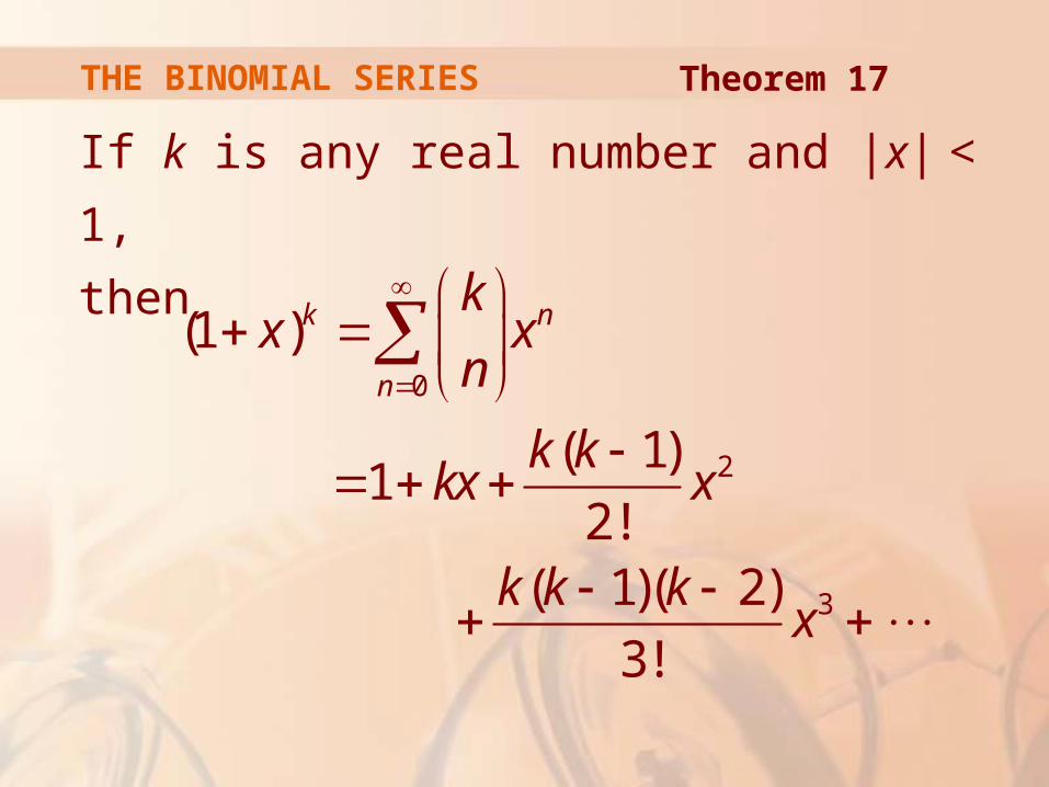
THE BINOMIAL SERIES
If k is any real number and |x| < 1,
then
Theorem 17
0
2
3
(1 )
( 1)1
2!( 1)( 2)
3!
k n
n
kx x
n
k kkx x
k k kx
TAYLOR & MACLAURIN SERIES
Though the binomial series always converges
when |x| < 1, the question of whether or not
it converges at the endpoints, ±1, depends on
the value of k.
It turns out that the series converges at 1 if -1 < k ≤ 0 and at both endpoints if k ≥ 0.
TAYLOR & MACLAURIN SERIES
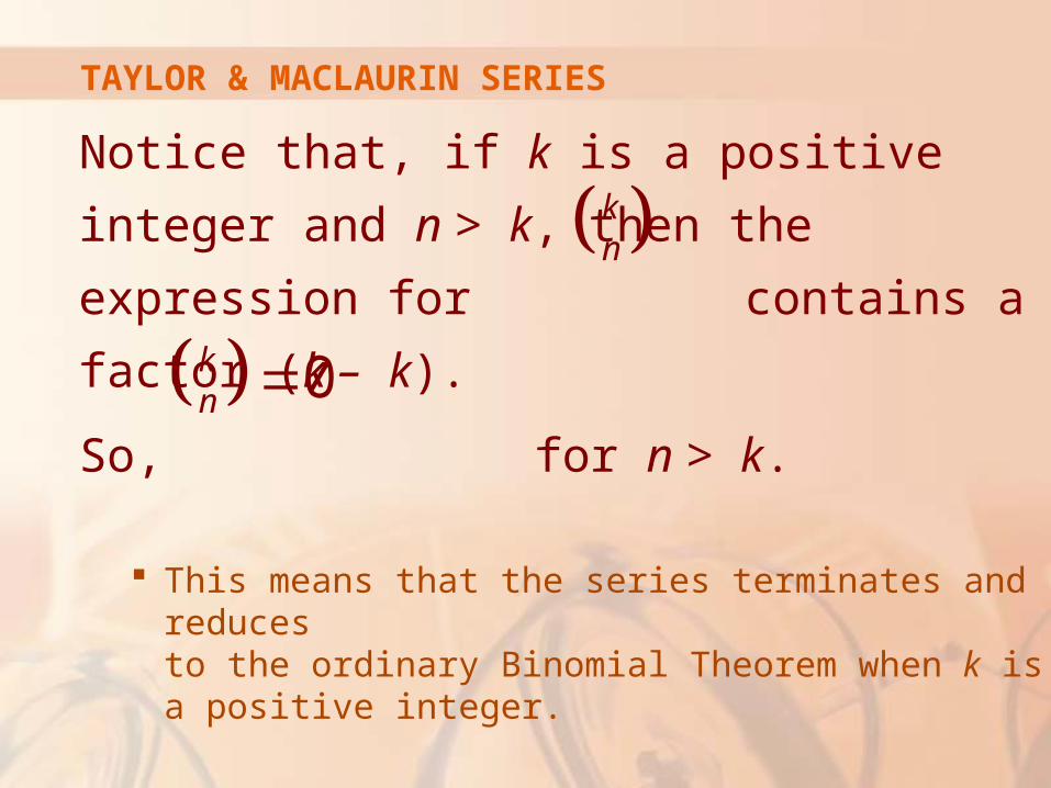
Notice that, if k is a positive integer and n > k,
then the expression for contains a factor
(k – k).
So, for n > k.
This means that the series terminates and reduces to the ordinary Binomial Theorem when k is a positive integer.
0kn
kn
TAYLOR & MACLAURIN SERIES
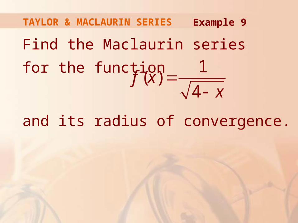
Find the Maclaurin series
for the function
and its radius of convergence.
Example 9
1( )
4f x
x
TAYLOR & MACLAURIN SERIES
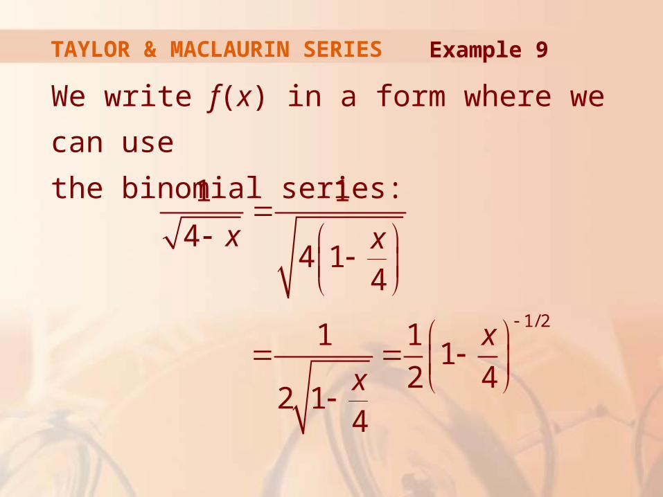
We write f(x) in a form where we can use
the binomial series:
1/ 2
1 1
44 1
4
1 11
2 42 1
4
x x
x
x
Example 9
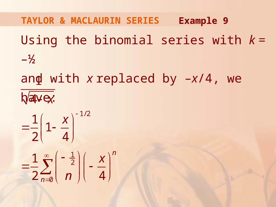
TAYLOR & MACLAURIN SERIES
Using the binomial series with k = –½
and with x replaced by –x/4, we have:
1/ 2
12
0
1
4
11
2 4
1
2 4
n
n
x
x
x
n
Example 9
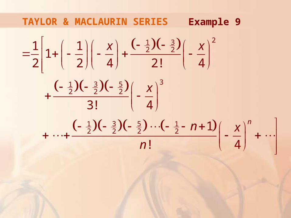
TAYLOR & MACLAURIN SERIES
2312 2
33 512 2 2
3 51 12 2 2 2
1 11
2 2 4 2! 4
3! 4
1
! 4
n
x x
x
n x
n
Example 9
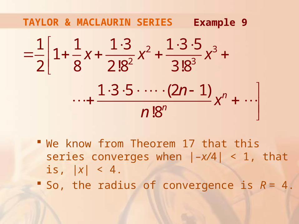
TAYLOR & MACLAURIN SERIES
We know from Theorem 17 that this series converges when |–x/4| < 1, that is, |x| < 4.
So, the radius of convergence is R = 4.
2 32 3
1 1 1 3 1 3 51
2 8 2!8 3!8
1 3 5 (2 1)
!8n
n
x x x
nx
n
Example 9
TAYLOR & MACLAURIN SERIES
For future reference, we collect some
important Maclaurin series that we have
derived in this section and Section 11.9,
in the following table.
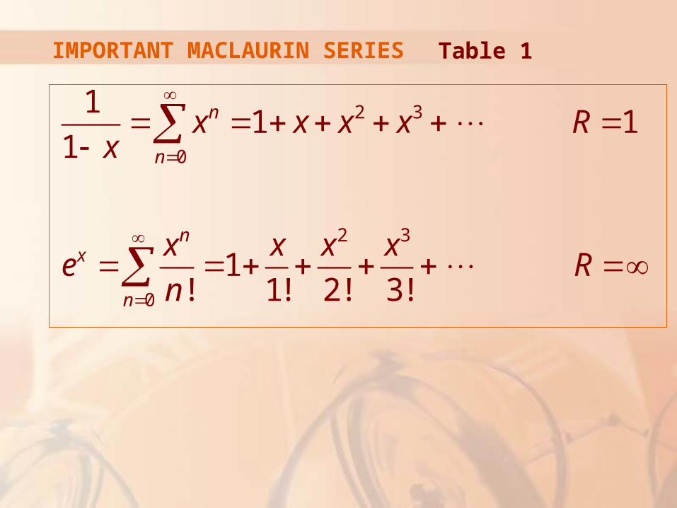
IMPORTANT MACLAURIN SERIES
2 3
0
2 3
0
11 1
1
1! 1! 2! 3!
n
n
nx
n
x x x x Rx
x x x xe R
n
Table 1
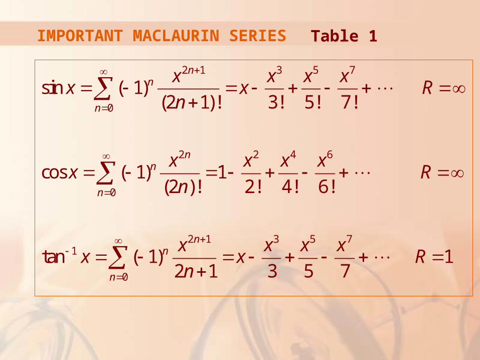
IMPORTANT MACLAURIN SERIES
2 1 3 5 7
0
2 2 4 6
0
2 1 3 5 71
0
sin ( 1)(2 1)! 3! 5! 7!
cos ( 1) 1(2 )! 2! 4! 6!
tan ( 1) 12 1 3 5 7
nn
n
nn
n
nn
n
x x x xx x R
n
x x x xx R
n
x x x xx x R
n
Table 1
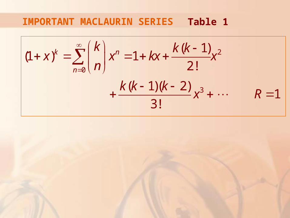
IMPORTANT MACLAURIN SERIES
2
0
3
( 1)(1 ) 1
2!
( 1)( 2)1
3!
k n
n
k k kx x kx x
n
k k kx R
Table 1
USES OF TAYLOR SERIES
One reason Taylor series are important
is that they enable us to integrate
functions that we couldn’t previously
handle.
USES OF TAYLOR SERIES
In fact, in the introduction to this chapter,
we mentioned that Newton often integrated
functions by first expressing them as power
series and then integrating the series term
by term.
USES OF TAYLOR SERIES
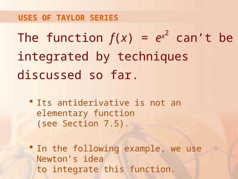
The function f(x) = ex2 can’t be integrated
by techniques discussed so far.
Its antiderivative is not an elementary function (see Section 7.5).
In the following example, we use Newton’s idea to integrate this function.
USES OF TAYLOR SERIES
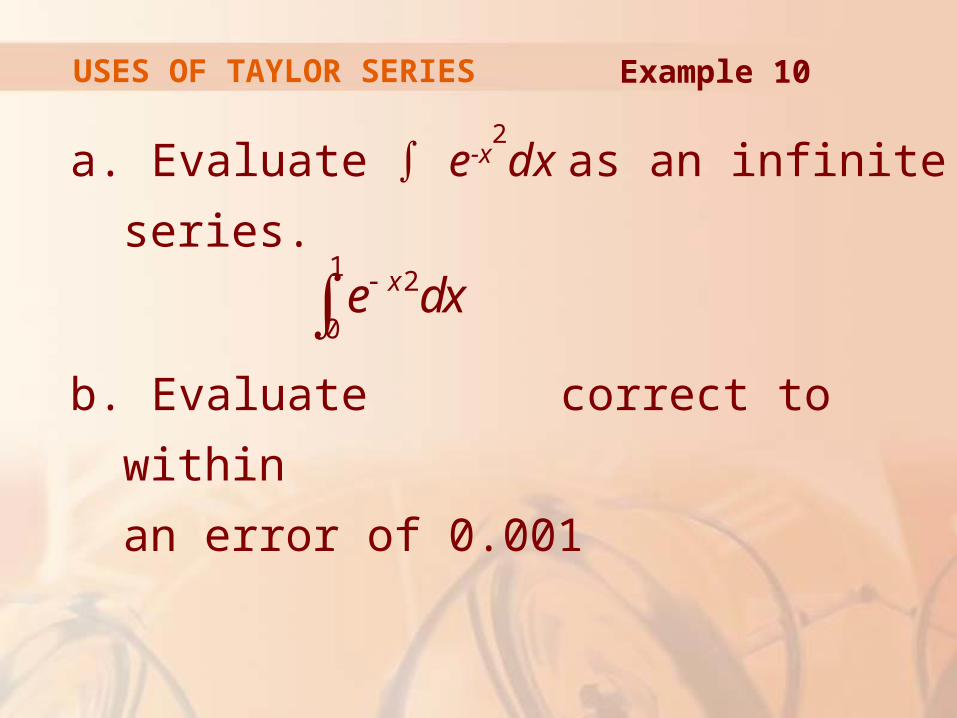
a. Evaluate ∫ e-x2dx as an infinite series.
b. Evaluate correct to within
an error of 0.001
Example 10
1 2
0
xe dx
USES OF TAYLOR SERIES
First, we find the Maclaurin series
for f(x) = e-x2
It is possible to use the direct method.
However, let’s find it simply by replacing x with –x2
in the series for ex given in Table 1.
Example 10 a
USES OF TAYLOR SERIES
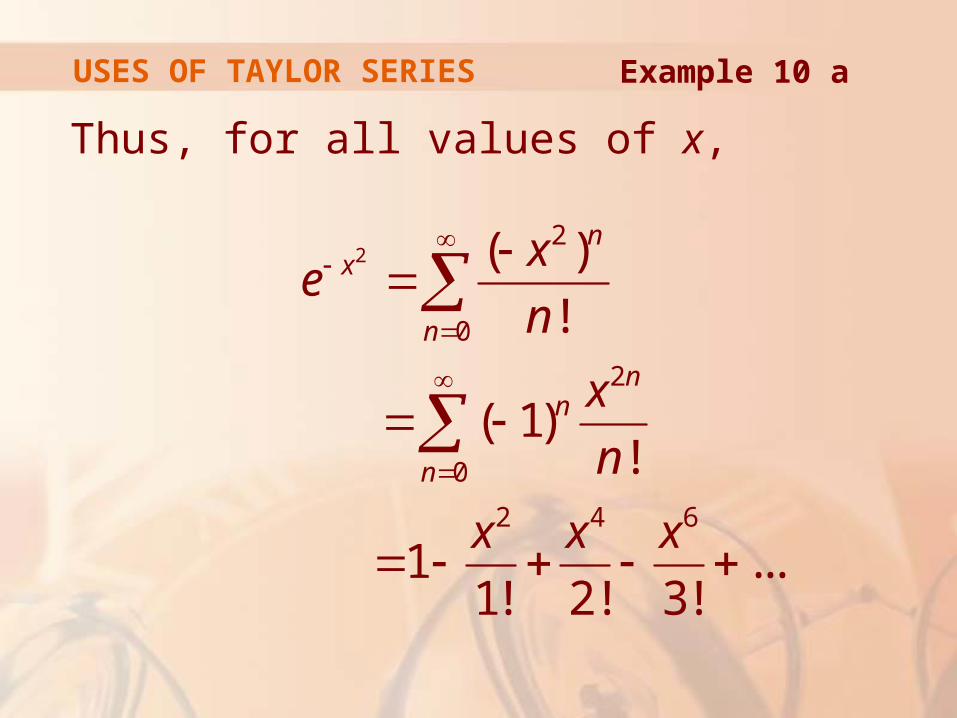
Thus, for all values of x,
Example 10 a
22
0
2
0
2 4 6
( )
!
( 1)!
1 ...1! 2! 3!
nx
n
nn
n
xe
n
x
n
x x x
USES OF TAYLOR SERIES
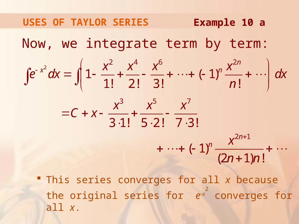
Now, we integrate term by term:
This series converges for all x because
the original series for e-x2 converges for all x.
22 4 6 2
3 5 7
2 1
1 ( 1)1! 2! 3! !
3 1! 5 2! 7 3!
( 1)(2 1) !
nx n
nn
x x x xe dx dx
n
x x xC x
x
n n
Example 10 a
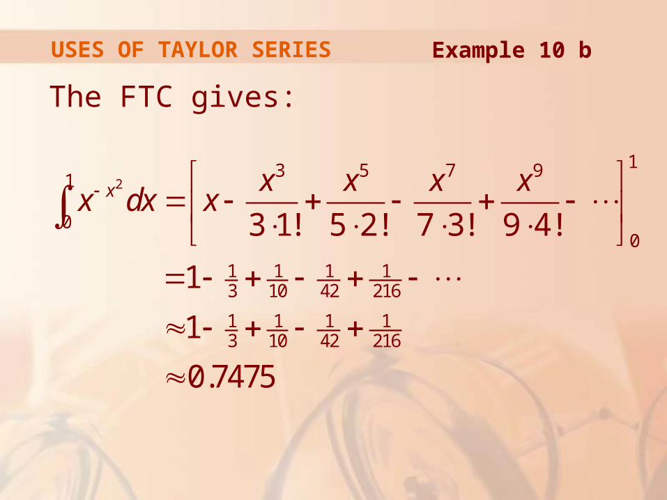
USES OF TAYLOR SERIES
The FTC gives:
Example 10 b
2
13 5 7 91
00
1 1 1 13 10 42 216
1 1 1 13 10 42 216
3 1! 5 2! 7 3! 9 4!
1
1
0.7475
x x x x xx dx x
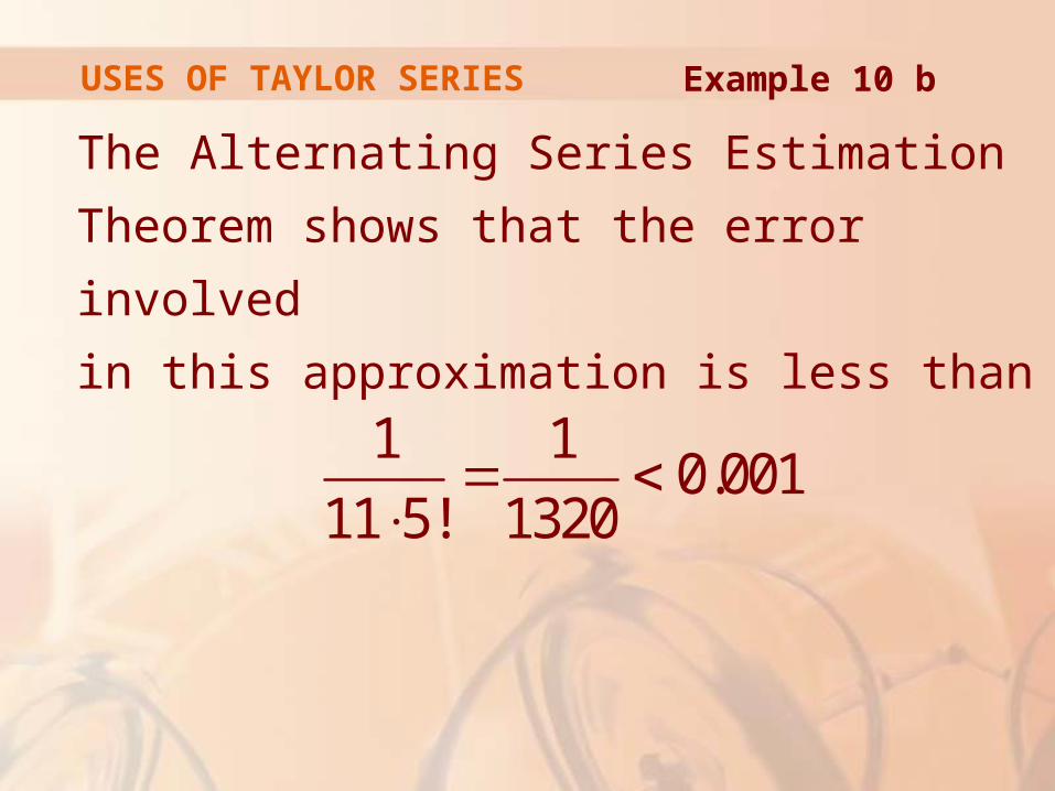
USES OF TAYLOR SERIES
The Alternating Series Estimation
Theorem shows that the error involved
in this approximation is less than
1 10.001
11 5! 1320
Example 10 b

USES OF TAYLOR SERIES
Another use of Taylor series is illustrated
in the next example.
The limit could be found with l’Hospital’s Rule.
Instead, we use a series.
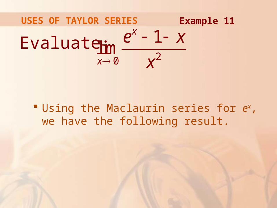
USES OF TAYLOR SERIES
Evaluate
Using the Maclaurin series for ex, we have the following result.
Example 11
20
1lim
x
x
e x
x
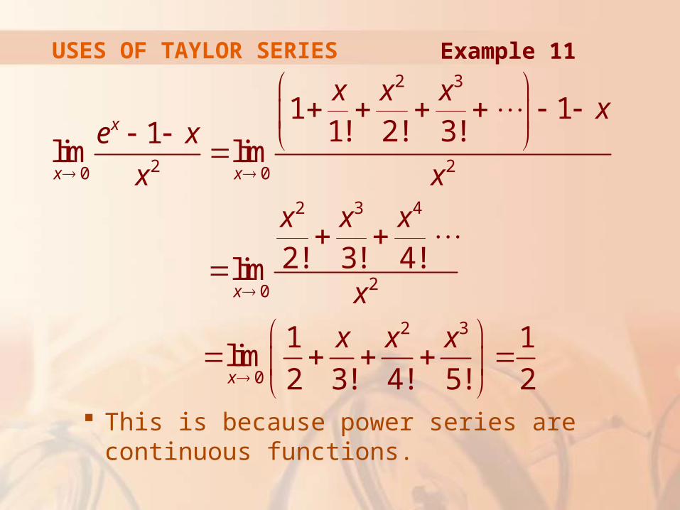
USES OF TAYLOR SERIES
This is because power series are continuous functions.
2 3
2 20 0
2 3 4
20
2 3
0
1 11! 2! 3!1
lim lim
2! 3! 4!lim
1 1lim
2 3! 4! 5! 2
x
x x
x
x
x x xx
e x
x x
x x x
x
x x x
Example 11
MULTIPLICATION AND DIVISION OF POWER SERIES
If power series are added or subtracted,
they behave like polynomials.
Theorem 8 in Section 11.2 shows this.
In fact, as the following example shows, they can also be multiplied and divided like polynomials.
MULTIPLICATION AND DIVISION OF POWER SERIES
In the example, we find only the first
few terms.
The calculations for the later terms become tedious.
The initial terms are the most important ones.
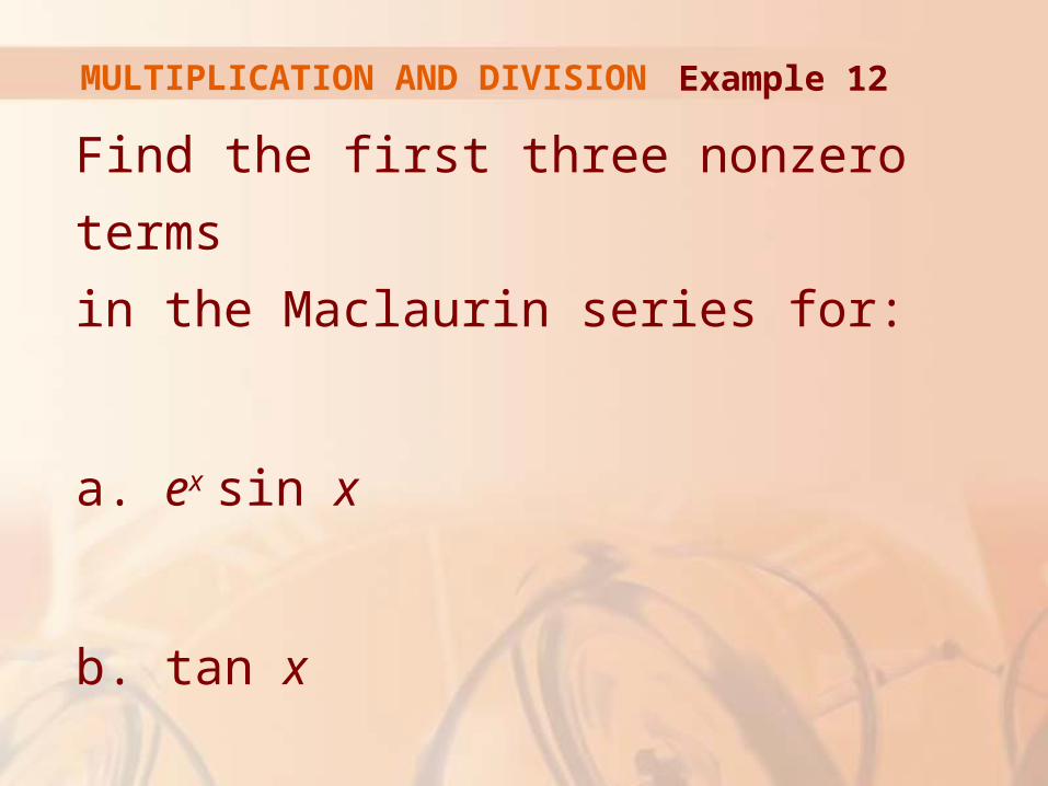
MULTIPLICATION AND DIVISION
Find the first three nonzero terms
in the Maclaurin series for:
a. ex sin x
b. tan x
Example 12
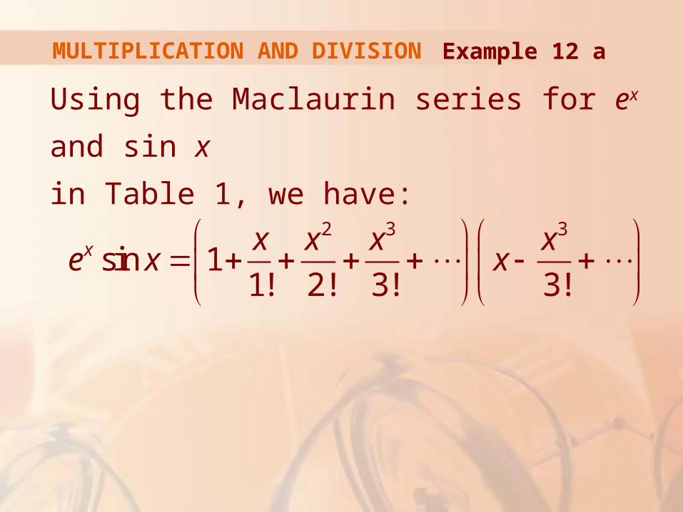
MULTIPLICATION AND DIVISION
Using the Maclaurin series for ex and sin x
in Table 1, we have:
Example 12 a
2 3 3
sin 11! 2! 3! 3!
x x x x xe x x
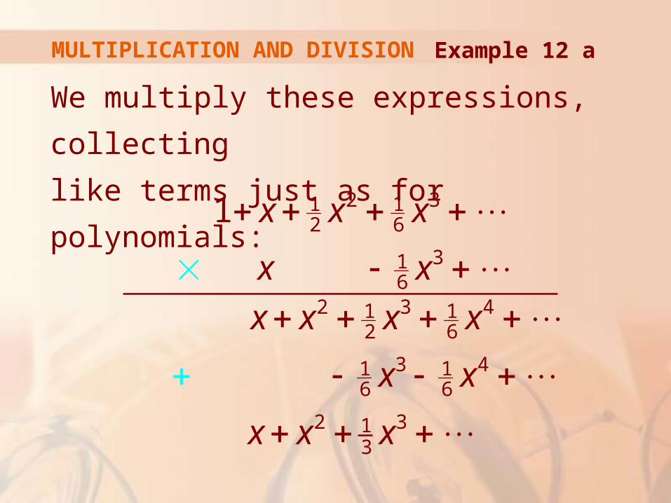
MULTIPLICATION AND DIVISION
We multiply these expressions, collecting
like terms just as for polynomials:
Example 12 a
2 31 12 6
316
2 3 41 12 6
3 41 16 6
2 313
1 x x x
x x
x x x x
x x
x x x
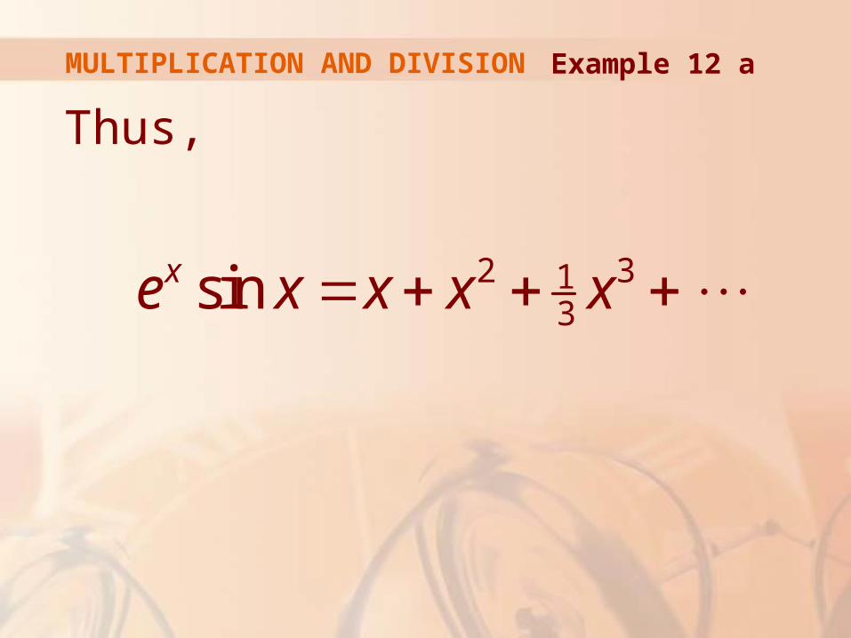
MULTIPLICATION AND DIVISION
Thus,
Example 12 a
2 313sinxe x x x x
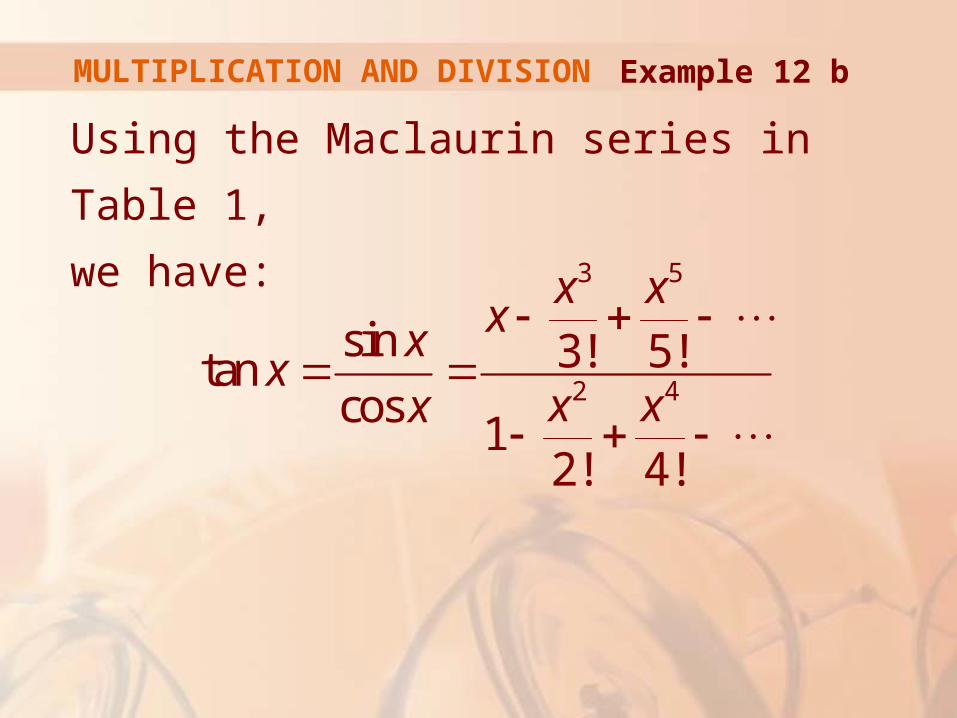
MULTIPLICATION AND DIVISION
Using the Maclaurin series in Table 1,
we have:
Example 12 b
3 5
2 4
sin 3! 5!tancos
12! 4!
x xxx
xx xx
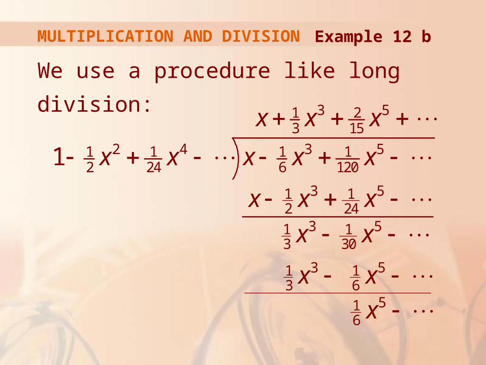
MULTIPLICATION AND DIVISION
We use a procedure like long division:
Example 12 b
3 51 23 15
2 4 3 51 1 1 12 24 6 120
3 51 12 24
3 51 13 30
3 51 13 6
516
1
x x x
x x x x x
x x x
x x
x x
x
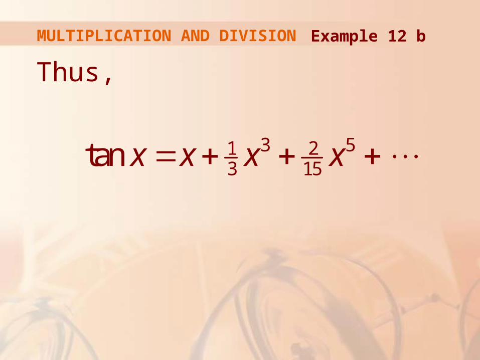
MULTIPLICATION AND DIVISION
Thus,
Example 12 b
3 51 23 15tan x x x x
MULTIPLICATION AND DIVISION
Although we have not attempted to
justify the formal manipulations used in
Example 12, they are legitimate.
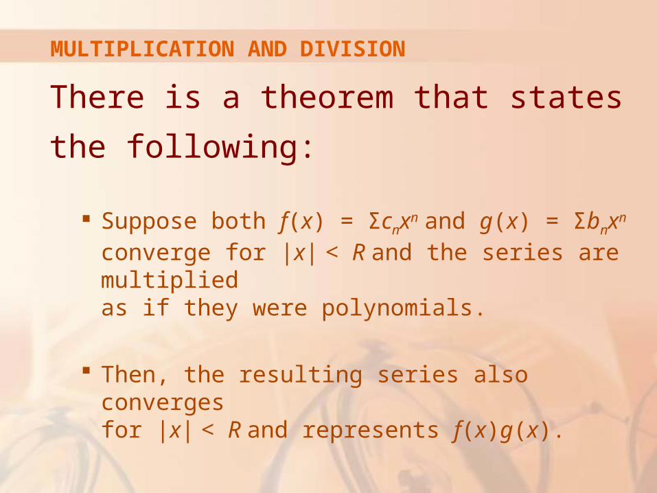
There is a theorem that states
the following:
Suppose both f(x) = Σcnxn and g(x) = Σbnxn converge for |x| < R and the series are multiplied as if they were polynomials.
Then, the resulting series also converges for |x| < R and represents f(x)g(x).
MULTIPLICATION AND DIVISION
For division, we require b0 ≠ 0.
The resulting series converges for sufficiently small x.
MULTIPLICATION AND DIVISION