12 - IntechOpen

12

Performance Evaluation of Potential Field based Distributed Motion Planning Methods for Robot

Collectives

Leng-Feng Lee and Venkat N. Krovi University at Buffalo

USA

1. Introduction

In the past decade, ongoing revolutions in computing effectiveness and miniaturization of processors/sensors/actuators have facilitated the transition of research focus from an individual mobile robot to networked distributed teams of mobile robots. The development of effective motion-planning methods for such collectives is critical to realizing the full potential of the group in numerous applications ranging from reconnaissance, foraging, herding to cooperative payload transport. While considerable literature exists for motion planning of individual mobile agents, the renewed challenge lies in creating motion plans for the entire team while incorporating notions such as cooperation. The “formation” paradigm has emerged as a convenient mechanism for abstraction and coordination with approaches ranging from leader-following (Wang, 1991; Desai et al., 2001), virtual structures (Lewis and Tan, 1997; Beard et al., 2001) and virtual leaders (Leonard and Fiorelli, 2001; Ogren et al., 2002). The group control problem now reduces to a well-known single-agent control problem from which the other agents derive their control laws but requires communication of some coordination information. Early implementations involved the kinematic specification of the followers’ motion-plans as a “prescribed motions” relative to a team-leader without the ability to affect the dynamics of the leader. Subsequent approaches have incorporated some form of “formation-feedback” from the members to the overall group using natural or artificially introduced dynamics within the constraints. The formation paradigm has evolved to allow prescription of parameterized formation maneuvers and group feedback (Egerstedt and Hu, 2001; Young et al., 2001; Ogren et al., 2002). From these seemingly disparate approaches, a dynamic system-theoretic perspective has emerged for examining the decentralized multi-agent “behavioral control” in the context of “formations” (Lawton et al., 2000; Egerstedt and Hu, 2001; Leonard and Fiorelli, 2001; Young et al., 2001; Ogren et al., 2002; Olfati-Saber and Murray, 2006). “Behavioral” control laws, derived implicitly as gradients of limited-range artificial potentials, can be implemented in a decentralized manner while permitting a Lyapunov-based analysis of formation maintenance. Various variants of the Artificial Potential Field (APF) framework have been leveraged in implementing such behavioral motion-planning/control of robot collectives due to their seeming ease of formulation, decentralization and scalability. However, we note that while

www.intechopen.com

Mobile Robots Motion Planning, New Challenges

228

stability guarantees (typically asymptotic) may be obtained, APF approaches are unable to guarantee strict formation maintenance. Such strict formation maintenance is critical in applications such as cooperative payload transport by collectives (Bhatt et al., 2008) or in distributed sensor deployment applications where the robots are to form some geometric pattern and maintain it while moving about in the world (Young et al., 2001). We note that the group of independent mobile robots moving together in formation and coupled together by constraint dynamics can alternatively be viewed as a constrained mechanical system. The computation of motion plans for such collectives in a potential field may also be viewed as simulating the forward dynamics of a constrained multi-body mechanical system. By doing so, we would like to link (and leverage) the extensive literature on formulation and implementation of computational simulation of multibody systems (Haug, 1989; Shabana, 1989; Schiehlen, 1990; García de Jalón and Bayo, 1994; Ascher and Petzold, 1998) to the problem of motion planning of mobile robot collectives. In this chapter, we evaluate the formation maintenance performance of several formulations developed by analogy to the approaches used for constrained mechanical systems. These include: (i) a direct Lagrangian multiplier elimination approach (to serve as the benchmark); (ii) a penalty-formulation approach which is the most popular implementation; and (iii) a constraint manifold projection approach. We note that the instabilities introduced in the form of the “formulation stiffness” at the algorithm development stage have the potential to hinder the subsequent control and requires a careful quantitative examination (Ascher et al., 1997). Hence, we compare and contrast the various approaches on the basis of modular formulation, distributed computation and relative computational efficiency and accuracy. These aspects are studied in the context of the motion-planning of a group of point-mass mobile robots which are constrained together by means of rheonomous holonomic constraints. The rest of the paper is organized as follows: Section 2 presents a brief discussion of various candidate formulations of forward dynamics approaches for constrained multibody systems. In Section 3, the dynamic model of the system of point-mass robots moving in plane is introduced and the candidate methods are evaluated from viewpoint of distribution of computation. Section 4 discusses the standardized test arena and the performance evaluation metric which is then used in Section 5 to compare and contrast the methods. Section 6 presents a brief discussion and concluding remarks.

2. Forward Dynamics Formulations for Constrained Mechanical Systems

In this section we briefly review some of the available alternative formulations for developing the forward dynamics simulations in constrained mechanical systems. At the outset, we note that suitable selection of a set of configuration coordinates is of particular importance due to its impact both on the ease of formulation and the subsequent computational efficiency. We make use of expanded sets of dependent Cartesian coordinates linked together by holonomic constraints as being most appropriate for modular composition and general-purpose analysis. The overall dynamics can be formulated as a system of ODEs whose solutions are required to satisfy additional holonomic (algebraic) constraint equations as Lagrangian equations of the first kind (Arnold, 1989):

www.intechopen.com

Performance Evaluation of Potential Field based Distributed Motion Planning Methods for Robot Collectives

229

υ=$##

q (1)

( ) ( ) ( )υ υ λ= −$# # # ## # # #

, , , TM q f q u t A q (2)

( )=# ##, 0C q t (3)

where q#

is the n -dimensional vector of generalized coordinates.

υ#

is the n -dimensional vector of generalized velocities.

( )M q#

is the n n× dimensional inertia matrix.

( ), , ,f q u tυ# ## #

is the n -dimensional vector of external forces.

#u is the vector of actuator forces/torques.

( ),C q t# #

is the m -dimensional vector of holonomic constraints.

( )A q C q=∂ ∂## #

is the m n× dimensional constraint Jacobian matrix.

λ#

is the m -dimensional vector of Lagrange multipliers.

The solution of resulting system of index-3 Differential Algebraic Equations (DAEs) by direct finite difference discretization is not possible using explicit discretization methods. We adopt a converted ODE approach, wherein all the algebraic position and velocity level constraints are differentiated and represented at the acceleration level to obtain an augmented index-1 DAE (in terms of both, the unknown accelerations and the unknown multipliers). Differentiating the position constraints in Eq.(3), with respect to time, yields the velocity-level constraints:

= =$# # #

0C Av (4)

Further differentiation with respect to time yields the acceleration level constraints as:

= + =$$ $$# # # #

0C Av Av (5)

Thus, Eq. (2) can then be written together with Eq. (5) as an index-1 DAE as:

( ) ( ) ( ) ( )λ

+ ×+ × + + ×

⎡ ⎤⎡ ⎤ ⎡ ⎤ ⎢ ⎥⎢ ⎥ ⎢ ⎥ = ⎢ ⎥⎢ ⎥ ⎢ ⎥ −⎢ ⎥ ⎢ ⎥⎣ ⎦⎣ ⎦ ⎣ ⎦

$# #$# #1 1

0

T

n mn m n m n m

fvM A

A Av (6)

In a typical forward dynamics simulation setting, the index-1 DAE systems resulting from the converted ODE approach are then converted into final system of first-order ODEs by: (a)

www.intechopen.com


230

direct Lagrange multiplier elimination; (b) penalty-formulation; or (c) constraint manifold projection.

2.1 Direct Lagrange Multiplier Elimination

In this approach, a simultaneous solution of the augmented linear system of Eq. (6) is obtained at each time step. While an explicit inversion of the augmented system may be avoided by adopting a Gaussian elimination method, the overall approach may still be denoted as:

( )( )λ

− ⎡ ⎤⎡ ⎤⎡ ⎤⎡ ⎤ ⎢ ⎥⎢ ⎥⎢ ⎥⎢ ⎥ ⎢ ⎥= =⎢ ⎥⎢ ⎥⎢ ⎥ ⎢ ⎥−⎢ ⎥ ⎢ ⎥⎣ ⎦ ⎣ ⎦ ⎣ ⎦ ⎢ ⎥⎣ ⎦

$ ## ## #$# # ## #

11

2

,

0 ,

T f q vfv M A

A Av f q v (7)

Thus, the overall system may now be written as a system of first order ODEs as:

( )υ

υ×

××

⎡ ⎤⎡ ⎤ ⎢ ⎥⎢ ⎥= = ⎢ ⎥⎢ ⎥ ⎢ ⎥⎢ ⎥⎣ ⎦ ⎣ ⎦

$#$ #$$### # #

1

2 11 1 ,

n

nn

qx

q f q (8)

which may then be integrated using standard numerical solvers. The main advantage is its conceptual simplicity and simultaneous determination of the accelerations and the Lagrange multipliers by solving a linear system of equations. However, this is a centralized approach and does not scale up very well.

2.2 Penalty-Formulation

In penalty-based approaches the holonomic constraints are relaxed and replaced by linear/non-linear virtual springs and dampers, thereby incorporating the constraint equations as a dynamical system penalized by a large factor. The Lagrange multipliers are approximated using a virtual spring type law (based on the extent of the constraint violation and assumed spring stiffness) and eliminated from the list of +n m unknowns leaving

behind a system of 2n first order ODEs. While the sole initial drawback may appear to be

restricted to the numerical ill-conditioning due to selection of large penalty factors, it is important to note that penalty approaches only approximate the true constraint forces and can create unanticipated problems (as will be discussed later). This individual multiplier

values can be explicitly calculated as λ = + $i ii P i D iK C K C where

iPK is the spring constant,

iDK is the damping constant and ( )#

iC q is the constraint violation in the direction of the

respective λi . By substituting the value of λ#

in Eq. (2), the final ODE system can be written

as:

( )( )×

× −×

⎡ ⎤⎡ ⎤ ⎢ ⎥⎢ ⎥= = ⎢ ⎥⎢ ⎥ − +⎢ ⎥⎢ ⎥⎣ ⎦ ⎣ ⎦

$#$ # $$$## ## #

1

2 1 11

n

n Tn P D

vqx

q M f A K C K C (9)

www.intechopen.com


231

where ⎡ ⎤= ⎢ ⎥⎣ ⎦iP PK diag K and ⎡ ⎤= ⎢ ⎥⎣ ⎦iD DK diag K .

2.3 Constraint Manifold Projection

This approach seeks to take the dynamical equations with constraint-reactions into the

tangent and cotangent subspace. The rheonomous holonomic constraints, ( )=# ##, 0C q t , can be

written in differential form as:

( )⎡ ⎤ ⎡ ⎤∂ ∂⎢ ⎥ + = ⇔ =⎢ ⎥⎢ ⎥ ⎢ ⎥∂ ∂⎣ ⎦⎢ ⎥⎣ ⎦

$ $# # # ## # ##

0C C

q Aq a qq t

(10)

Let ( )#

S q be an ( )× −n n m dimensional full rank matrix whose column space is in the null

space of A i.e. 0AS=#

. The orthogonal subspace is spanned by the so-called constraint

vectors (forming the rows of the matrix A ) while the tangent subspace complements this orthogonal subspace in the overall generalized velocity vector space. All feasible dependent

velocities, q$#

, of a constrained multibody system necessarily belong to this tangent space,

appropriately called the space of feasible motions. This space is spanned by the columns of S )

and is parameterized by an ( )n m− -dimensional vector of independent velocities, ( )tν#

,

yielding the expression for the feasible dependent velocities as:

( ) ( )ν η= = +$## ## #

q v S t q (11)

where ( )η# #

q is the particular solution of (10). Differentiating this further we get:

( )ν ν η ν γ ν= + + = +$$ $ $ $# # # ## ## #

,v S S S q (12)

where ( )γ ν ν η= +$ $# ## ##

,q S needs to be calculated numerically which has potential of

introducing errors. In order to avoid this situation, we adopted the method in (Yun and Sarkar, 1998). Such a projection process works out well in a Riemannian setting (where the notion of orthogonal complement subspaces exists). Special care needs to be exercised when treating

configuration spaces such as ( )2SE or ( )3SE . A family of projections exists depending on

selection of dependent/independent velocities. However, once a projection is selected, the dynamic equations of motion can now be projected on to the instantaneous feasible motion directions, to obtain the so-called constraint-reaction-free equations of motion. Pre-

multiplying both sides of Eq. (2) by TS and noting that =#0T TS A we get:

www.intechopen.com


232

=$# #

T TS Mv S f (13)

By substituting υ$ from Eq. (12) into Eq. (13) and solving for $v we get:

( ) ( )1T T TS MS S M S fν γ−

=− −$# # #

(14)

The resulting overall system of ODEs may be expressed in state-space form as:

( )( ) ( ) ( )

ν η

ν γ

×−− ×

− ×

⎡ ⎤+⎡ ⎤ ⎢ ⎥⎢ ⎥= = ⎢ ⎥⎢ ⎥ − −⎢ ⎥⎢ ⎥⎣ ⎦ ⎣ ⎦

$ # #$ #$## # #

112 1

1

n

n m T T Tn m

Sqx

S MS S M S f (15)

The final solution may be obtained either by numerically integrating a system of 2n m−

first-order ODEs in the n dependent velocities and −n m independent accelerations.

2.4 Baumgarte Stabilization

The drawbacks of the Constraint Manifold Projection approach include: (i) the need to provide additional consistent initial conditions; and (ii) the mild instability of the differentiated constraints resulting in state-drift from the position-level constraint manifold. While the growth rate can be reduced by lowering the error tolerance and by using smaller step-sizes or greater numerical precision, this comes at the cost of longer and more expensive computations. Baumgarte stabilization (Baumgarte, 1983) involves the creation of an artificial first or second-order dynamical system which has the algebraic position-level constraint as its attractive equilibrium configuration. For example, when the holonomic constraints in Eq. (3) are approximated by a first order system of the form, we obtain:

( ) ( )σ σ+ = >$# # ## #

, , 0, 0C q t C q t (16)

where σ is the rate of convergence. The equilibrium condition for this first order system is

the constraint manifold ( )=# ##, 0C q t and for any initial condition ( )0q

#, which may not satisfy

the holonomic constraint equation ( )( )0 0C q =# ##

, the above first order equation guarantees

exponential convergence of ( )( )=# ##0C q t to zero as the time t progresses. The rate of

convergence will be determined by σ , which can be chosen based on specific application. Eq. (16) can be suitably modified as:

( )σ⎡ ⎤ ⎡ ⎤∂ ∂⎢ ⎥ =− − ⇔ =⎢ ⎥⎢ ⎥ ⎢ ⎥∂ ∂⎣ ⎦⎢ ⎥⎣ ⎦

$ $# ## ## # ##

C Cq C Aq a q

q t (17)

and the rest of solution process remains unchanged. While Baumgarte’s technique is very popular in the engineering application community, principally due to the resulting

www.intechopen.com


233

augmented ODE formulation, the practical selection of the parameters of the stabilization system depends both on the discretization methods and step-size and is widely regarded as an open research problem (Ascher et al., 1995).

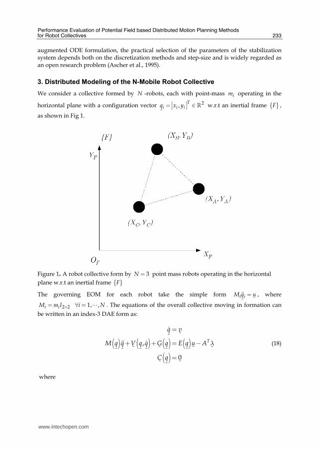
3. Distributed Modeling of the N-Mobile Robot Collective

We consider a collective formed by N -robots, each with point-mass im operating in the

horizontal plane with a configuration vector [ ]= ∈{#

2,T

i i iq x y w.r.t an inertial frame { }F ,

as shown in Fig 1.

Figure 1. A robot collective form by = 3N point mass robots operating in the horizontal

plane w.r.t an inertial frame { }F

The governing EOM for each robot take the simple form =$$##

i iM q u , where

×= ∀ = A2 2 1, ,i iM m I i N . The equations of the overall collective moving in formation can

be written in an index-3 DAE form as:

( ) ( ) ( ) ( )( )

λ

=

+ + = −

=

$##

$$ $# # # ## # # # # #

# ##

,

0

T

q v

M q q V q q G q E q u A

C q

(18)

where

www.intechopen.com


234

1

;

N

q

q

q

⎡ ⎤⎢ ⎥⎢ ⎥= ⎢ ⎥⎢ ⎥⎢ ⎥⎣ ⎦

#B

##

( )[ ]

[ ]

1 2 2

2 2

0

;

0 N

M

M q

M

×

×

⎡ ⎤⎢ ⎥⎢ ⎥= ⎢ ⎥⎢ ⎥⎢ ⎥⎣ ⎦

A#

B D B# A

#

( )Tq pu k V=− ∇##

; ( ) 2 2N NE q I ×=#

; ( ) 0G q =##

;

( ), 0V q q =$## #

We will consider the case where a rigid formation is desired. The 2 3N− constraint equations

(Olfati-Saber and Murray, 2002) that maintain the rigidity are obtained from the requirement that each robot tries to maintain a desired distance with the others:

( ) ( )(2 3) 1

0ijN

C q C q− ×

⎡ ⎤= =⎢ ⎥⎣ ⎦ ## # (19)

Equation (18) represents the centralized form of the governing equations using artificial potentials. We now consider the possibility of distributing the motion-planning computations between the multiple agents. Further details are available in Lee (2004).

3.1 The Penalty Formulation

Noting that the state vector TT T T

A B Cq q q q⎡ ⎤= ⎢ ⎥⎣ ⎦# # # # has state variables belonging to each of the

robots ,A B and C , the distributed model may be obtained in state-space form as:

[ ] ( )( )14 1; , ,

i i

ii

i Ti i i i i P i D i

qx i A B C

q M E u A K C K C

υ−×

⎡ ⎤⎡ ⎤ ⎢ ⎥⎢ ⎥= = ∀ =⎢ ⎥⎢ ⎥ − +⎢ ⎥⎢ ⎥⎣ ⎦ ⎣ ⎦

$#$ # $$$#

# # ##

(20)

where iPK ,

iDK are the compliance and damping matrices and iC#

represents the extent of

the constraint violation as pertinent to robot i .

The three dynamic sub-systems, shown in Eq. (20), can be simulated in a distributed manner

if at every time step: (i) either the information pertaining to ( )iC q# #

, the extent of the

constraint violation, is made available explicitly or (ii) computed by exchanging state information between the robots. The sole coupling between the two sub-parts is due to the Lagrange multipliers, which are now explicitly calculated using the virtual spring. While this is shown for a “three robot system”, the process generalizes easily for “N-robot” system.

3.2 Constraint Manifold Projection

We examine this approach as an appropriate alternative to the penalty formulation where again our emphasis is on distribution of the motion planning computations to be performed

by the individual robots. Noting that the state vector may be written as TT T T

A B Cq q q q⎡ ⎤= ⎢ ⎥⎣ ⎦# # # #,

the projected dynamics equations may be partitioned as:

www.intechopen.com


235

[ ]6 6

0 0

0 0

0 0

0 0

0 0

0 0

TAA

T T T TA B C B B

TC C

T TA AA

T T T T T T T TA B C B B A B C B

T TC C C

SM

S S S M S v

M S

uM

S S S M S S S I u

M u

γ

γ

γ

×

⎡ ⎤⎡ ⎤ ⎢ ⎥⎢ ⎥ ⎢ ⎥⎡ ⎤ ⎢ ⎥ ⎢ ⎥ +⎢ ⎥ ⎢ ⎥⎣ ⎦ ⎢ ⎥⎢ ⎥ ⎢ ⎥⎣ ⎦ ⎢ ⎥⎣ ⎦⎡ ⎤ ⎡ ⎤⎡ ⎤ ⎢ ⎥ ⎢ ⎥⎢ ⎥ ⎢ ⎥ ⎢ ⎥⎡ ⎤ ⎡ ⎤⎢ ⎥ ⎢ ⎥ ⎢ ⎥=⎢ ⎥ ⎢ ⎥⎢ ⎥⎣ ⎦ ⎣ ⎦⎢ ⎥ ⎢ ⎥⎢ ⎥ ⎢ ⎥ ⎢ ⎥⎣ ⎦ ⎢ ⎥ ⎢ ⎥⎣ ⎦ ⎣ ⎦

$#

######

(21)

Thus, it is now possible to calculate the state vectors forming separately as:

( ) ( )( )1 ; , ,

i iii T T

i i i i i i

Sqx i A B C

S MS S M E u

ν η

ν γ−

⎡ ⎤+⎡ ⎤ ⎢ ⎥⎢ ⎥= = ∀ =⎢ ⎥⎢ ⎥ ⎢ ⎥− −⎢ ⎥⎣ ⎦ ⎢ ⎥⎣ ⎦

$ #$ ## $# ##

(22)

By examining Eq. (21), we note that the overall system can be evaluated in a distributed

manner if states iq#

and iν# are made available. Each independent sub-part can now be

numerically integrated on a mobile robot thereby permitting independent operation. At each time-instant, the complete state of the system needs to be exchanged between the

robots. The coupling between the various sub-parts is due to the existence of the ( ) 1TS MS−

.

This matrix inverse needs to be computed on each and every processor (although we note that the explicit calculation of the inverse is typically avoided by using an optimal equation solver). Alternatively, state information from the slave processors could be collected by a

central processor at each time instant, the ( ) 1TS MS−

computed and the result subsequently

broadcasted to all robots.

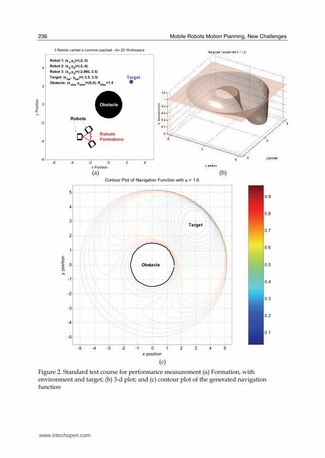
4. The Standardized Test Arena

In order to compare the performance of various methods for motion planning of robot collectives within a potential-field framework, we developed a standardized test course. A graphical user interface (GUI) is used to locate the positions of the initial robot configurations, the obstacles and the target. As shown in Figure 2(a). Then an APF is developed in the form of a navigation function (Rimon and Koditschek, 1992) to ensure a unique minimum. This is shown as a 3D plot in Figure 2(b) and as a contour plot in Figure 2(c).

www.intechopen.com


236

-6 -4 -2 0 2 4-6

-4

-2

0

2

4

Robots

Robot 1: (x1,y

1)=(-2,-3)

Robot 2: (x2,y

2)=(-2,-4)

Robot 3: (x3,y

3)=(-2.866,-3.5)

Target: (xtar

, ytar

)=( 2.5, 2.5)

Obstacle: (xobs

,yobs

)=(0,0); Robs

=1.5

Robots

Formations

Obstacle

Target

3 Robots carried a common payload - An 2D Workspace

x Position

y P

ositio

n

(a) (b)

-5 -4 -3 -2 -1 0 1 2 3 4 5

-5

-4

-3

-2

-1

0

1

2

3

4

5

Obstacle

Target

y p

ositio

n

Contour Plot of Navigation Function with κ = 1.6

x position

0.1

0.2

0.3

0.4

0.5

0.6

0.7

0.8

0.9

(c)

Figure 2. Standard test course for performance measurement (a) Formation, with environment and target; (b) 3-d plot; and (c) contour plot of the generated navigation function

www.intechopen.com


237

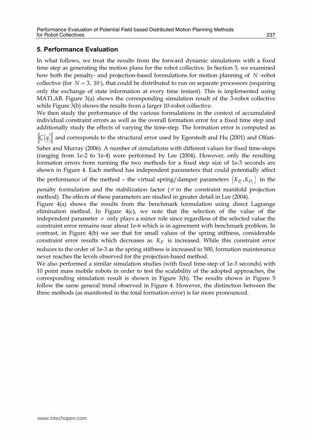
5. Performance Evaluation

In what follows, we treat the results from the forward dynamic simulations with a fixed time step as generating the motion plans for the robot collective. In Section 3, we examined

how both the penalty- and projection-based formulations for motion planning of N -robot

collective (for 3, 10N = ), that could be distributed to run on separate processors (requiring

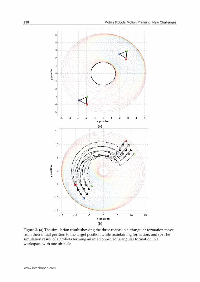
only the exchange of state information at every time instant). This is implemented using MATLAB. Figure 3(a) shows the corresponding simulation result of the 3-robot collective while Figure 3(b) shows the results from a larger 10-robot collective. We then study the performance of the various formulations in the context of accumulated individual constraint errors as well as the overall formation error for a fixed time step and additionally study the effects of varying the time-step. The formation error is computed as

( )C q# #

and corresponds to the structural error used by Egerstedt and Hu (2001) and Olfati-

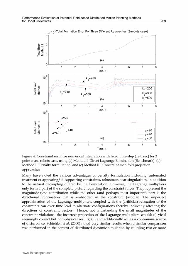
Saber and Murray (2006). A number of simulations with different values for fixed time-steps (ranging from 1e-2 to 1e-4) were performed by Lee (2004). However, only the resulting formation errors from running the two methods for a fixed step size of 1e-3 seconds are shown in Figure 4. Each method has independent parameters that could potentially affect

the performance of the method – the virtual spring/damper parameters ( ),i iP DK K in the

penalty formulation and the stabilization factor (σ in the constraint manifold projection method). The effects of these parameters are studied in greater detail in Lee (2004). Figure 4(a) shows the results from the benchmark formulation using direct Lagrange elimination method. In Figure 4(c), we note that the selection of the value of the independent parameter σ only plays a minor role since regardless of the selected value the constraint error remains near about 1e-6 which is in agreement with benchmark problem. In contrast, in Figure 4(b) we see that for small values of the spring stiffness, considerable

constraint error results which decreases as PK is increased. While this constraint error

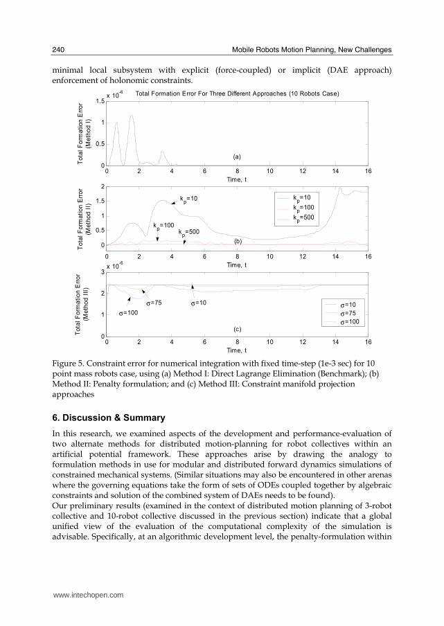
reduces to the order of 1e-3 as the spring stiffness is increased to 500, formation maintenance never reaches the levels observed for the projection-based method. We also performed a similar simulation studies (with fixed time-step of 1e-3 seconds) with 10 point mass mobile robots in order to test the scalability of the adopted approaches, the corresponding simulation result is shown in Figure 3(b). The results shown in Figure 5 follow the same general trend observed in Figure 4. However, the distinction between the three methods (as manifested in the total formation error) is far more pronounced.

www.intechopen.com


238

-5 -4 -3 -2 -1 0 1 2 3 4 5

-5

-4

-3

-2

-1

0

1

2

3

4

5

x position

y p

osit

ion

Simulation of 3 Point Mass Robots

(a)

-15 -10 -5 0 5 10 15

-15

-10

-5

0

5

10

15

x position

y p

osit

ion

(b)

Figure 3. (a) The simulation result showing the three robots in a triangular formation move from their initial position to the target position while maintaining formation; and (b) The simulation result of 10 robots forming an interconnected triangular formation in a workspace with one obstacle

www.intechopen.com


239

0 1 2 3 4 5 6 7 80

1

2

3x 10

-9

To

talE

rro

r

Me

tho

d I

Time, t

Total Formation Error For Three Different Approaches (3-robots case)

0 1 2 3 4 5 6 7 810

-4

10-2

Time, t

To

talE

rro

r

Me

tho

d I

I

kp=200

kp=350

kp=500

0 1 2 3 4 5 6 7 810

-7

10-6

To

talE

rro

r

Me

tho

d I

II

Time, t

σ=20

σ=40

σ=60

σ=40

σ=20

σ=60

kp=200

kp=500

kp=350

(a)

(b)

(c)

Figure 4. Constraint error for numerical integration with fixed time-step (1e-3 sec) for 3 point mass robots case, using (a) Method I: Direct Lagrange Elimination (Benchmark); (b) Method II: Penalty formulation; and (c) Method III: Constraint manifold projection approaches

Many have noted the various advantages of penalty formulation including: automated treatment of appearing/ disappearing constraints, robustness near singularities, in addition to the natural decoupling offered by the formulation. However, the Lagrange multipliers only form a part of the complete picture regarding the constraint forces. They represent the magnitude-type contribution while the other (and perhaps most important) part is the directional information that is embedded in the constraint Jacobian. The imperfect approximation of the Lagrange multipliers, coupled with the (artificial) relaxation of the constraints can over time lead to alternate configurations thereby indirectly affecting the directions of constraint vectors. Hence, not withstanding the small magnitudes of the constraint violations, the incorrect projection of the Lagrange multipliers would: (i) yield seemingly correct but non-physical results; (ii) and additionally act as a continuous source of disturbance. Schiehlen et al. (2000) noted very similar results when a similar comparison was performed in the context of distributed dynamic simulation by coupling two or more

www.intechopen.com


240

minimal local subsystem with explicit (force-coupled) or implicit (DAE approach) enforcement of holonomic constraints.

0 2 4 6 8 10 12 14 160

0.5

1

1.5x 10

-6

To

tal

Fo

rma

tio

n E

rro

r

(Me

tho

d I

)

Time, t

Total Formation Error For Three Different Approaches (10 Robots Case)

0 2 4 6 8 10 12 14 16

0

0.5

1

1.5

2

To

tal

Fo

rma

tio

n E

rro

r

(Me

tho

d I

I)

Time, t

kp=10

kp=100

kp=500

0 2 4 6 8 10 12 14 160

1

2

3x 10

-6

To

tal

Fo

rma

tio

n E

rro

r

(Me

tho

d I

II)

Time, t

σ=10

σ=75

σ=100

(a)

(b)

(c)

kp=10

kp=100

kp=500

σ=10 σ=75

σ=100

Figure 5. Constraint error for numerical integration with fixed time-step (1e-3 sec) for 10 point mass robots case, using (a) Method I: Direct Lagrange Elimination (Benchmark); (b) Method II: Penalty formulation; and (c) Method III: Constraint manifold projection approaches

6. Discussion & Summary

In this research, we examined aspects of the development and performance-evaluation of two alternate methods for distributed motion-planning for robot collectives within an artificial potential framework. These approaches arise by drawing the analogy to formulation methods in use for modular and distributed forward dynamics simulations of constrained mechanical systems. (Similar situations may also be encountered in other arenas where the governing equations take the form of sets of ODEs coupled together by algebraic constraints and solution of the combined system of DAEs needs to be found). Our preliminary results (examined in the context of distributed motion planning of 3-robot collective and 10-robot collective discussed in the previous section) indicate that a global unified view of the evaluation of the computational complexity of the simulation is advisable. Specifically, at an algorithmic development level, the penalty-formulation within

www.intechopen.com


241

an APF framework provides a seemingly natural method for decoupling and distributing the computation, reduced computational complexity and an elegant Lyapunov-based setting to prove stability results. However, this is typically at the cost of formation maintenance – the projection-based approach does not distribute as well and is computationally more expensive per time-step. However, in the overall picture, this approach generates motion plans with smaller formation errors for a specified time-step and would have overall computational advantages over using the penalty formulation with a much smaller time-step.

7. Acknowledgements

We gratefully acknowledge the support from The Research Foundation of State University of New York and National Science Foundation CAREER Award (IIS-0347653) for this research effort.

8. References

Arnold, V. (1989). Mathematical Methods of Classical Mechanics, Springer-Verlag, New York. Ascher, U., Chin, H., Petzold, L. & Reich, S. (1995). Stabilization of Constrained Mechanical

Systems with DAEs and Invariant Manifolds. Mechanical Structures & Machines, Vol.23, 135-158.

Ascher, U., Pai, D. K. & Cloutier, B. (1997). Forward Dynamics, Elimination Methods, and Formulation Stiffness in Robot Simulation. The International Journal of Robotics Research, Vol.16, No.6, 749-758.

Ascher, U. & Petzold, L. (1998). Computer Methods for Ordinary Differential Equations and Differential-Algebraic Equations, SIAM: Society for Industrial and Applied Mathematics, Philadelphia, PA.

Baumgarte, J. (1983). A New Method of Stabilization for Holonomic Constraints. ASME Journal of Applied Mechanics, Vol.50, 869-870.

Beard, R. W., Lawton, J. & Hadaegh, F. Y. (2001). A Feedback Architecture for Formation Control. IEEE Transactions on Control Systems Technology, Vol.9, No.6, 777-790.

Bhatt, R. M., Tang, C. P. & Krovi, V. N. (2008). Formation Optimization for A Fleet of Wheeled Mobile Robots - A Geometric Approach. Robotics and Autonomous Systems. doi:10.1016/j.robot.2006.12.012

Desai, J. P., Ostrowski, J. P. & Kumar, V. (2001). Modeling and Control of Formations of Nonholonomic Mobile Robots. IEEE Transactions on Robotics and Automation, Vol.17, No.6, 905-908.

Egerstedt, M. & Hu, X. (2001). Formation Constrained Multi-Agent Control. IEEE Transactions on Robotics and Automation, Vol.17, No.6, 947-951.

García de Jalón, J. & Bayo, E. (1994). Kinematic and Dynamic Simulation of Multibody Systems: The Real-Time Challenge, Springer-Verlag, New York.

Haug, E. J. (1989). Computer Aided Kinematics and Dynamics of Mechanical Systems: Basic Methods, Allyn and Bacon Series in Engineering, Prentice Hall.

Lawton, J., Beard, R. & Young, B. (2003). A Decentralized Approach To Formation Maneuvers. IEEE Transactions on Robotics and Automation, Vol.19, No.6, 933-941.

www.intechopen.com


242

Lee, L.-F. (2004). Decentralized Motion Planning within an Artificial Potential Framework (APF) For Cooperative Payload Transport by Multi-Robots Collectives. M.S. Thesis. Mechanical and Aerospace Engineering. University at Buffalo, Buffalo, NY.

Leonard, N. E. & Fiorelli, E. (2001). Virtual Leaders, Artificial Potentials and Coordinated Control of Groups, Proceedings of IEEE Conference on Decision and Control, pp. 2968-2973, Orlando, FL.

Lewis, M. A. & Tan, K.-H. (1997). High Precision Formation Control of Mobile Robots Using Virtual Structures. Autonomous Robots, Vol.4, 387-403.

Ogren, P., Egerstedt, M. & Hu., X. (2002). A Control Lyapunov Function Approach to Multi-Agent Coordination. IEEE Transactions on Robotics and Automation, Vol.18, No.5, 847-851.

Olfati-Saber, R. & Murray, R. M. (2002). Graph Rigidity and Distributed Formation Stabilization of Multi-Vehicle Systems, Proceedings of 41st IEEE Conference on Decision and Control, pp. 2965-2971, Las Vegas, Nevada.

Olfati-Saber, R. (2006). Flocking for Multi-Agent Dynamic Systems: Algorithms and Theory. IEEE Transactions on Automatic Control, Vol.51, No.3, 401-420.

Rimon, E. & Koditschek, D. E. (1992). Exact Robot Navigation Using Artificial Potential Functions. Robotics and Automation, IEEE Transactions on, Vol.8, No.5, 501-518.

Schiehlen, W. (1990). Multibody Systems Handbook, Springer-Verlag, Berlin. Schiehlen, W., A., R. & Schirle, T. (2000). Force Coupling Versus Differential Algebraic

Description of Constrained Multibody Systems. Multibody System Dynamics, Vol.4, No.4, 317-340.

Shabana, A. A. (1989). Dynamics of Multibody Systems, Wiley, New York. Wang, P. K. C. (1991). Navigation Strategies for Multiple Autonomous Mobile Robots

Moving in Formation. Journal of Robotic Systems, Vol.8, No.2, 177-195. Young, B., Beard, R. W. & Kelsey, J. M. (2001). A Control Scheme for Improving Multi-

Vehicle Formation Maneuvers, Proceedings of American Control Conference, pp. 704-709, Arlington, VA.

Yun, X. & Sarkar, N. (1998). A Unified Formulation of Robotic Systems with Holonomic and Non Holonomic Constraints. IEEE Transactions on Robotics and Automation, Vol.14, No.4, 640-650.

www.intechopen.com

Motion PlanningEdited by Xing-Jian Jing

ISBN 978-953-7619-01-5Hard cover, 598 pagesPublisher InTechPublished online 01, June, 2008Published in print edition June, 2008

InTech EuropeUniversity Campus STeP Ri Slavka Krautzeka 83/A 51000 Rijeka, Croatia Phone: +385 (51) 770 447 Fax: +385 (51) 686 166www.intechopen.com

InTech ChinaUnit 405, Office Block, Hotel Equatorial Shanghai No.65, Yan An Road (West), Shanghai, 200040, China

Phone: +86-21-62489820 Fax: +86-21-62489821

In this book, new results or developments from different research backgrounds and application fields are puttogether to provide a wide and useful viewpoint on these headed research problems mentioned above,focused on the motion planning problem of mobile ro-bots. These results cover a large range of the problemsthat are frequently encountered in the motion planning of mobile robots both in theoretical methods andpractical applications including obstacle avoidance methods, navigation and localization techniques,environmental modelling or map building methods, and vision signal processing etc. Different methods such aspotential fields, reactive behaviours, neural-fuzzy based methods, motion control methods and so on arestudied. Through this book and its references, the reader will definitely be able to get a thorough overview onthe current research results for this specific topic in robotics. The book is intended for the readers who areinterested and active in the field of robotics and especially for those who want to study and develop their ownmethods in motion/path planning or control for an intelligent robotic system.

How to referenceIn order to correctly reference this scholarly work, feel free to copy and paste the following:

Leng-Feng Lee and Venkat N. Krovi (2008). Performance Evaluation of Potential Field Based DistributedMotion Planning Methods for Robot Collectives, Motion Planning, Xing-Jian Jing (Ed.), ISBN: 978-953-7619-01-5, InTech, Available from:http://www.intechopen.com/books/motion_planning/performance_evaluation_of_potential_field_based_distributed_motion_planning_methods_for_robot_collec

© 2008 The Author(s). Licensee IntechOpen. This chapter is distributedunder the terms of the Creative Commons Attribution-NonCommercial-ShareAlike-3.0 License, which permits use, distribution and reproduction fornon-commercial purposes, provided the original is properly cited andderivative works building on this content are distributed under the samelicense.

https://creativecommons.org/licenses/by-nc-sa/3.0/

Documents

12 - IntechOpen