12 Monopolistic Competition and Oligopolypioneer.netserv.chula.ac.th/~achairat/12_Monopolistic... · · 2017-04-1812.2 Oligopoly 12.3 Price Competition ... 11. 1. Suppose all firms

12 Monopolistic Competition and

Oligopoly

Read Pindyck and Rubinfeld (2012), Chapter 12

•Chapter 12 Monopolistic Competition and Oligopoly .. Economics I: 2900111 . Chairat Aemkulwat 4/18/2017

CHAPTER 12 OUTLINE

12.1 Monopolistic Competition

12.2 Oligopoly

12.3 Price Competition

12.4 Competition versus Collusion:

The Prisoners’ Dilemma

12.5 Implications of the Prisoners’ Dilemma for

Oligopolistic Pricing

12.6 Cartels

•Chapter 12 Monopolistic Competition and Oligopoly .. Economics I: 2900111 . Chairat Aemkulwat

Monopolistic Competition and Oligopoly

● monopolistic competition Market in which firms can

enter freely, each producing its own brand or version of a

differentiated product.

● oligopoly Market in which only a few firms compete

with one another, and entry by new firms is impeded.

● cartel Market in which some or all firms explicitly

collude, coordinating prices and output levels to

maximize joint profits.

•Chapter 12 Monopolistic Competition and Oligopoly .. Economics I: 2900111 . Chairat Aemkulwat3

MONOPOLISTIC COMPETITION12.1

The Makings of Monopolistic Competition

A monopolistically competitive market has two key characteristics:

1. Firms compete by selling differentiated products that are highly

substitutable for one another but not perfect substitutes. In other

words, the cross-price elasticities of demand are large but not

infinite.

2. There is free entry and exit: it is relatively easy for new firms to

enter the market with their own brands and for existing firms to

leave if their products become unprofitable.



Equilibrium in the Short Run and the Long Run

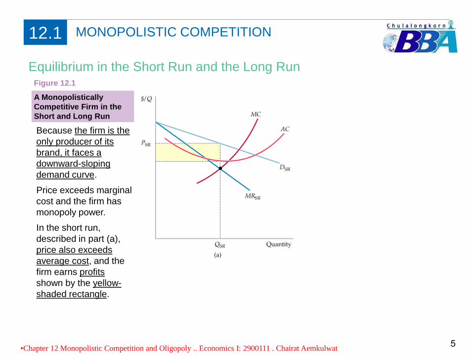
Because the firm is the

only producer of its

brand, it faces a

downward-sloping

demand curve.

Price exceeds marginal

cost and the firm has

monopoly power.

In the short run,

described in part (a),

price also exceeds

average cost, and the

firm earns profits

shown by the yellow-

shaded rectangle.

A Monopolistically

Competitive Firm in the

Short and Long Run

Figure 12.1



Equilibrium in the Short Run and the Long Run

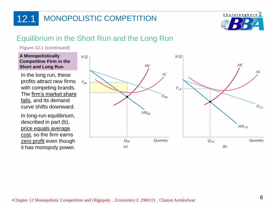
In the long run, these

profits attract new firms

with competing brands.

The firm’s market share

falls, and its demand

curve shifts downward.

In long-run equilibrium,

described in part (b),

price equals average

cost, so the firm earns

zero profit even though

it has monopoly power.

A Monopolistically

Competitive Firm in the

Short and Long Run

Figure 12.1 (continued)



Monopolistic Competition and Economic Efficiency

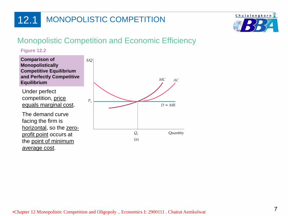
Under perfect

competition, price

equals marginal cost.

The demand curve

facing the firm is

horizontal, so the zero-

profit point occurs at

the point of minimum

average cost.

Comparison of

Monopolistically

Competitive Equilibrium

and Perfectly Competitive

Equilibrium

Figure 12.2


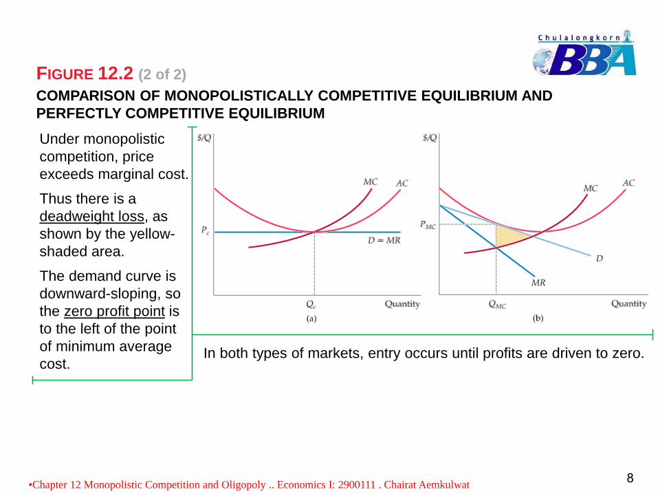
COMPARISON OF MONOPOLISTICALLY COMPETITIVE EQUILIBRIUM AND

PERFECTLY COMPETITIVE EQUILIBRIUM

FIGURE 12.2 (2 of 2)

Under monopolistic

competition, price

exceeds marginal cost.

Thus there is a

deadweight loss, as

shown by the yellow-

shaded area.

The demand curve is

downward-sloping, so

the zero profit point is

to the left of the point

of minimum average

cost.In both types of markets, entry occurs until profits are driven to zero.


Is monopolistic competition then a socially undesirable market structure

that should be regulated? The answer—for two reasons—is probably no:

1. In most monopolistically competitive markets, monopoly power is small.

Usually enough firms compete, with brands that are sufficiently substitutable,

so that no single firm has much monopoly power. Any resulting deadweight

loss will therefore be small. And because firms’ demand curves will be fairly

elastic, average cost will be close to the minimum.

2. Any inefficiency must be balanced against an important benefit from

monopolistic competition: product diversity.

Most consumers value the ability to choose among a wide variety of

competing products and brands that differ in various ways. The gains from

product diversity can be large and may easily outweigh the inefficiency costs

resulting from downward-sloping demand curves.


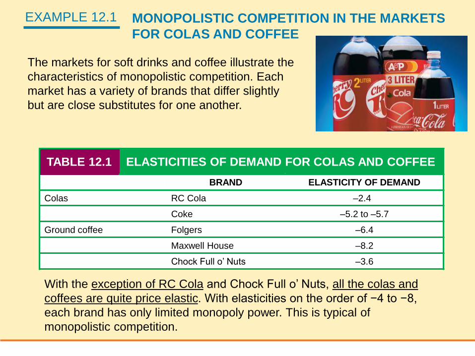
EXAMPLE 12.1 MONOPOLISTIC COMPETITION IN THE MARKETS

FOR COLAS AND COFFEE

TABLE 12.1 ELASTICITIES OF DEMAND FOR COLAS AND COFFEE

BRAND ELASTICITY OF DEMAND

Colas RC Cola –2.4

Coke –5.2 to –5.7

Ground coffee Folgers –6.4

Maxwell House –8.2

Chock Full o’ Nuts –3.6

With the exception of RC Cola and Chock Full o’ Nuts, all the colas and

coffees are quite price elastic. With elasticities on the order of −4 to −8,

each brand has only limited monopoly power. This is typical of

monopolistic competition.

The markets for soft drinks and coffee illustrate the

characteristics of monopolistic competition. Each

market has a variety of brands that differ slightly

but are close substitutes for one another.

1. Suppose all firms in a monopolistically

competitive industry were merged into one

large firm. Would that new firm produce as

many different brands? Would it produce only

a single brand? Explain.


1. Suppose all firms in a monopolistically competitive

industry were merged into one large firm. Would that

new firm produce as many different brands? Would it

produce only a single brand? Explain.


• Monopolistic competition is defined by product differentiation.

Each firm earns economic profit by distinguishing its brand from

all other brands. This distinction can arise from underlying

differences in the product or from differences in advertising.

• If these competitors merge into a single firm, the resulting

monopolist would not produce as many brands, since too much

brand competition is internecine (mutually destructive). However,

it is unlikely that only one brand would be produced after the

merger.

• Producing several brands with different prices and characteristics

is one method of splitting the market into sets of customers with

different price elasticities. The monopolist can sell to more

consumers and maximize overall profit by producing multiplebrands and practicing a form of price discrimination.

ANS.

In oligopolistic markets, the products may or may not be differentiated.

What matters is that only a few firms account for most or all of total production.

• In some oligopolistic markets, some or all firms earn substantial profits over the

long run because barriers to entry make it difficult or impossible for new firms to

enter.

• Examples of oligopolistic industries include automobiles, steel, aluminum,

petrochemicals, electrical equipment, and computers.

Oligopoly is a prevalent form of market structure.

• Scale economies may make it unprofitable for more than a few firms to coexist in

the market;

• patents or access to a technology may exclude potential competitors; and

• the need to spend money for name recognition and market reputation may

discourage entry by new firms. These are “natural” entry barriers—they are basic

to the structure of the particular market. In addition, incumbent firms may take

strategic actions to deter entry.

Managing an oligopolistic firm is complicated because pricing, output,

advertising, and investment decisions involve important strategic

considerations, which can be highly complex.

Oligopoly12.2


Equilibrium in an Oligopolistic Market

In an oligopolistic market, however, a firm sets price or output based partly on

strategic considerations regarding the behavior of its competitors.

With some modification, the underlying principle to describe an equilibrium

when firms make decisions that explicitly take each other’s behavior into

account is the same as the equilibrium in competitive and monopolistic

markets: When a market is in equilibrium, firms are doing the best they can and

have no reason to change their price or output.

NASH EQUILIBRIUM

● Nash equilibrium Set of strategies or actions in which each firm does the

best it can given its competitors’ actions.

● duopoly Market in which two firms compete with each other.

Nash Equilibrium: Each firm is doing the best it can given what its competitors

are doing.


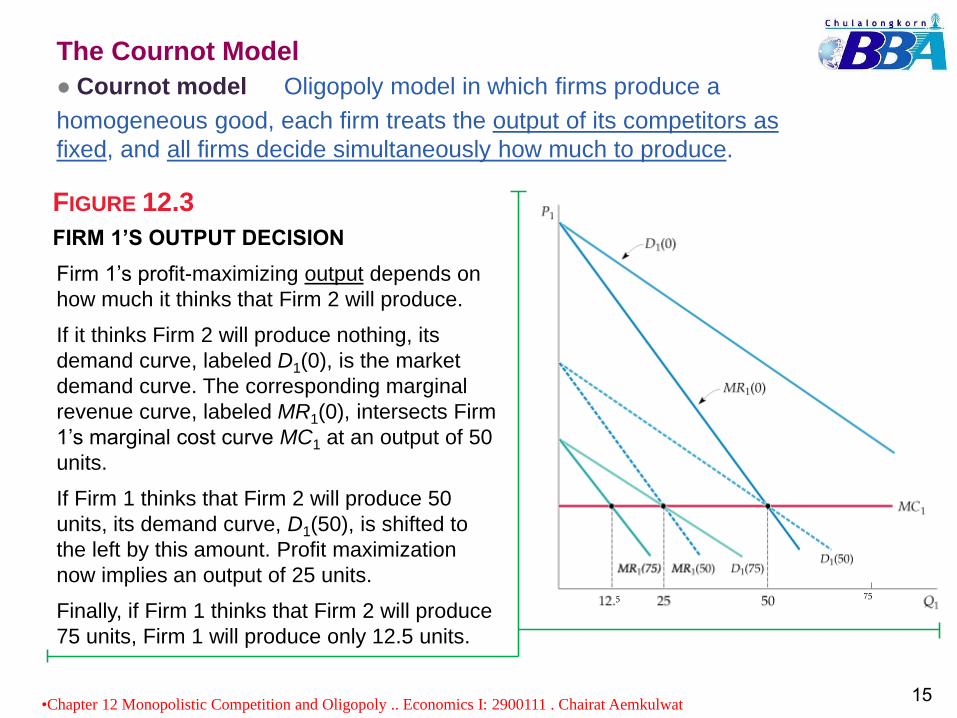
FIRM 1’S OUTPUT DECISION

FIGURE 12.3

The Cournot Model

● Cournot model Oligopoly model in which firms produce a

homogeneous good, each firm treats the output of its competitors as

fixed, and all firms decide simultaneously how much to produce.

Firm 1’s profit-maximizing output depends on

how much it thinks that Firm 2 will produce.

If it thinks Firm 2 will produce nothing, its

demand curve, labeled D1(0), is the market

demand curve. The corresponding marginal

revenue curve, labeled MR1(0), intersects Firm

1’s marginal cost curve MC1 at an output of 50

units.

If Firm 1 thinks that Firm 2 will produce 50

units, its demand curve, D1(50), is shifted to

the left by this amount. Profit maximization

now implies an output of 25 units.

Finally, if Firm 1 thinks that Firm 2 will produce

75 units, Firm 1 will produce only 12.5 units.

5 75


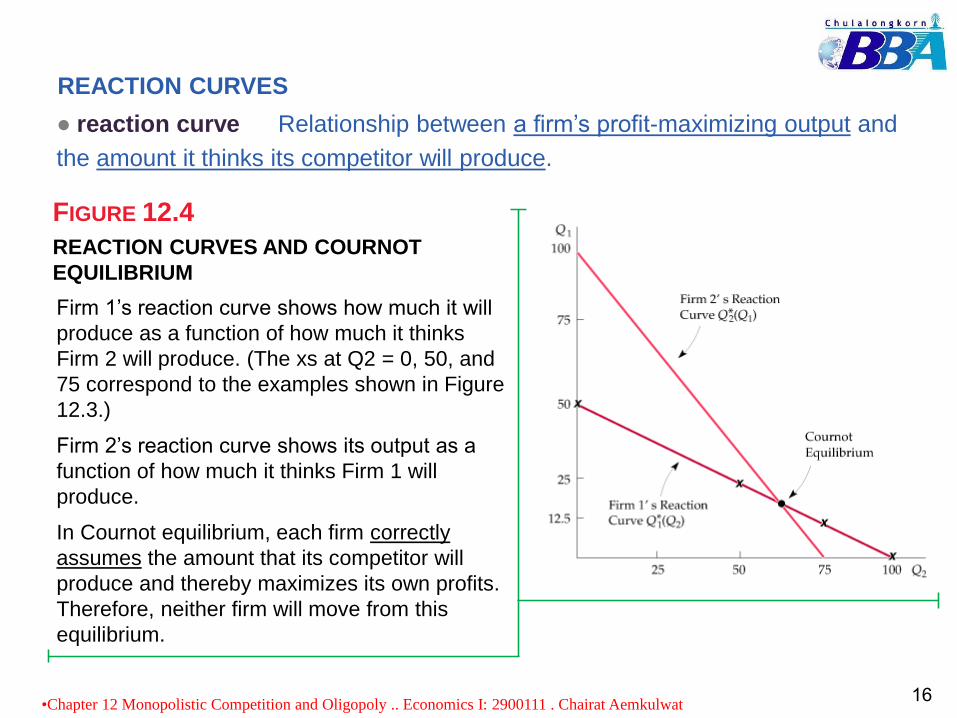
REACTION CURVES AND COURNOT

EQUILIBRIUM

FIGURE 12.4

● reaction curve Relationship between a firm’s profit-maximizing output and

the amount it thinks its competitor will produce.

Firm 1’s reaction curve shows how much it will

produce as a function of how much it thinks

Firm 2 will produce. (The xs at Q2 = 0, 50, and

75 correspond to the examples shown in Figure

12.3.)

Firm 2’s reaction curve shows its output as a

function of how much it thinks Firm 1 will

produce.

In Cournot equilibrium, each firm correctly

assumes the amount that its competitor will

produce and thereby maximizes its own profits.

Therefore, neither firm will move from this

equilibrium.

REACTION CURVES


● Cournot equilibrium Equilibrium in the Cournot model in which each firm

correctly assumes how much its competitor will produce and sets its own

production level accordingly.

COURNOT EQUILIBRIUM

Cournot equilibrium is an example of a Nash equilibrium (and thus it is

sometimes called a Cournot-Nash equilibrium).

In a Nash equilibrium, each firm is doing the best it can given what its

competitors are doing.

As a result, no firm would individually want to change its behavior. In the

Cournot equilibrium, each firm is producing an amount that maximizes its profit

given what its competitor is producing, so neither would want to change its

output.


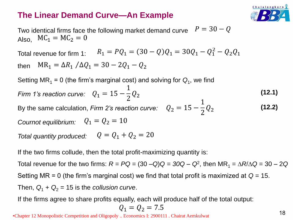
The Linear Demand Curve—An Example

Two identical firms face the following market demand curve

Also,

Total revenue for firm 1:

then

Setting MR1 = 0 (the firm’s marginal cost) and solving for Q1, we find

Firm 1’s reaction curve:

By the same calculation, Firm 2’s reaction curve:

Cournot equilibrium:

Total quantity produced:

If the two firms collude, then the total profit-maximizing quantity is:

Total revenue for the two firms: R = PQ = (30 –Q)Q = 30Q – Q2, then MR1 = ∆R/∆Q = 30 – 2Q

Setting MR = 0 (the firm’s marginal cost) we find that total profit is maximized at Q = 15.

Then, Q1 + Q2 = 15 is the collusion curve.

If the firms agree to share profits equally, each will produce half of the total output:

(12.1)

(12.2)


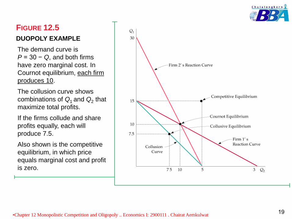
DUOPOLY EXAMPLE

FIGURE 12.5

The demand curve is

P = 30 − Q, and both firms

have zero marginal cost. In

Cournot equilibrium, each firm

produces 10.

The collusion curve shows

combinations of Q1 and Q2 that

maximize total profits.

If the firms collude and share

profits equally, each will

produce 7.5.

Also shown is the competitive

equilibrium, in which price

equals marginal cost and profit

is zero.


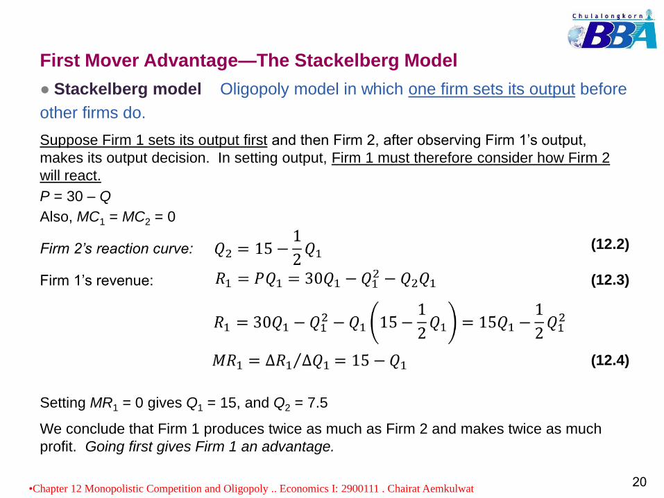
First Mover Advantage—The Stackelberg Model

● Stackelberg model Oligopoly model in which one firm sets its output before

other firms do.

Suppose Firm 1 sets its output first and then Firm 2, after observing Firm 1’s output,

makes its output decision. In setting output, Firm 1 must therefore consider how Firm 2

will react.

P = 30 – Q

Also, MC1 = MC2 = 0


Firm 1’s revenue:

Setting MR1 = 0 gives Q1 = 15, and Q2 = 7.5

We conclude that Firm 1 produces twice as much as Firm 2 and makes twice as much

profit. Going first gives Firm 1 an advantage.

(12.2)

(12.3)

(12.4)


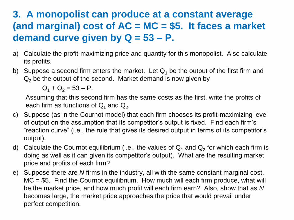
3. A monopolist can produce at a constant average

(and marginal) cost of AC = MC = $5. It faces a market

demand curve given by Q = 53 – P.

a) Calculate the profit-maximizing price and quantity for this monopolist. Also calculate

its profits.

b) Suppose a second firm enters the market. Let Q1 be the output of the first firm and

Q2 be the output of the second. Market demand is now given by

Q1 + Q2 = 53 – P.

Assuming that this second firm has the same costs as the first, write the profits of

each firm as functions of Q1 and Q2.

c) Suppose (as in the Cournot model) that each firm chooses its profit-maximizing level

of output on the assumption that its competitor’s output is fixed. Find each firm’s

“reaction curve” (i.e., the rule that gives its desired output in terms of its competitor’s

output).

d) Calculate the Cournot equilibrium (i.e., the values of Q1 and Q2 for which each firm is

doing as well as it can given its competitor’s output). What are the resulting market

price and profits of each firm?

e) Suppose there are N firms in the industry, all with the same constant marginal cost,

MC = $5. Find the Cournot equilibrium. How much will each firm produce, what will

be the market price, and how much profit will each firm earn? Also, show that as N

becomes large, the market price approaches the price that would prevail under

perfect competition.

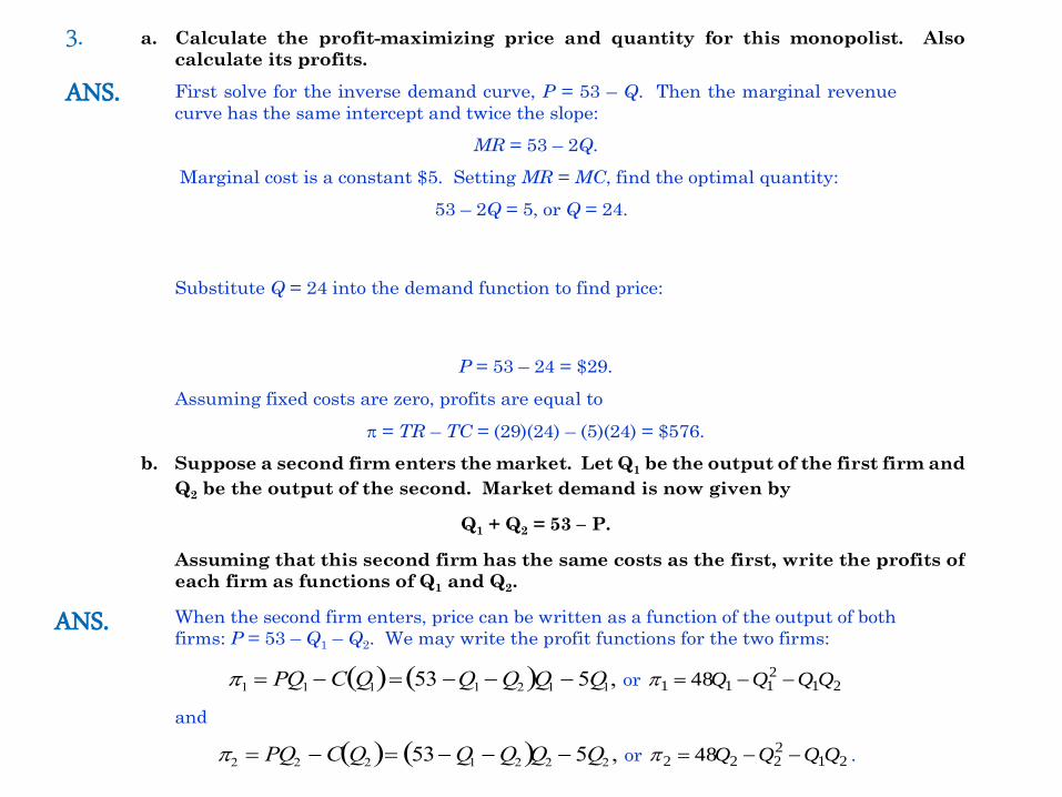
a. Calculate the profit-maximizing price and quantity for this monopolist. Also

calculate its profits.

First solve for the inverse demand curve, P = 53 – Q. Then the marginal revenue

curve has the same intercept and twice the slope:

MR = 53 – 2Q.

Marginal cost is a constant $5. Setting MR = MC, find the optimal quantity:

53 – 2Q = 5, or Q = 24.

Substitute Q = 24 into the demand function to find price:

P = 53 – 24 = $29.

Assuming fixed costs are zero, profits are equal to

= TR – TC = (29)(24) – (5)(24) = $576.

b. Suppose a second firm enters the market. Let Q1 be the output of the first firm and


Q1 + Q2 = 53 – P.



When the second firm enters, price can be written as a function of the output of both

firms: P = 53 – Q1 – Q2. We may write the profit functions for the two firms:

1 PQ1 C Q1 53 Q1 Q2 Q1 5Q1, or 212111 48 QQQQ

and

2 PQ2 C Q2 53Q1 Q2 Q2 5Q2 , or 212222 48 QQQQ .

3. ANS.

ANS.

a. Calculate the profit-maximizing price and quantity for this monopolist. Also

calculate its profits.

First solve for the inverse demand curve, P = 53 – Q. Then the marginal revenue

curve has the same intercept and twice the slope:

MR = 53 – 2Q.

Marginal cost is a constant $5. Setting MR = MC, find the optimal quantity:

53 – 2Q = 5, or Q = 24.

Substitute Q = 24 into the demand function to find price:

P = 53 – 24 = $29.

Assuming fixed costs are zero, profits are equal to

= TR – TC = (29)(24) – (5)(24) = $576.

b. Suppose a second firm enters the market. Let Q1 be the output of the first firm and


Q1 + Q2 = 53 – P.



When the second firm enters, price can be written as a function of the output of both

firms: P = 53 – Q1 – Q2. We may write the profit functions for the two firms:

1 PQ1 C Q1 53 Q1 Q2 Q1 5Q1, or 212111 48 QQQQ

and

2 PQ2 C Q2 53Q1 Q2 Q2 5Q2 , or 212222 48 QQQQ .

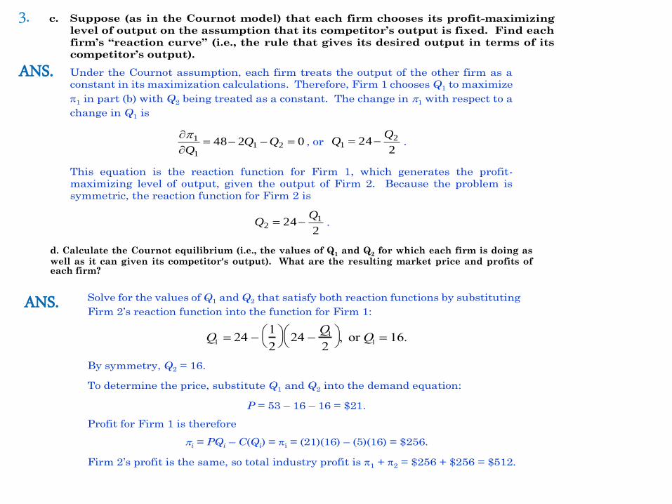
c. Suppose (as in the Cournot model) that each firm chooses its profit-maximizing

level of output on the assumption that its competitor’s output is fixed. Find each

firm’s “reaction curve” (i.e., the rule that gives its desired output in terms of its

competitor’s output).

Under the Cournot assumption, each firm treats the output of the other firm as a

constant in its maximization calculations. Therefore, Firm 1 chooses Q1 to maximize

1 in part (b) with Q2 being treated as a constant. The change in 1 with respect to a

change in Q1 is

0248 211

1

QQ

Q

, or

224 2

1

QQ .

This equation is the reaction function for Firm 1, which generates the profit-

maximizing level of output, given the output of Firm 2. Because the problem is

symmetric, the reaction function for Firm 2 is

224 1

2

QQ .

Solve for the values of Q1 and Q2 that satisfy both reaction functions by substituting

Firm 2’s reaction function into the function for Firm 1:

Q1 24 1

2

24 Q1

2

, or Q1 16.

By symmetry, Q2 = 16.

To determine the price, substitute Q1 and Q2 into the demand equation:

P = 53 – 16 – 16 = $21.

Profit for Firm 1 is therefore

i = PQi – C(Qi) = i = (21)(16) – (5)(16) = $256.

Firm 2’s profit is the same, so total industry profit is 1 + 2 = $256 + $256 = $512.

d. Calculate the Cournot equilibrium (i.e., the values of Q1 and Q2 for which each firm is doing aswell as it can given its competitor’s output). What are the resulting market price and profits ofeach firm?

3.

ANS.

ANS.

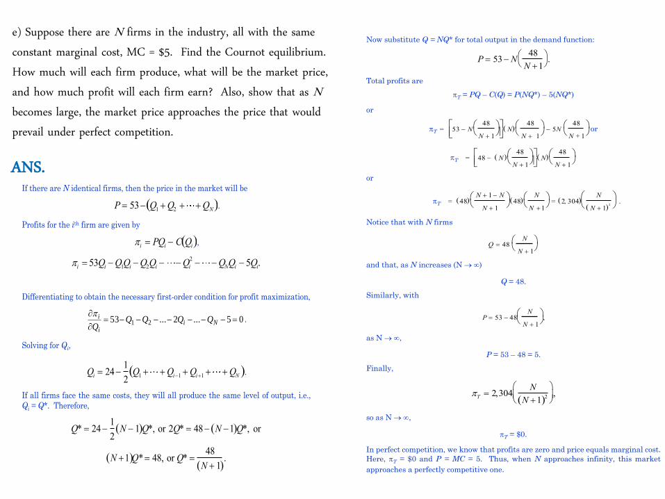
If there are N identical firms, then the price in the market will be

P 53 Q1 Q2 QN .

Profits for the ith firm are given by

i PQi C Qi ,

i 53Qi Q1Qi Q2Qi Qi

2 QNQi 5Qi.

Differentiating to obtain the necessary first-order condition for profit maximization,

05...2...53 21

Ni

i

i QQQQQ

.

Solving for Qi,

Qi 241

2Q1 Qi1 Qi1 QN .

If all firms face the same costs, they will all produce the same level of output, i.e.,

Qi = Q*. Therefore,

Q* 241

2N 1 Q*, or 2Q* 48 N 1 Q*, or

N 1 Q* 48, or Q* 48

N 1 .

Now substitute Q = NQ* for total output in the demand function:

P 53N48

N 1

.

Total profits are

T = PQ – C(Q) = P(NQ*) – 5(NQ*)

or

T = 53 N48

N 1

N 48

N 1

5N

48

N +1

or

T = 48 N 48

N 1

N 48

N 1

or

T = 48 N 1 N

N 1

48

N

N 1

= 2, 304

N

N 1 2

.

Notice that with N firms

Q 48 N

N 1

and that, as N increases (N )

Q = 48.

Similarly, with

P 53 48N

N 1

,

as N ,

P = 53 – 48 = 5.

Finally,

T 2,304N

N 1 2

,

so as N ,

T = $0.

In perfect competition, we know that profits are zero and price equals marginal cost.

Here, T = $0 and P = MC = 5. Thus, when N approaches infinity, this market

approaches a perfectly competitive one.

e) Suppose there are N firms in the industry, all with the same constant marginal cost, MC = $5. Find the Cournot equilibrium. How much will each firm produce, what will be the market price, and how much profit will each firm earn? Also, show that as Nbecomes large, the market price approaches the price that would prevail under perfect competition.

ANS.

5. Two firms compete in selling identical widgets. They choose

their output levels Q1 and Q2 simultaneously and face the demand

curve

P = 30 – Q

where Q = Q1 + Q2. Until recently, both firms had zero marginal

costs. Recent environmental regulations have increased Firm 2’s

marginal cost to $15. Firm 1’s marginal cost remains constant at

zero. True or false: As a result, the market price will rise to the

monopoly level.


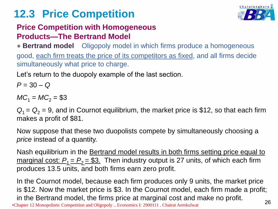
Price Competition12.3Price Competition with Homogeneous

Products—The Bertrand Model● Bertrand model Oligopoly model in which firms produce a homogeneous

good, each firm treats the price of its competitors as fixed, and all firms decide

simultaneously what price to charge.

Let’s return to the duopoly example of the last section.

P = 30 – Q

MC1 = MC2 = $3

Q1 = Q2 = 9, and in Cournot equilibrium, the market price is $12, so that each firm

makes a profit of $81.

Now suppose that these two duopolists compete by simultaneously choosing a

price instead of a quantity.

Nash equilibrium in the Bertrand model results in both firms setting price equal to

marginal cost: P1 = P2 = $3. Then industry output is 27 units, of which each firm

produces 13.5 units, and both firms earn zero profit.

In the Cournot model, because each firm produces only 9 units, the market price

is $12. Now the market price is $3. In the Cournot model, each firm made a profit;

in the Bertrand model, the firms price at marginal cost and make no profit.•Chapter 12 Monopolistic Competition and Oligopoly .. Economics I: 2900111 . Chairat Aemkulwat

26

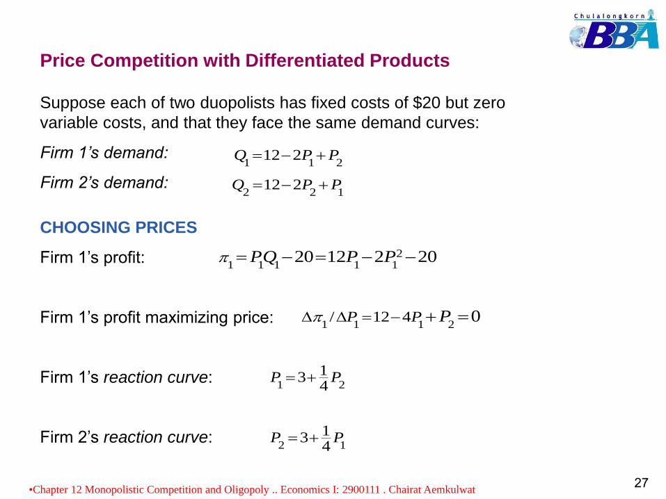
Price Competition with Differentiated Products

Suppose each of two duopolists has fixed costs of $20 but zero

variable costs, and that they face the same demand curves:

Firm 1’s demand:

Firm 2’s demand:

CHOOSING PRICES

Firm 1’s profit:

Firm 1’s profit maximizing price:



1 1 212 2Q P P

2 2 112 2Q P P

1 2

13

4P P

21 1 1 1 1

20 12 2 20PQ P P

1 1 1 2/ 12 4 0P P P

2 1

13

4P P


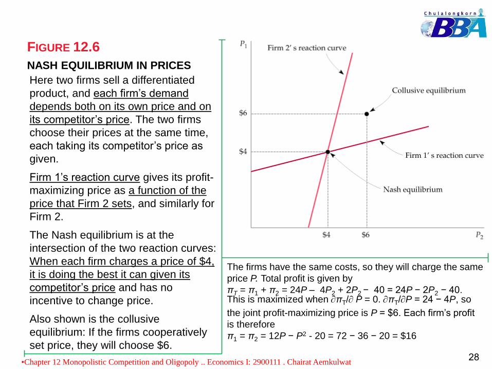
NASH EQUILIBRIUM IN PRICES

FIGURE 12.6

Here two firms sell a differentiated

product, and each firm’s demand

depends both on its own price and on

its competitor’s price. The two firms

choose their prices at the same time,

each taking its competitor’s price as

given.

Firm 1’s reaction curve gives its profit-

maximizing price as a function of the

price that Firm 2 sets, and similarly for

Firm 2.

The Nash equilibrium is at the

intersection of the two reaction curves:

When each firm charges a price of $4,

it is doing the best it can given its

competitor’s price and has no

incentive to change price.

Also shown is the collusive

equilibrium: If the firms cooperatively

set price, they will choose $6.

The firms have the same costs, so they will charge the same

price P. Total profit is given by

πT = π1 + π2 = 24P – 4P2 + 2P2 − 40 = 24P − 2P2 − 40.This is maximized when πT/ P = 0. πT/P = 24 − 4P, so

the joint profit-maximizing price is P = $6. Each firm’s profit

is therefore

π1 = π2 = 12P − P2 - 20 = 72 − 36 − 20 = $16


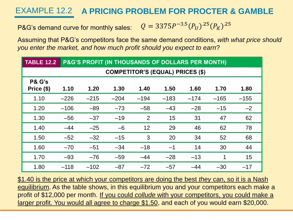
EXAMPLE 12.2 A PRICING PROBLEM FOR PROCTER & GAMBLE

P&G’s demand curve for monthly sales:

Assuming that P&G’s competitors face the same demand conditions, with what price should

you enter the market, and how much profit should you expect to earn?

TABLE 12.2 P&G’S PROFIT (IN THOUSANDS OF DOLLARS PER MONTH)

COMPETITOR’S (EQUAL) PRICES ($)

P& G’s

Price ($) 1.10 1.20 1.30 1.40 1.50 1.60 1.70 1.80

1.10 –226 –215 –204 –194 –183 –174 –165 –155

1.20 –106 –89 –73 –58 –43 –28 –15 –2

1.30 –56 –37 –19 2 15 31 47 62

1.40 –44 –25 –6 12 29 46 62 78

1.50 –52 –32 –15 3 20 34 52 68

1.60 –70 –51 –34 –18 –1 14 30 44

1.70 –93 –76 –59 –44 –28 –13 1 15

1.80 –118 –102 –87 –72 –57 –44 –30 –17

$1.40 is the price at which your competitors are doing the best they can, so it is a Nash

equilibrium. As the table shows, in this equilibrium you and your competitors each make a

profit of $12,000 per month. If you could collude with your competitors, you could make a

larger profit. You would all agree to charge $1.50, and each of you would earn $20,000.

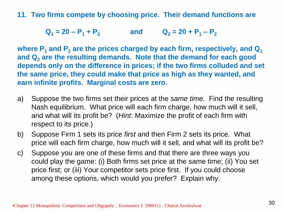
11. Two firms compete by choosing price. Their demand functions are

Q1 = 20 – P1 + P2 and Q2 = 20 + P1 – P2

where P1 and P2 are the prices charged by each firm, respectively, and Q1

and Q2 are the resulting demands. Note that the demand for each good

depends only on the difference in prices; if the two firms colluded and set

the same price, they could make that price as high as they wanted, and

earn infinite profits. Marginal costs are zero.

a) Suppose the two firms set their prices at the same time. Find the resulting

Nash equilibrium. What price will each firm charge, how much will it sell,

and what will its profit be? (Hint: Maximize the profit of each firm with

respect to its price.)

b) Suppose Firm 1 sets its price first and then Firm 2 sets its price. What

price will each firm charge, how much will it sell, and what will its profit be?

c) Suppose you are one of these firms and that there are three ways you

could play the game: (i) Both firms set price at the same time; (ii) You set

price first; or (iii) Your competitor sets price first. If you could choose

among these options, which would you prefer? Explain why.


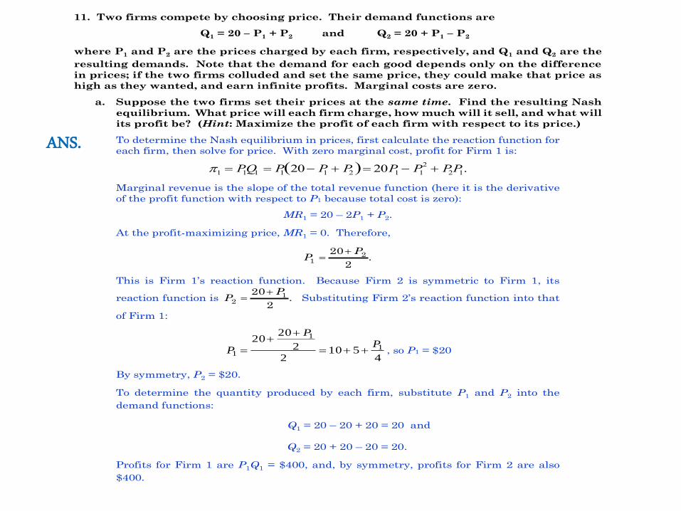
11. Two firms compete by choosing price. Their demand functions are

Q1 = 20 – P1 + P2 and Q2 = 20 + P1 – P2

where P1 and P2 are the prices charged by each firm, respectively, and Q1 and Q2 are the

resulting demands. Note that the demand for each good depends only on the difference

in prices; if the two firms colluded and set the same price, they could make that price as

high as they wanted, and earn infinite profits. Marginal costs are zero.

a. Suppose the two firms set their prices at the same time. Find the resulting Nash

equilibrium. What price will each firm charge, how much will it sell, and what will

its profit be? (Hint: Maximize the profit of each firm with respect to its price.)

To determine the Nash equilibrium in prices, first calculate the reaction function for

each firm, then solve for price. With zero marginal cost, profit for Firm 1 is:

1 P1Q1 P1 20 P1 P2 20P1 P1

2 P2P1.

Marginal revenue is the slope of the total revenue function (here it is the derivative

of the profit function with respect to P1 because total cost is zero):

MR1 = 20 – 2P1 + P2.

At the profit-maximizing price, MR1 = 0. Therefore,

PP

1220

2

.

This is Firm 1’s reaction function. Because Firm 2 is symmetric to Firm 1, its

reaction function is PP

2120

2

. Substituting Firm 2’s reaction function into that

of Firm 1:

4510

2

2

2020

1

1

1

P

P

P

, so P1 = $20

By symmetry, P2 = $20.

To determine the quantity produced by each firm, substitute P1 and P2 into the

demand functions:

Q1 = 20 – 20 + 20 = 20 and

Q2 = 20 + 20 – 20 = 20.

Profits for Firm 1 are P1Q1 = $400, and, by symmetry, profits for Firm 2 are also

$400.

ANS.

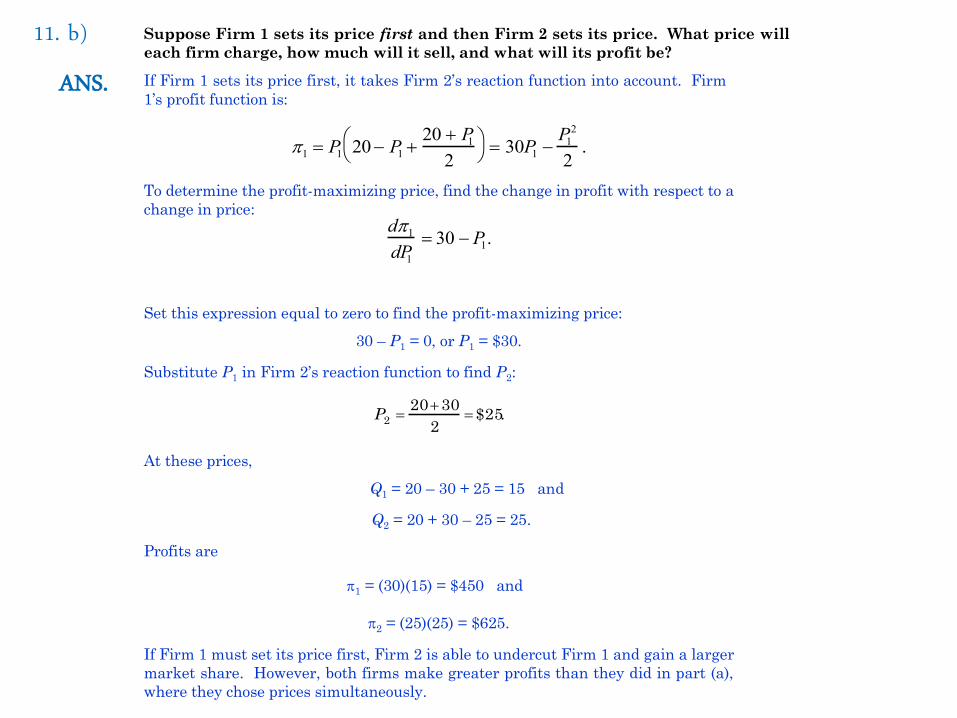
Suppose Firm 1 sets its price first and then Firm 2 sets its price. What price will

each firm charge, how much will it sell, and what will its profit be?

If Firm 1 sets its price first, it takes Firm 2’s reaction function into account. Firm

1’s profit function is:

1 P1 20 P1 20 P1

2

30P1

P1

2

2.

To determine the profit-maximizing price, find the change in profit with respect to a

change in price: d1

dP1

30 P1.

Set this expression equal to zero to find the profit-maximizing price:

30 – P1 = 0, or P1 = $30.

Substitute P1 in Firm 2’s reaction function to find P2:

P2

20 30

2

$25.

At these prices,

Q1 = 20 – 30 + 25 = 15 and

Q2 = 20 + 30 – 25 = 25.

Profits are

1 = (30)(15) = $450 and

2 = (25)(25) = $625.

If Firm 1 must set its price first, Firm 2 is able to undercut Firm 1 and gain a larger

market share. However, both firms make greater profits than they did in part (a),

where they chose prices simultaneously.

11. b) ANS.

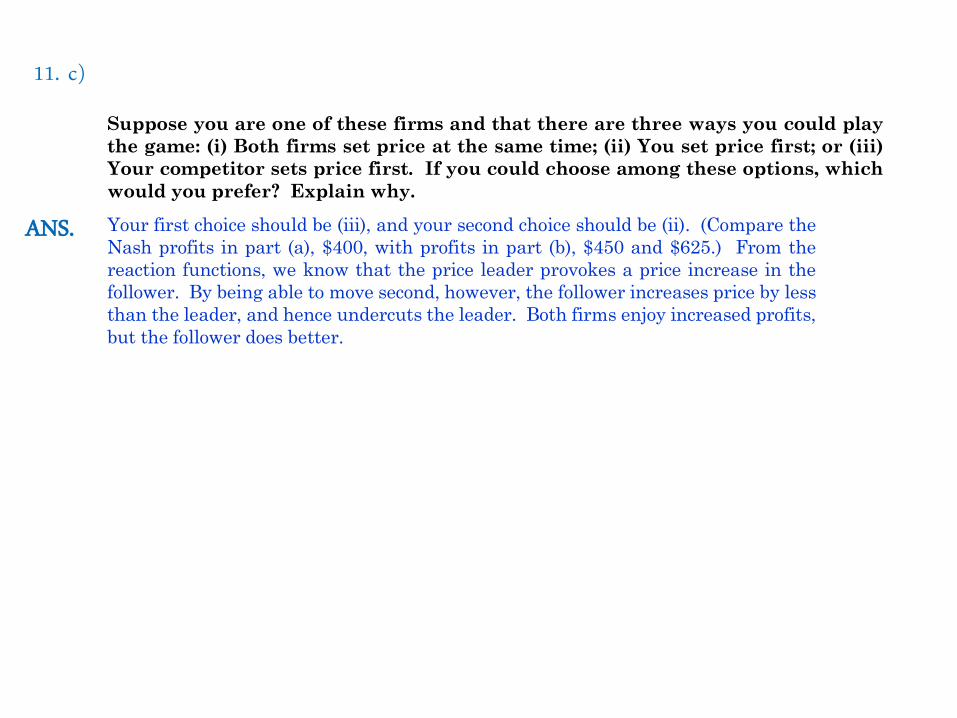
Suppose you are one of these firms and that there are three ways you could play

the game: (i) Both firms set price at the same time; (ii) You set price first; or (iii)

Your competitor sets price first. If you could choose among these options, which

would you prefer? Explain why.

Your first choice should be (iii), and your second choice should be (ii). (Compare the

Nash profits in part (a), $400, with profits in part (b), $450 and $625.) From the

reaction functions, we know that the price leader provokes a price increase in the

follower. By being able to move second, however, the follower increases price by less

than the leader, and hence undercuts the leader. Both firms enjoy increased profits,

but the follower does better.

11. c)

ANS.

7. Suppose that two competing firms, A and B,

produce a homogeneous good. Both firms have a

marginal cost of MC = $50. Describe what would

happen to output and price in each of the following

situations if the firms are at (i) Cournot equilibrium, (ii)

collusive equilibrium, and (iii) Bertrand equilibrium.

1. Because Firm A must increase wages, its MC

increases to $80.

2. The marginal cost of both firms increases.

3. The demand curve shifts to the right.


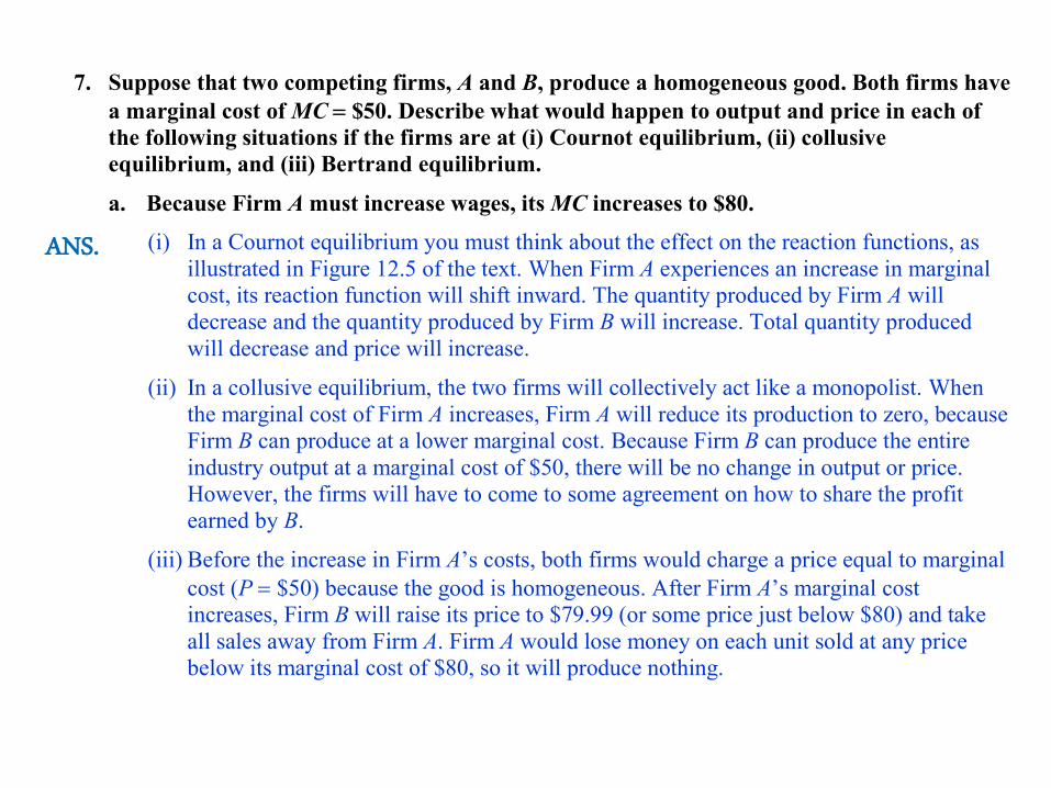
7. Suppose that two competing firms, A and B, produce a homogeneous good. Both firms have

a marginal cost of MC $50. Describe what would happen to output and price in each of

the following situations if the firms are at (i) Cournot equilibrium, (ii) collusive

equilibrium, and (iii) Bertrand equilibrium.

a. Because Firm A must increase wages, its MC increases to $80.

(i) In a Cournot equilibrium you must think about the effect on the reaction functions, as

illustrated in Figure 12.5 of the text. When Firm A experiences an increase in marginal

cost, its reaction function will shift inward. The quantity produced by Firm A will

decrease and the quantity produced by Firm B will increase. Total quantity produced

will decrease and price will increase.

(ii) In a collusive equilibrium, the two firms will collectively act like a monopolist. When

the marginal cost of Firm A increases, Firm A will reduce its production to zero, because

Firm B can produce at a lower marginal cost. Because Firm B can produce the entire

industry output at a marginal cost of $50, there will be no change in output or price.

However, the firms will have to come to some agreement on how to share the profit

earned by B.

(iii) Before the increase in Firm A’s costs, both firms would charge a price equal to marginal

cost (P $50) because the good is homogeneous. After Firm A’s marginal cost

increases, Firm B will raise its price to $79.99 (or some price just below $80) and take

all sales away from Firm A. Firm A would lose money on each unit sold at any price

below its marginal cost of $80, so it will produce nothing.

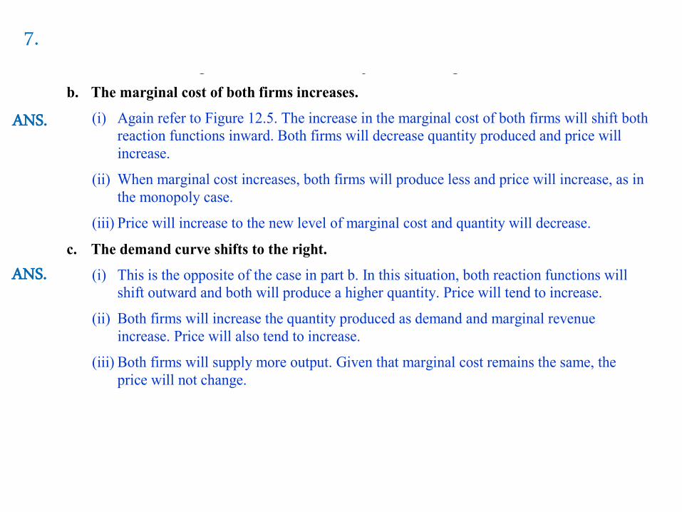
b. The marginal cost of both firms increases.

(i) Again refer to Figure 12.5. The increase in the marginal cost of both firms will shift both

reaction functions inward. Both firms will decrease quantity produced and price will

increase.

(ii) When marginal cost increases, both firms will produce less and price will increase, as in

the monopoly case.

(iii) Price will increase to the new level of marginal cost and quantity will decrease.

c. The demand curve shifts to the right.

(i) This is the opposite of the case in part b. In this situation, both reaction functions will

shift outward and both will produce a higher quantity. Price will tend to increase.

(ii) Both firms will increase the quantity produced as demand and marginal revenue

increase. Price will also tend to increase.

(iii) Both firms will supply more output. Given that marginal cost remains the same, the

price will not change.

ANS.

7. Suppose that two competing firms, A and B, produce a homogeneous good. Both firms have

a marginal cost of MC $50. Describe what would happen to output and price in each of

the following situations if the firms are at (i) Cournot equilibrium, (ii) collusive

equilibrium, and (iii) Bertrand equilibrium.

a. Because Firm A must increase wages, its MC increases to $80.

(i) In a Cournot equilibrium you must think about the effect on the reaction functions, as

illustrated in Figure 12.5 of the text. When Firm A experiences an increase in marginal

cost, its reaction function will shift inward. The quantity produced by Firm A will

decrease and the quantity produced by Firm B will increase. Total quantity produced

will decrease and price will increase.

(ii) In a collusive equilibrium, the two firms will collectively act like a monopolist. When

the marginal cost of Firm A increases, Firm A will reduce its production to zero, because

Firm B can produce at a lower marginal cost. Because Firm B can produce the entire

industry output at a marginal cost of $50, there will be no change in output or price.

However, the firms will have to come to some agreement on how to share the profit

earned by B.

(iii) Before the increase in Firm A’s costs, both firms would charge a price equal to marginal

cost (P $50) because the good is homogeneous. After Firm A’s marginal cost

increases, Firm B will raise its price to $79.99 (or some price just below $80) and take

all sales away from Firm A. Firm A would lose money on each unit sold at any price

below its marginal cost of $80, so it will produce nothing.

b. The marginal cost of both firms increases.

(i) Again refer to Figure 12.5. The increase in the marginal cost of both firms will shift both

reaction functions inward. Both firms will decrease quantity produced and price will

increase.

(ii) When marginal cost increases, both firms will produce less and price will increase, as in

the monopoly case.

(iii) Price will increase to the new level of marginal cost and quantity will decrease.

c. The demand curve shifts to the right.

(i) This is the opposite of the case in part b. In this situation, both reaction functions will

shift outward and both will produce a higher quantity. Price will tend to increase.

(ii) Both firms will increase the quantity produced as demand and marginal revenue

increase. Price will also tend to increase.

(iii) Both firms will supply more output. Given that marginal cost remains the same, the

price will not change.

7.

ANS.

ANS.

Competition versus Collusion:

The Prisoners’ Dilemma12.4

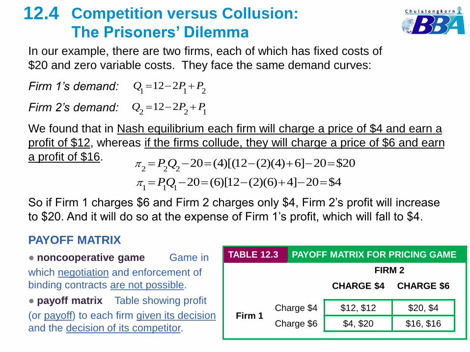
In our example, there are two firms, each of which has fixed costs of

$20 and zero variable costs. They face the same demand curves:

Firm 1’s demand:

Firm 2’s demand:

We found that in Nash equilibrium each firm will charge a price of $4 and earn a

profit of $12, whereas if the firms collude, they will charge a price of $6 and earn

a profit of $16.

So if Firm 1 charges $6 and Firm 2 charges only $4, Firm 2’s profit will increase

to $20. And it will do so at the expense of Firm 1’s profit, which will fall to $4.

1 1 212 2Q P P

2 2 112 2Q P P

2 2 220 (4)[(12 (2)(4) 6] 20 $20P Q

1 1 120 (6)[12 (2)(6) 4] 20 $4PQ

TABLE 12.3 PAYOFF MATRIX FOR PRICING GAME

FIRM 2

CHARGE $4 CHARGE $6

Firm 1Charge $4 $12, $12 $20, $4

Charge $6 $4, $20 $16, $16

● payoff matrix Table showing profit

(or payoff) to each firm given its decision

and the decision of its competitor.

● noncooperative game Game in

which negotiation and enforcement of

binding contracts are not possible.

PAYOFF MATRIX

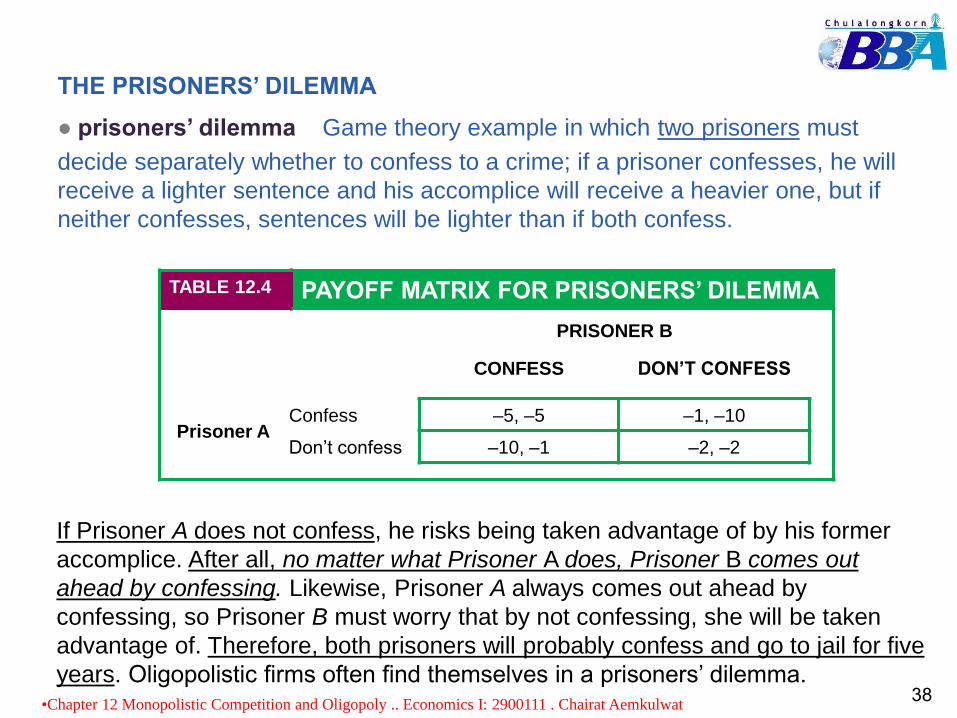
THE PRISONERS’ DILEMMA

TABLE 12.4 PAYOFF MATRIX FOR PRISONERS’ DILEMMA

PRISONER B

CONFESS DON’T CONFESS

Prisoner AConfess –5, –5 –1, –10

Don’t confess –10, –1 –2, –2

● prisoners’ dilemma Game theory example in which two prisoners must

decide separately whether to confess to a crime; if a prisoner confesses, he will

receive a lighter sentence and his accomplice will receive a heavier one, but if

neither confesses, sentences will be lighter than if both confess.

If Prisoner A does not confess, he risks being taken advantage of by his former

accomplice. After all, no matter what Prisoner A does, Prisoner B comes out

ahead by confessing. Likewise, Prisoner A always comes out ahead by

confessing, so Prisoner B must worry that by not confessing, she will be taken

advantage of. Therefore, both prisoners will probably confess and go to jail for five

years. Oligopolistic firms often find themselves in a prisoners’ dilemma.•Chapter 12 Monopolistic Competition and Oligopoly .. Economics I: 2900111 . Chairat Aemkulwat

38

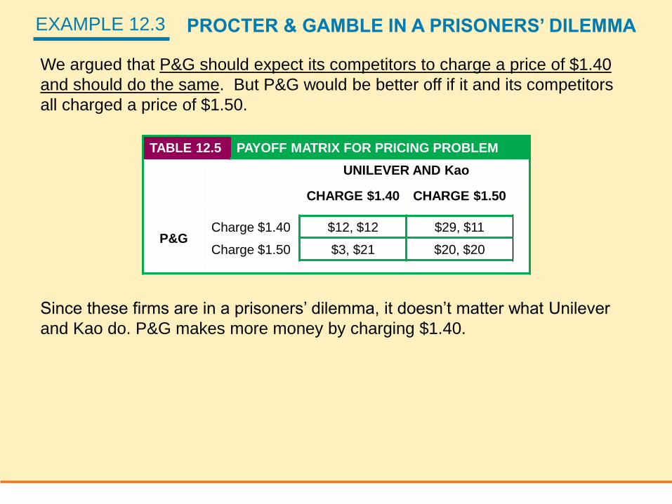
EXAMPLE 12.3 PROCTER & GAMBLE IN A PRISONERS’ DILEMMA

We argued that P&G should expect its competitors to charge a price of $1.40

and should do the same. But P&G would be better off if it and its competitors

all charged a price of $1.50.

TABLE 12.5 PAYOFF MATRIX FOR PRICING PROBLEM

UNILEVER AND Kao

CHARGE $1.40 CHARGE $1.50

P&GCharge $1.40 $12, $12 $29, $11

Charge $1.50 $3, $21 $20, $20

Since these firms are in a prisoners’ dilemma, it doesn’t matter what Unilever

and Kao do. P&G makes more money by charging $1.40.

Implications of the Prisoners’

Dilemma for Oligopolistic Pricing

12.5

Price Rigidity

● price rigidity Characteristic of oligopolistic markets by which firms are

reluctant to change prices even if costs or demands change.

● kinked demand curve model Oligopoly model in which each firm faces a

demand curve kinked at the currently prevailing price: at higher prices demand

is very elastic, whereas at lower prices it is inelastic.

Does the prisoners’ dilemma doom oligopolistic firms to aggressive competition

and low profits? Not necessarily. Although our imaginary prisoners have only

one opportunity to confess, most firms set output and price over and over

again, continually observing their competitors’ behavior and adjusting their own

accordingly. This allows firms to develop reputations from which trust can arise.

As a result, oligopolistic coordination and cooperation can sometimes prevail.


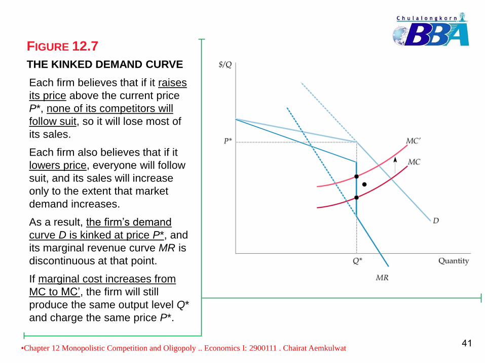
THE KINKED DEMAND CURVE

FIGURE 12.7

Each firm believes that if it raises

its price above the current price

P*, none of its competitors will

follow suit, so it will lose most of

its sales.

Each firm also believes that if it

lowers price, everyone will follow

suit, and its sales will increase

only to the extent that market

demand increases.

As a result, the firm’s demand

curve D is kinked at price P*, and

its marginal revenue curve MR is

discontinuous at that point.

If marginal cost increases from

MC to MC’, the firm will still

produce the same output level Q*

and charge the same price P*.


Price Signaling and Price Leadership

● price signaling Form of implicit collusion in which a firm announces a price

increase in the hope that other firms will follow suit.

● price leadership Pattern of pricing in which one firm regularly announces

price changes that other firms then match.

In some industries, a large firm might naturally emerge as a leader, with the

other firms deciding that they are best off just matching the leader’s prices,

rather than trying to undercut the leader or each other.

Price leadership can also serve as a way for oligopolistic firms to deal with the

reluctance to change prices, a reluctance that arises out of the fear of being

undercut or “rocking the boat.”


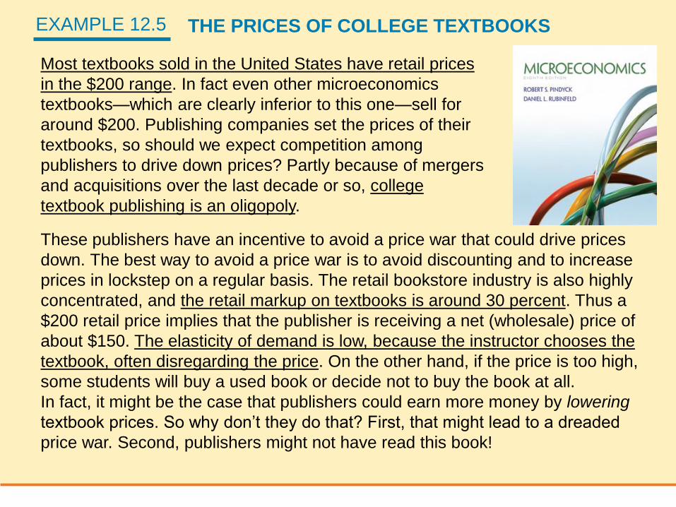
EXAMPLE 12.5 THE PRICES OF COLLEGE TEXTBOOKS

Most textbooks sold in the United States have retail prices

in the $200 range. In fact even other microeconomics

textbooks—which are clearly inferior to this one—sell for

around $200. Publishing companies set the prices of their

textbooks, so should we expect competition among

publishers to drive down prices? Partly because of mergers

and acquisitions over the last decade or so, college

textbook publishing is an oligopoly.

These publishers have an incentive to avoid a price war that could drive prices

down. The best way to avoid a price war is to avoid discounting and to increase

prices in lockstep on a regular basis. The retail bookstore industry is also highly

concentrated, and the retail markup on textbooks is around 30 percent. Thus a

$200 retail price implies that the publisher is receiving a net (wholesale) price of

about $150. The elasticity of demand is low, because the instructor chooses the

textbook, often disregarding the price. On the other hand, if the price is too high,

some students will buy a used book or decide not to buy the book at all.

In fact, it might be the case that publishers could earn more money by lowering

textbook prices. So why don’t they do that? First, that might lead to a dreaded

price war. Second, publishers might not have read this book!

IMPLICATIONS OF THE PRISONERS’ DILEMMA

FOR OLIGOPOLISTIC PRICING12.5

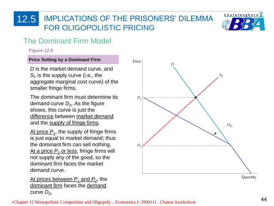
The Dominant Firm Model

D is the market demand curve, and

SF is the supply curve (i.e., the

aggregate marginal cost curve) of the

smaller fringe firms.

The dominant firm must determine its

demand curve DD. As the figure

shows, this curve is just the

difference between market demand

and the supply of fringe firms.

At price P1, the supply of fringe firms

is just equal to market demand; thus

the dominant firm can sell nothing.

At a price P2 or less, fringe firms will

not supply any of the good, so the

dominant firm faces the market

demand curve.

At prices between P1 and P2, the

dominant firm faces the demand

curve DD.

Price Setting by a Dominant Firm

Figure 12.9


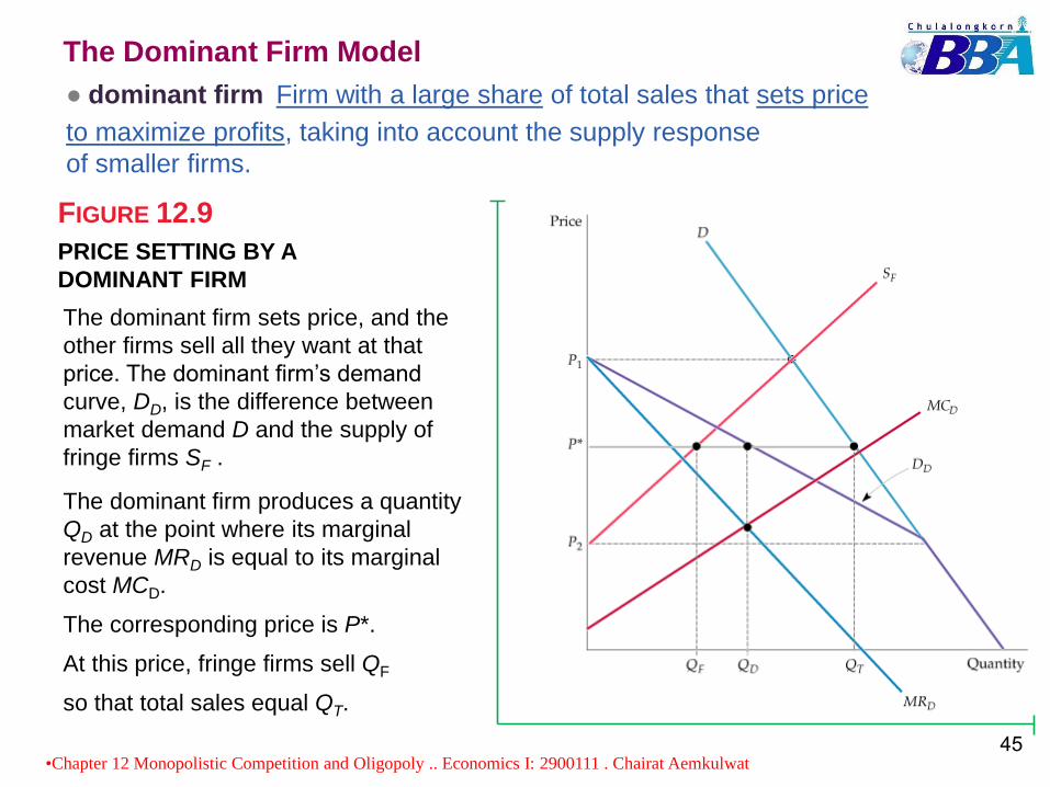
PRICE SETTING BY A

DOMINANT FIRM

FIGURE 12.9

The Dominant Firm Model

● dominant firm Firm with a large share of total sales that sets price

to maximize profits, taking into account the supply response

of smaller firms.

The dominant firm sets price, and the

other firms sell all they want at that

price. The dominant firm’s demand

curve, DD, is the difference between

market demand D and the supply of

fringe firms SF .

The dominant firm produces a quantity

QD at the point where its marginal

revenue MRD is equal to its marginal

cost MCD.

The corresponding price is P*.

At this price, fringe firms sell QF

so that total sales equal QT.


Cartels12.6

Producers in a cartel explicitly agree to cooperate in setting

prices and output levels. • If enough producers adhere to the cartel’s agreements, and if market

demand is sufficiently inelastic, the cartel may drive prices well above

competitive levels.

Cartels are often international. • While U.S. antitrust laws prohibit American companies from colluding, those

of other countries are much weaker and are sometimes poorly enforced.

• Furthermore, nothing prevents countries, or companies owned or controlled

by foreign governments, from forming cartels.

• For example, the OPEC cartel is an international agreement among oil-

producing countries which has succeeded in raising world oil prices above

competitive levels.


First, a stable cartel organization must be formed whose members agree on

price and production levels and then adhere to that agreement.

The second condition, and may be the most important, is the potential for

monopoly power. Even if a cartel can solve its organizational problems, there

will be little room to raise price if it faces a highly elastic demand curve.

CONDITIONS FOR CARTEL SUCCESS

Analysis of Cartel Pricing

Cartel pricing can be analyzed by using the dominant firm model discussed

earlier. We will apply this model to two cartels, the OPEC oil cartel and the

CIPEC copper cartel. This will help us understand why OPEC was successful

in raising price while CIPEC was not.


ANALYZING OPEC

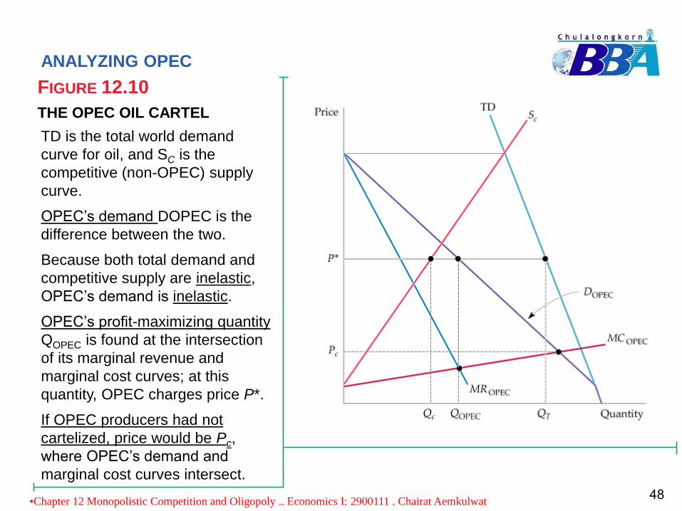
THE OPEC OIL CARTEL

FIGURE 12.10

TD is the total world demand

curve for oil, and SC is the

competitive (non-OPEC) supply

curve.

OPEC’s demand DOPEC is the

difference between the two.

Because both total demand and

competitive supply are inelastic,

OPEC’s demand is inelastic.

OPEC’s profit-maximizing quantity

QOPEC is found at the intersection

of its marginal revenue and

marginal cost curves; at this

quantity, OPEC charges price P*.

If OPEC producers had not

cartelized, price would be Pc,

where OPEC’s demand and

marginal cost curves intersect.


ANALYZING CIPEC

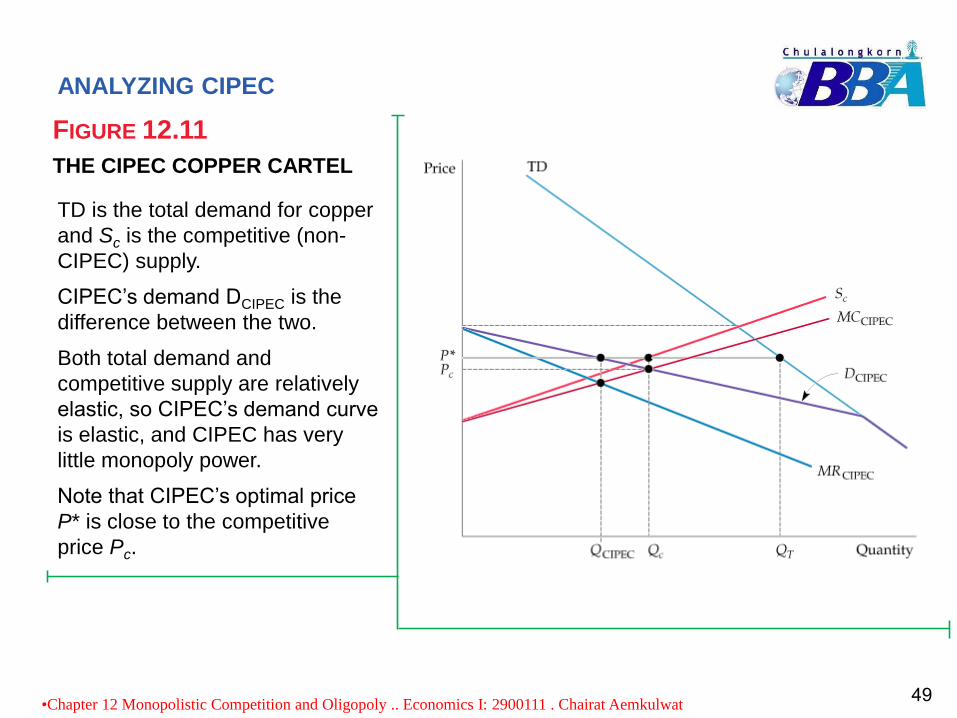
THE CIPEC COPPER CARTEL

FIGURE 12.11

TD is the total demand for copper

and Sc is the competitive (non-

CIPEC) supply.

CIPEC’s demand DCIPEC is the

difference between the two.

Both total demand and

competitive supply are relatively

elastic, so CIPEC’s demand curve

is elastic, and CIPEC has very

little monopoly power.

Note that CIPEC’s optimal price

P* is close to the competitive

price Pc.


As the examples of OPEC and CIPEC illustrate, successful cartelization

requires two things:

First, the total demand for the good must not be very price elastic.

Second, either the cartel must control nearly all the world’s supply or, if it does

not, the supply of noncartel producers must not be price elastic.

Most international commodity cartels have failed because few world markets

meet both conditions.


EXAMPLE 12.7 THE MILK CARTEL

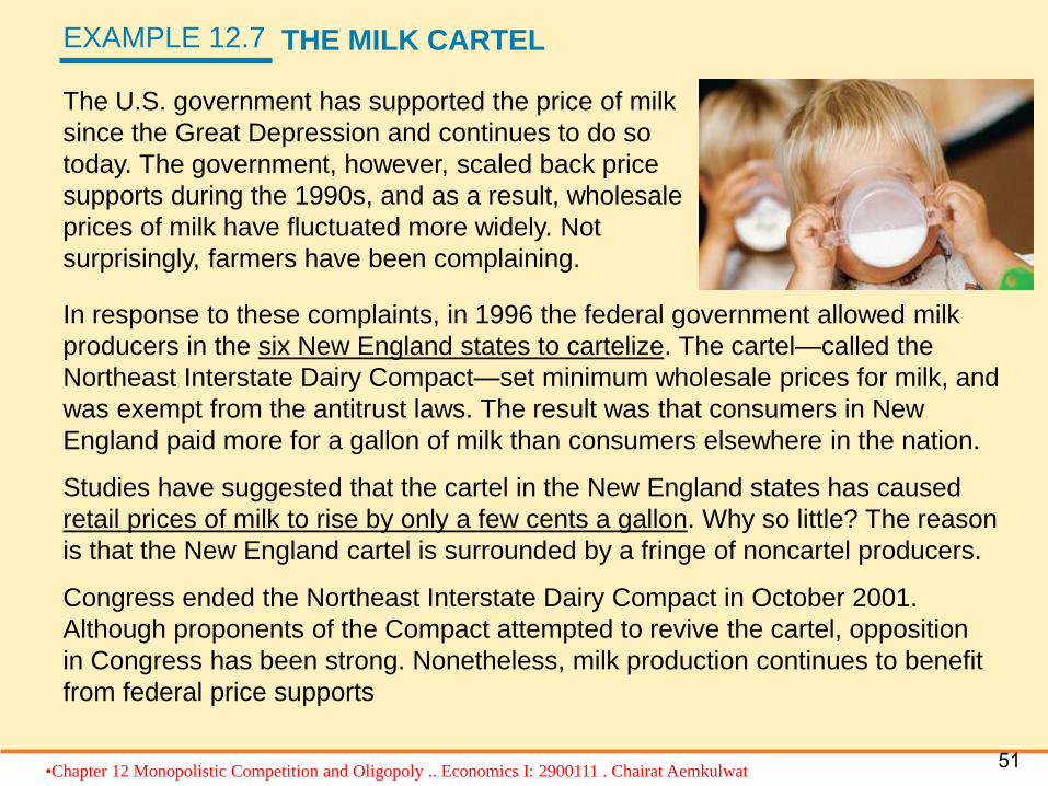
The U.S. government has supported the price of milk

since the Great Depression and continues to do so

today. The government, however, scaled back price

supports during the 1990s, and as a result, wholesale

prices of milk have fluctuated more widely. Not

surprisingly, farmers have been complaining.

In response to these complaints, in 1996 the federal government allowed milk

producers in the six New England states to cartelize. The cartel—called the

Northeast Interstate Dairy Compact—set minimum wholesale prices for milk, and

was exempt from the antitrust laws. The result was that consumers in New

England paid more for a gallon of milk than consumers elsewhere in the nation.

Studies have suggested that the cartel in the New England states has caused

retail prices of milk to rise by only a few cents a gallon. Why so little? The reason

is that the New England cartel is surrounded by a fringe of noncartel producers.

Congress ended the Northeast Interstate Dairy Compact in October 2001.

Although proponents of the Compact attempted to revive the cartel, opposition

in Congress has been strong. Nonetheless, milk production continues to benefit

from federal price supports


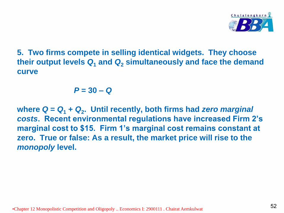
5. Two firms compete in selling identical widgets. They choose

their output levels Q1 and Q2 simultaneously and face the demand

curve

P = 30 – Q

where Q = Q1 + Q2. Until recently, both firms had zero marginal

costs. Recent environmental regulations have increased Firm 2’s

marginal cost to $15. Firm 1’s marginal cost remains constant at

zero. True or false: As a result, the market price will rise to the

monopoly level.


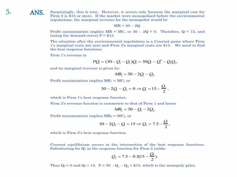
Surprisingly, this is true. However, it occurs only because the marginal cost for

Firm 2 is $15 or more. If the market were monopolized before the environmental

regulations, the marginal revenue for the monopolist would be

MR = 30 – 2Q.

Profit maximization implies MR = MC, or 30 – 2Q = 0. Therefore, Q = 15, and

(using the demand curve) P = $15.

The situation after the environmental regulations is a Cournot game where Firm

1's marginal costs are zero and Firm 2's marginal costs are $15. We need to find

the best response functions:

Firm 1’s revenue is

PQ1 (30Q1 Q2 )Q1 30Q1 Q1

2Q1Q2,

and its marginal revenue is given by:

MR1 30 2Q1 Q2.

Profit maximization implies MR1 = MC1 or

30 2Q1 Q2 0 Q1 15Q2

2,

which is Firm 1’s best response function.

Firm 2’s revenue function is symmetric to that of Firm 1 and hence

MR2 30 Q1 2Q2.

Profit maximization implies MR2 = MC2, or

30 2Q2 Q1 15 Q2 7.5Q1

2,

which is Firm 2’s best response function.

Cournot equilibrium occurs at the intersection of the best response functions.

Substituting for Q1 in the response function for Firm 2 yields:

Q2 7.5 0.5(15 Q2

2).

Thus Q2 = 0 and Q1 = 15. P = 30 – Q1 – Q2 = $15, which is the monopoly price.

ANS.5.

Recap: Chapter 12

• Monopolistic Competition

• Oligopoly

• Price Competition

• Competition versus Collusion:

• The Prisoners’ Dilemma

• Implications of the Prisoners’ Dilemma for

Oligopolistic Pricing

• Cartels

•Chapter 12 Monopolistic Competition and Oligopoly .. Economics I: 2900111 . Chairat Aemkulwat

Documents

12 Monopolistic Competition and Oligopolypioneer.netserv.chula.ac.th/~achairat/12_Monopolistic... · · 2017-04-1812.2 Oligopoly 12.3 Price Competition ... 11. 1. Suppose all firms