A Guide to Using OLI Analyzer 210

12. Petroleum Calculations

Overview Calculations with the OLI Software can be used to characterize crude oils. Here is a quote from the OLI Tricks of the Trade manual (AQSim)

Crude oils are complex groups of organic molecules containing hundreds, perhaps thousands of pure components in a single oil. Modeling crude oils using pure components is impractical, because analyzing for each pure component is cost prohibitive and the number of species would make calculations overwhelming. A convenient solution to this problem and to modeling the properties of a crude oil is to create pseudo components. Crude Oil properties may be defined through a distillation curve, where each boiling point range is a progression of molecular weights, densities, solubilities, viscosities and other properties associated with that section. It is reasonable for low boiling point molecules to be low molecular weight, low density, low viscosity, and more soluble in water. We can dice boiling point curves using well accepted methods standard to create pseudocomponents that in combination reflect the property of the whole oil.

There are two ways to create a crude oil stream on the Analyzers. The first is to start with a PVT curve and create pseudocomponents using one of the three thermodynamic methods coded into the software. The second is to enter the pseudocomponent data directly and using the same thermodynamic methods to predict the component properties.

The three thermodynamic methods are API, Lee Kesler, and Cavett. At the time of writing, the software implementation specifications for these methods were not in hand.

This involves taking distillation data (such as ASTM D86) and converting that information into properties that the OLI software can use. This is generally referred to as “Creating Pseudo Components.”

There are two classes of this type of data. Actual assay (or distillation data) in which we cut the boiling point curves up into individual components or the actual entering of a pseudocomponent.

This section shows you how to enter each method.

Assays For this example we will enter a distillation curve for a sample crude oil. This sample used ASTM method D86 to characterize the crude oil (see Chapter 13 on page 224 for a description of the distillation methods). The data for the distillation curve can be found in Table 12-1 on page 211.

A Guide to Using OLI Analyzer 211

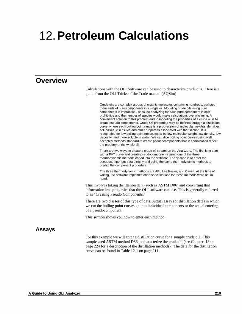
Table 12-1 Sample Distillation data using ASTM method D86, API Gravity of 31

Distillation Data

Volume Percent Distilled Temperature, C

1 20

5 30

10 50

20 60

40 80

60 120

80 150

90 180

95 200

99 220

100 240

Create a standard OLI Studio stream at the following conditions

Stream Name Crude

Temperature 25 oC

Pressure 1.0 atmospheres

H2O 5 moles

You will need to enter the name of the assay. In our example we are using the name “Assay”. You are limited to only 5 characters for the name of the assay.

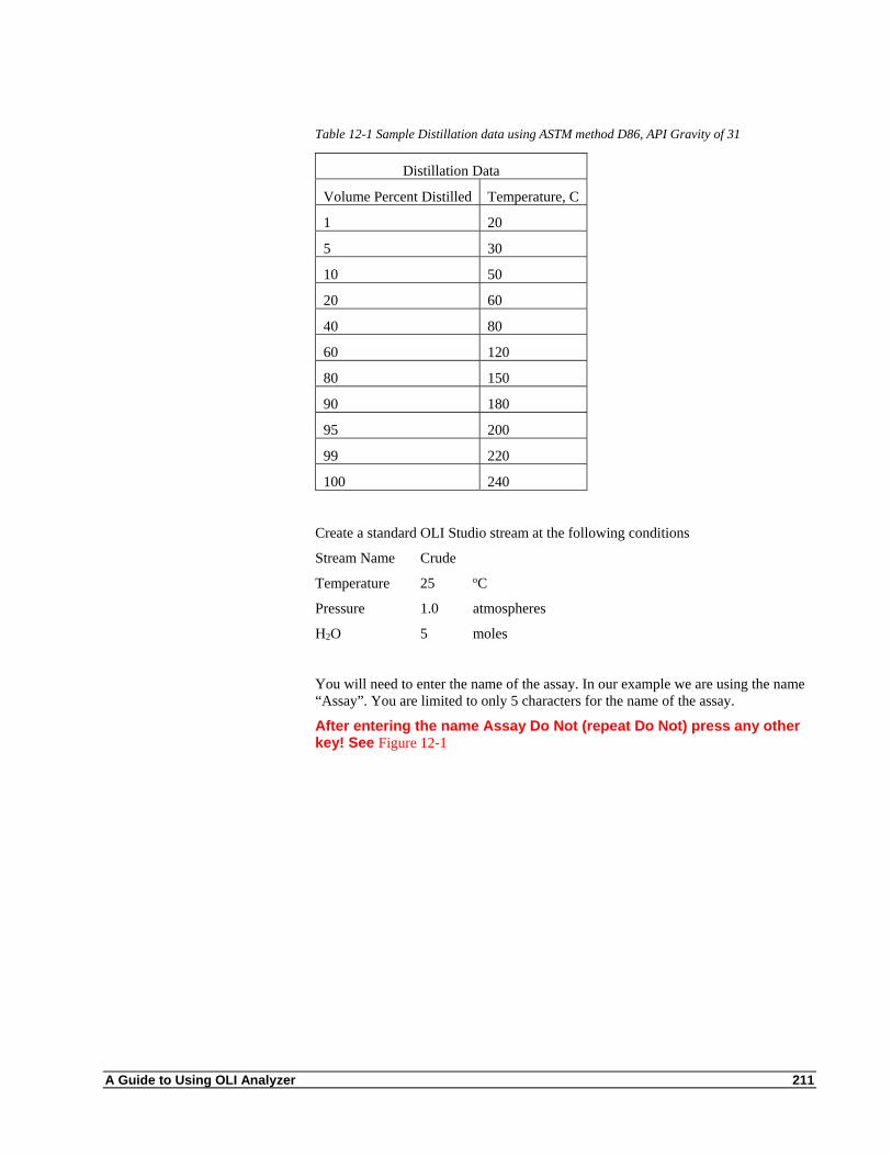
After entering the name Assay Do Not (repeat Do Not) press any other key! See Figure 12-1

A Guide to Using OLI Analyzer 212

Figure 12-1 Entering a petroleum sample, Don't press ENTER yet!

The OLI Analyzer requires a different series of key strokes to enable the entering of the assay data.

After typing the name “Assay” you will need to use the following key combination

Shift – Enter

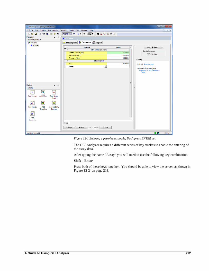
Press both of these keys together. You should be able to view the screen as shown in Figure 12-2 on page 213.

A Guide to Using OLI Analyzer 213

Figure 12-2 Blank Assay input grids

We will begin by defining the type of assay data. Click in the cell next to the

Assay Data Type to see a list of distillation types.

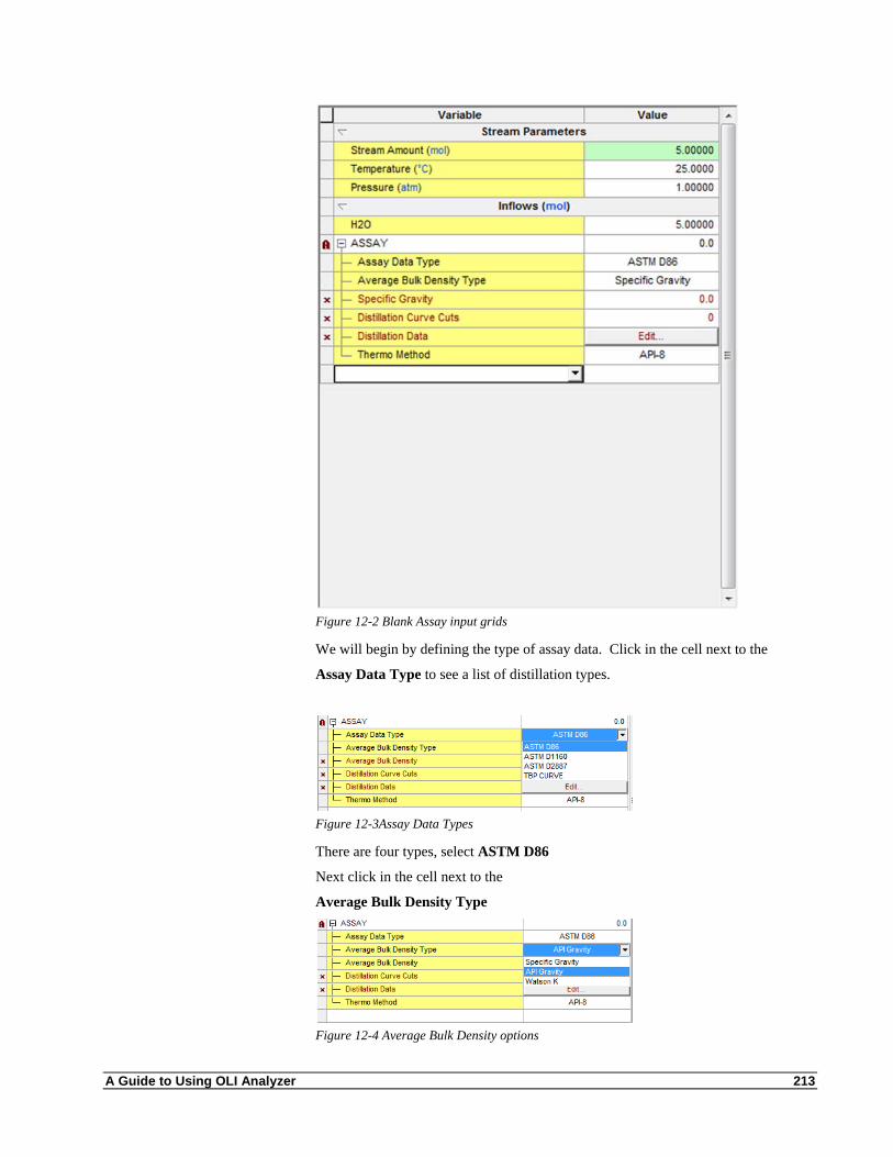
Figure 12-3Assay Data Types

There are four types, select ASTM D86

Next click in the cell next to the

Average Bulk Density Type

Figure 12-4 Average Bulk Density options

A Guide to Using OLI Analyzer 214

There are three types (see 13 on page 224)

Select API Gravity

Finally we need to select the thermodynamic method. Click in the cell next to

Thermo Method

There are four types (see 13 on page 224)

Figure 12-5 Thermodynamic methods

Select API-8 (Default)

We are now ready to enter the distillation data. Click the Edit button next to the

Distillation Data cell. You should see Figure 12-6 below

Figure 12-6 Blank Distillation Data, cut and paste works here!

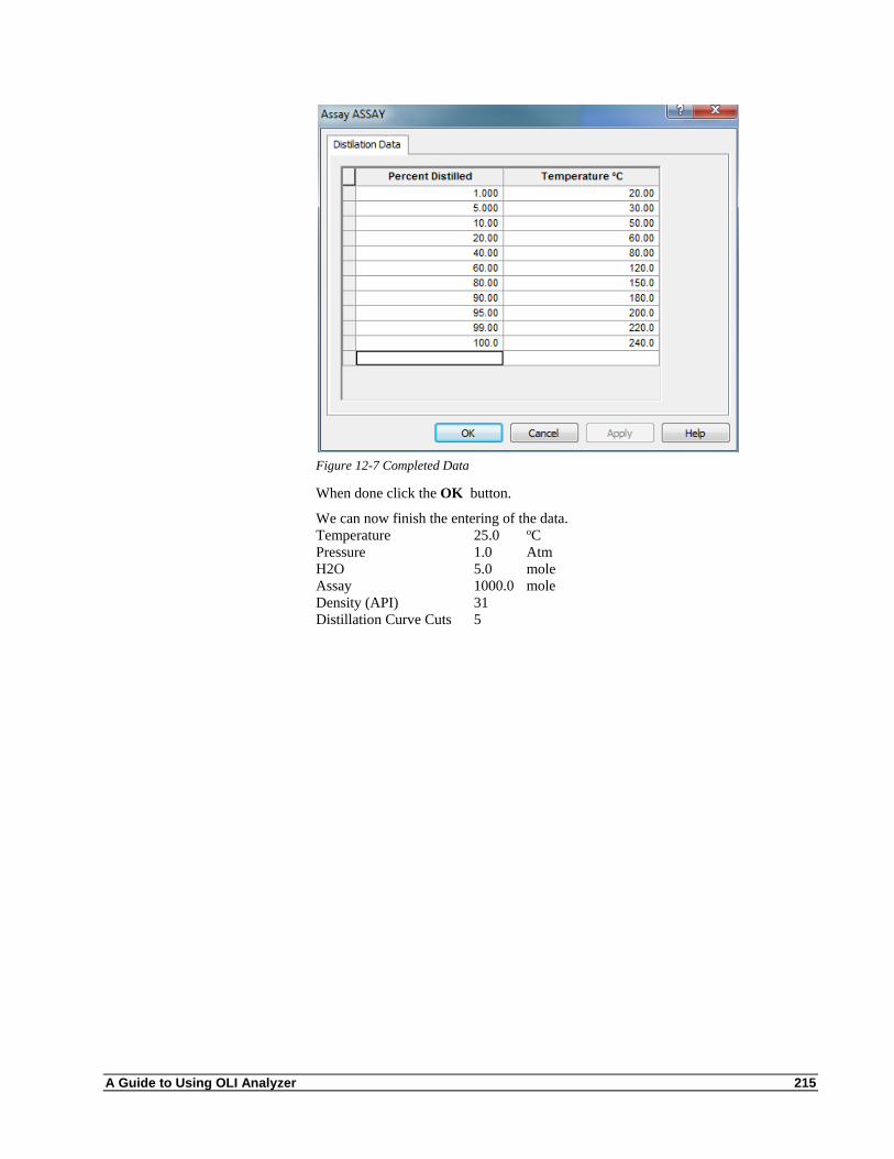
Enter the data from Table 12-1on page 211

A Guide to Using OLI Analyzer 215

Figure 12-7 Completed Data

When done click the OK button.

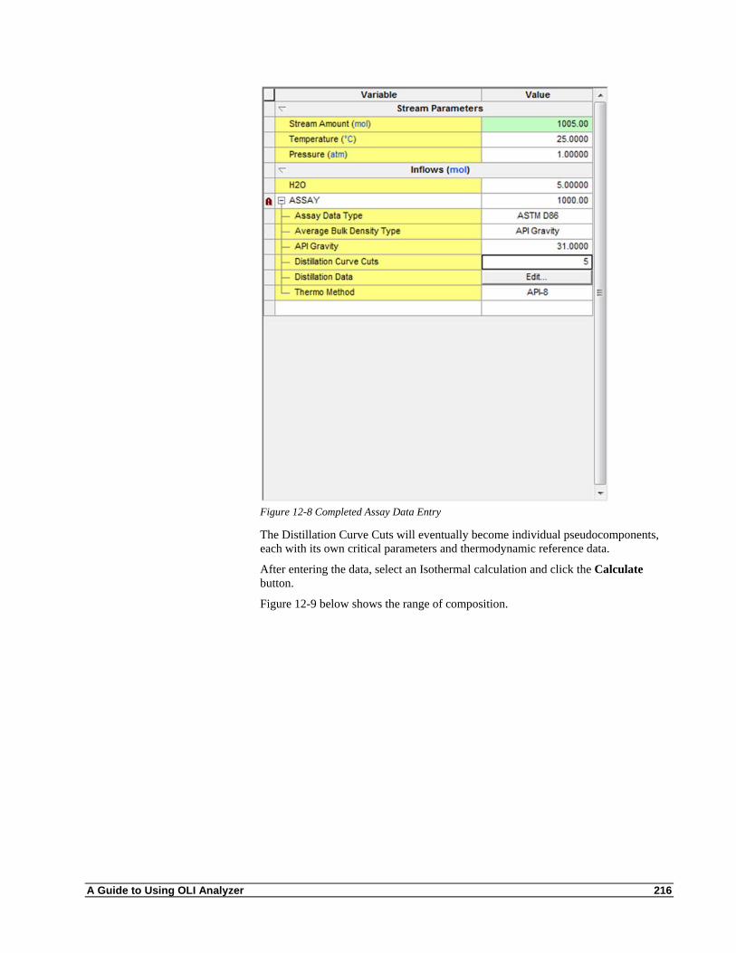
We can now finish the entering of the data. Temperature 25.0 oC Pressure 1.0 Atm H2O 5.0 mole Assay 1000.0 mole Density (API) 31 Distillation Curve Cuts 5

A Guide to Using OLI Analyzer 216

Figure 12-8 Completed Assay Data Entry

The Distillation Curve Cuts will eventually become individual pseudocomponents, each with its own critical parameters and thermodynamic reference data.

After entering the data, select an Isothermal calculation and click the Calculate button.

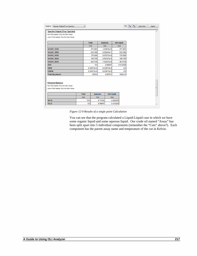
Figure 12-9 below shows the range of composition.

A Guide to Using OLI Analyzer 217

Figure 12-9 Results of a single point Calculation

You can see that the program calculated a Liquid-Liquid case in which we have some organic liquid and some aqueous liquid. Our crude oil named “Assay” has been split apart into 5 individual components (remember the “Cuts” above?). Each component has the parent assay name and temperature of the cut in Kelvin.

A Guide to Using OLI Analyzer 218

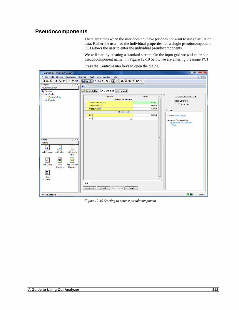
Pseudocomponents There are times when the user does not have (or does not want to use) distillation data. Rather the user had the individual properties for a single pseudocomponent. OLI allows the user to enter the individual pseudocomponents.

We will start by creating a standard stream. On the input grid we will enter our pseudocomponent name. In Figure 12-10 below we are entering the name PC1.

Press the Control-Enter keys to open the dialog.

Figure 12-10 Starting to enter a pseudocomponent

A Guide to Using OLI Analyzer 219

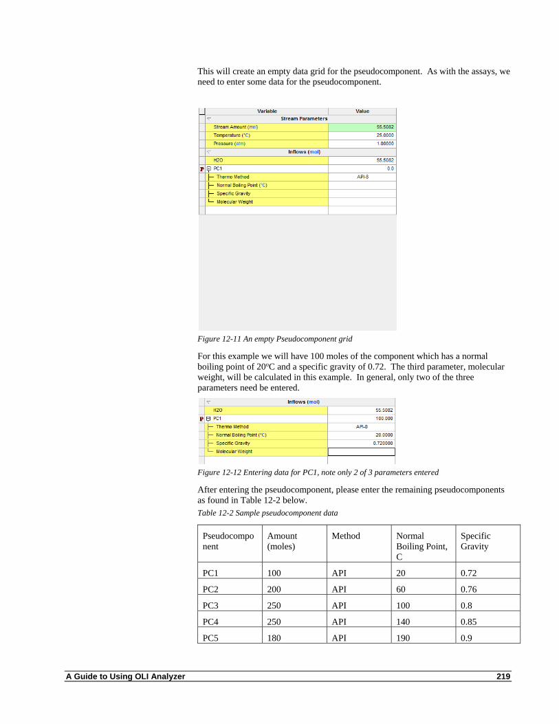
This will create an empty data grid for the pseudocomponent. As with the assays, we need to enter some data for the pseudocomponent.

Figure 12-11 An empty Pseudocomponent grid

For this example we will have 100 moles of the component which has a normal boiling point of 20oC and a specific gravity of 0.72. The third parameter, molecular weight, will be calculated in this example. In general, only two of the three parameters need be entered.

Figure 12-12 Entering data for PC1, note only 2 of 3 parameters entered

After entering the pseudocomponent, please enter the remaining pseudocomponents as found in Table 12-2 below. Table 12-2 Sample pseudocomponent data

Pseudocomponent

Amount (moles)

Method Normal Boiling Point, C

Specific Gravity

PC1 100 API 20 0.72

PC2 200 API 60 0.76

PC3 250 API 100 0.8

PC4 250 API 140 0.85

PC5 180 API 190 0.9

A Guide to Using OLI Analyzer 220

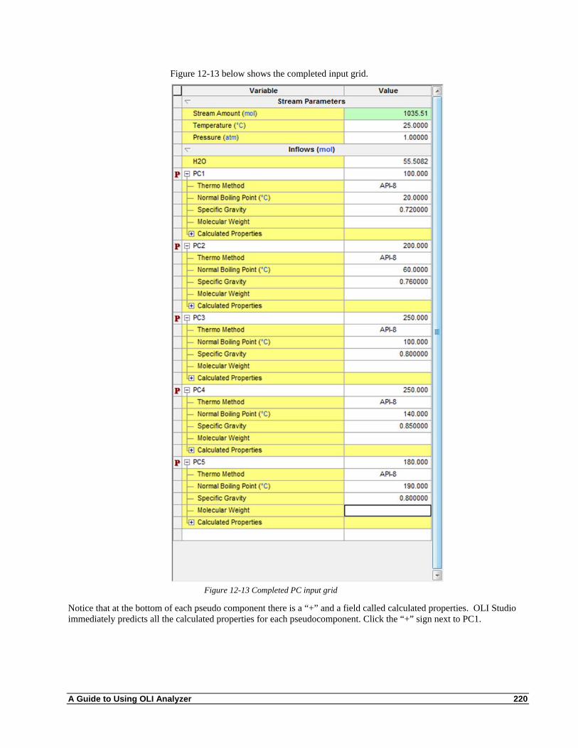
Figure 12-13 below shows the completed input grid.

Figure 12-13 Completed PC input grid

Notice that at the bottom of each pseudo component there is a “+” and a field called calculated properties. OLI Studio immediately predicts all the calculated properties for each pseudocomponent. Click the “+” sign next to PC1.

A Guide to Using OLI Analyzer 221

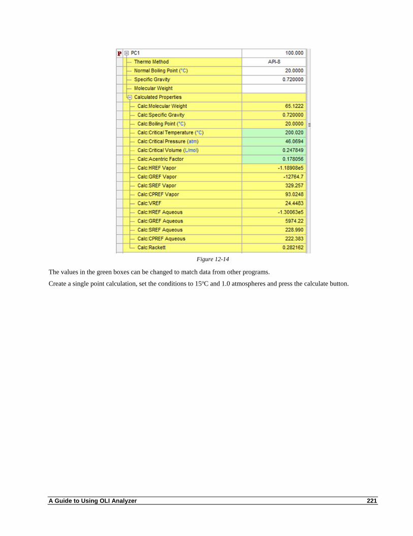
Figure 12-14

The values in the green boxes can be changed to match data from other programs.

Create a single point calculation, set the conditions to 15oC and 1.0 atmospheres and press the calculate button.

A Guide to Using OLI Analyzer 222

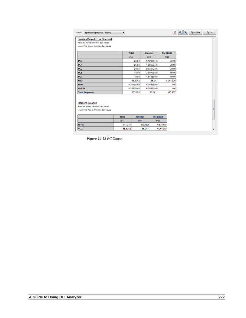
Figure 12-15 PC Output

A Guide to Using OLI Analyzer 223