1.2 Second-order systems - MIT OpenCourseWare · PDF fileIn the basic linear models considered here, ... SECOND-ORDER SYSTEMS 29 • First, ... exponentials are the natural response

1.2. SECOND-ORDER SYSTEMS 25

if the initial fluid height is defined as h(0) = h0, then the fluid height as a function of time varies as

h(t) = h0e!t!g/RA [m]. (1.31)

1.2 Second-order systems

In the previous sections, all the systems had only one energy storage element, and thus could be modeled by a first-order di!erential equation. In the case of the mechanical systems, energy was stored in a spring or an inertia. In the case of electrical systems, energy can be stored either in a capacitance or an inductance. In the basic linear models considered here, thermal systems store energy in thermal capacitance, but there is no thermal equivalent of a second means of storing energy. That is, there is no equivalent of a thermal inertia. Fluid systems store energy via pressure in fluid capacitances, and via flow rate in fluid inertia (inductance).

In the following sections, we address models with two energy storage elements. The simple step of adding an additional energy storage element allows much greater variation in the types of responses we will encounter. The largest di!erence is that systems can now exhibit oscillations in time in their natural response. These types of responses are su"ciently important that we will take time to characterize them in detail. We will first consider a second-order mechanical system in some depth, and use this to introduce key ideas associated with second-order responses. We then consider second-order electrical, thermal, and fluid systems.

1.2.1 Complex numbers

In our consideration of second-order systems, the natural frequencies are in general complex-valued. We only need a limited set of complex mathematics, but you will need to have good facility with complex number manipulations and identities. For a review of complex numbers, take a look at the handout on the course web page.

1.2.2 Mechanical second-order system

The second-order system which we will study in this section is shown in Figure 1.19. As shown in the figure, the system consists of a spring and damper attached to a mass which moves laterally on a frictionless surface. The lateral position of the mass is denoted as x. As before, the zero of

26 CHAPTER 1. NATURAL RESPONSE

m

k

b

x

Frictionless�support

Figure 1.19: Second-order mechanical system.

position is indicated in the figure by the vertical line connecting to the arrow which indicates the direction of increasing x.

A free-body diagram for the system is shown in Figure 1.20. The forces Fk and Fb are identical to those considered in Section 1.1.1. That is, the spring is extended by a force proportional to motion in the x-direction, Fk = kx. The damper is translated by a force which is proportional to velocity in the x-direction, Fb = b dx/dt. As shown in the free-body diagram, these forces have a reaction component acting in the opposite direction on the mass m. The only di!erence here as compared to the first-order system of Section 1.1.1 is that here the moving element has finite mass m. In Section 1.1.1 the link was massless.

To write the system equation of motion, you sum the forces acting on the mass, taking care to keep track of the reference direction associated with these forces. Through Newton’s second law the sum of these forces is equal to the mass times acceleration

dx d 2x !Fb ! Fk = !b dt ! kx = m . (1.32)

dt2

Rearranging yields the system equation in standard form

d 2x dx m + b + kx = 0. (1.33)

dt2 dt

(As a check on your understanding, convince yourself that the units of all the terms in this equation are force [N].)

27 1.2. SECOND-ORDER SYSTEMS

x

k Fk

Fb b

x

System�cut�here Forces�acting�on�elements

Frictionless�support

m

Figure 1.20: Free body diagram for second-order system.

Initial condition response

For this second-order system, initial conditions on both the position and velocity are required to specify the state. The response of this system to an initial displacement x(0) = x0 and initial velocity v(0) = x(0) = v0

is found in a manner identical to that previously used in the first order case of Section 1.1. That is, assume that x(t) takes the form x(t) = cest . Substituting this function into (1.33) and applying the derivative property of the exponential yields

ms 2 ce st + bscest + kcest = 0. (1.34)

As before, the common factor cest may be cancelled, since it is nonzero for any finite s and t, and with non-rest (c = 0) initial conditions. Thus we "find that s must satisfy the characteristic equation ms2 + bs + k = 0. This second-order polynomial has two solutions

b #

b2 ! 4mk s1 = !

2m +

2m (1.35)

and b

#b2 ! 4mk

s2 = !2m

! 2m

(1.36)

which are the pole locations (natural frequencies) of the system.


In most cases, the poles are distinct (b2 = 4" mk), and the initial condition response will take the form

x(t) = c1e s1t + c2e s2t (1.37)

where s1 and s2 are given above, and the two constants c1 and c2 are chosen to satisfy the initial conditions x0 and v0. If the roots are real (b2 > 4mk), then the response is the weighted sum of two real exponentials. If the roots have an imaginary component (b2 < 4mk), then the exponentials are complex and the response has an oscillatory component. Since in this case s1 = s2

", in order to have a real response it must hold that c1 = c2", and

thus the response can be expressed as x(t) = 2Re{c1es1t}, or equivalently as x(t) = 2Re{c2es2t}.

In the case that the poles are coincident (b2 = 4mk), we have s1 = s2, and the initial condition response will take the form

x(t) = c1e s1t + c2tes1t (1.38)

As before, the two constants c1 and c2 are chosen to satisfy the initial conditions x0 and v0.

Before further analysis, it is helpful to introduce some standard terms. The pole locations are conveniently parameterized in terms of the damping ratio !, and natural frequency "n, where

! k

(1.40)

"n = m

(1.39)

and b

! = . 2#

km

The natural frequency "n is the frequency at which the system would oscillate if the damping b were zero. The damping ratio ! is the ratio of the actual damping b to the critical damping bc = 2

#km. You should see that

the critical damping value is the value for which the poles are coincident. In terms of these parameters, the di!erential equation (1.33) takes the

form 1 d 2x 2! dx

+ + x = 0. (1.41)"2 dt2 "n dtn

In the following section we will make the physically reasonable assumption that the values of m, and k are greater than zero (to maintain system order) and that b is non-negative (to keep things stable). With these assumptions, there are four classes of pole locations:


• First, if b = 0, the poles are complex conjugates on the imaginary axis at s1 = +j

"k/m and s2 = !j

"k/m. This corresponds to ! = 0, and

is referred to as the undamped case.

If b2 ! 4mk < 0 then the poles are complex conjugates lying in the left • half of the s-plane. This corresponds to the range 0 < ! < 1, and is referred to as the underdamped case.

If b2 ! 4mk = 0 then the poles coincide on the real axis at s1 = s2 = • !b/2m. This corresponds to ! = 1, and is referred to as the critically damped case.

Finally, if b2 ! 4mk > 0 then the poles are at distinct locations on the • real axis in the left half of the s-plane. This corresponds to ! > 1, and is referred to as the overdamped case.

We examine each of these cases in turn below.

1.2.3 Undamped case (! = 0)

In this case, the poles lie at s1 = j"n and s2 = !j"n. These pole locations are plotted on the s-plane in Figure 1.21.

The homogeneous solution takes the form x(t) = c1es1t+c2es2t = c1ej"nt+ c2e!j"nt . In order for this solution to be real, we must have c1 = c"

2, and thus this simplifies to

x(t) = 2Re{c1ej"nt}. (1.42)

If we define c1 = # + j$ then this becomes

x(t) = 2Re{(# + j$)ej"nt} (1.43) = 2Re{(# + j$)(cos "nt + j sin "nt)} (1.44) = 2(# cos "nt ! $ sin "nt). (1.45)

The constants # and $ in this solution can be used to match specified values of the initial conditions on position x0 and velocity v0. By inspection, we have x(0) = 2#, and thus to match a specified initial position, # = x0/2. Taking the derivative yields x(0) = !2$"n, and thus to match a specified initial velocity, we must have $ = !v0/2"n.

You should not try to memorize this result; rather, internalize the principle which allowed this solution to be readily derived: (possibly complex) exponentials are the natural response of linear time invariant systems.


Im{s}

X !n

Re{s}

X � !n

Figure 1.21: Pole locations in the s-plane for second-order mechanical system in the undamped case (! = 0).


To show things in another light, suppose that we rewrite the constant c1

into polar form as c1 = Mej# , with M = |c1| = "

#2 + $2 and % = arg{c1} = arctan2(#, $). By the notation arctan2, we mean the two-argument arctangent function which unambiguously returns the angle associated with a complex number, when given the real and imaginary components of that number. Using a single argument arctangent function introduces an uncertainty of & radians into the returned angle %; be sure to use two-argument arctangent functions in any numerical algorithms that you write. On your calculator, this problem can be avoided by using the rectangular-to-polar conversion function.

With c1 represented in polar form, the homogeneous response can be written as

x(t) = 2Re{Mej# ej"nt} (1.46) = 2MRe{ej("nt+#)} (1.47) = 2M cos("nt + %). (1.48)

The mathematics is notationally cleaner this way, and this more compact form makes clear that the natural reponse in the undamped case (! = 0) is a constant-amplitude sinusoid of frequency "n, in which the amplitude M and phase shift % are adjustable to match initial conditions. Note that the solution we have derived is valid for all time; in the most general case, the value of the solution in position and velocity could be specified at any given point in time, and the solution constants adjusted to match this constraint.

A picture of this response is shown in Figure 1.22 to make clear the e!ect of the amplitude and phase parameters; in this figure we have chosen M = 3 (and thus a peak value of 2M = 6) and % = &/4. The period of oscillation is T = 2&/"n; the plot is shown for "n = 1. We have also plotted for reference a unit-amplitude cosine with zero phase shift. Note that positive phase shift corresponds with a forward shift in time in the amount #t = (%/2&)T .

For the form of the response (1.48) the position at t = 0 is x(0) = 2M cos %, and the velocity at t = 0 is v(0) = !2M"n sin %. For the parameter values used in the plot, we then have x(0) = 4.24 [m], and v(0) = !4.24 [m/sec]. You should check that to graphical accuracy, you can see these values on the plot of Figure 1.22.

In practice it is rare to find a system with truly zero damping, as this corresponds to zero energy loss despite the continuing oscillation. Mechanical systems in vacuum can exhibit nearly lossless behavior. It is fortunate for us that the orbits of planets around a star like our sun are nearly lossless.


-4 -2 0 2 4 6 8 10 -8

-6

-4

-2

0

2

4

6

8 cos(!nt)

6*cos(!nt+"/4)

!n=1 r/s

T=2" (2"/!n)

#t="/4

Time (s)

Figure 1.22: Natural response for second-order mechanical system in the undamped case (! = 0) with M = 3 (and thus a peak value of 2M = 6) and % = &/4. A reference unit amplitude cosine is also shown.


As a further example, precession and nutation motions of the planets or a spin-stabilized satellite are very close to zero loss. Attitude vibrations of a gravity gradient stabilized satellite are nearly lossless. Micromechanical oscillators in vaccum have nearly zero loss, but their free responses do die out in finite time due to internal dissipation in the constituent materials. Large structures in space (for example solar panels on the Hubble telescope or the main structure of the space station currently in orbit) can exhibit negligible loss, and might well be modeled as having zero damping for many purposes.

So the case we’ve just studied is idealized, and hard to find in practice. However, with feedback control (to be studied later), it is possible to force a system to net zero loss by providing a driving signal which keeps an oscillation at constant amplitude.

The more typical case is that of finite damping, as studied in the next section. The mathematics with finite damping is slightly more complicated, so keep in mind the overall approach we’ve just followed in the zero damping case. The approach is essentially the same with finite damping; just keep saying to yourself “complex exponentials are my friend...”

1.2.4 Underdamped case (0 < ! < 1)

Now we turn attention to solving for the underdamped homogeneous response. Once again, this second-order system has initial conditions given by an initial displacement x(0) = x0 and initial velocity v(0) = x(0) = v0. The natural response takes the form as given earlier in (1.37)

x(t) = c1e s1t + c2e s2t . (1.49)

Since we are considering the underdamped case, then b2 < 4mk, and the roots given by (1.35, 1.36) become

s1 = ! b

2m +

j#

4mk ! b2

2m (1.50)

$ !' + j"d

and

s2 = ! b

2m !

j#

4mk ! b2

2m (1.51)

$ !' ! j"d.

That is, the poles lie at s = !' ± j"d, where

' = !"n (1.52)


Im{s}

Re{s}

increasing !n

increasing �

!nq1 � �2=!d

� = sin�1 �

��!n = ��

!d

!n

X

X

�

Figure 1.23: Pole locations in the s-plane for second-order mechanical system in the underdamped case (0 < ! < 1). Arrows show the e!ect of increasing "n and !, respectively.

is the attenuation, and

"d = "n

"1 ! !2 (1.53)

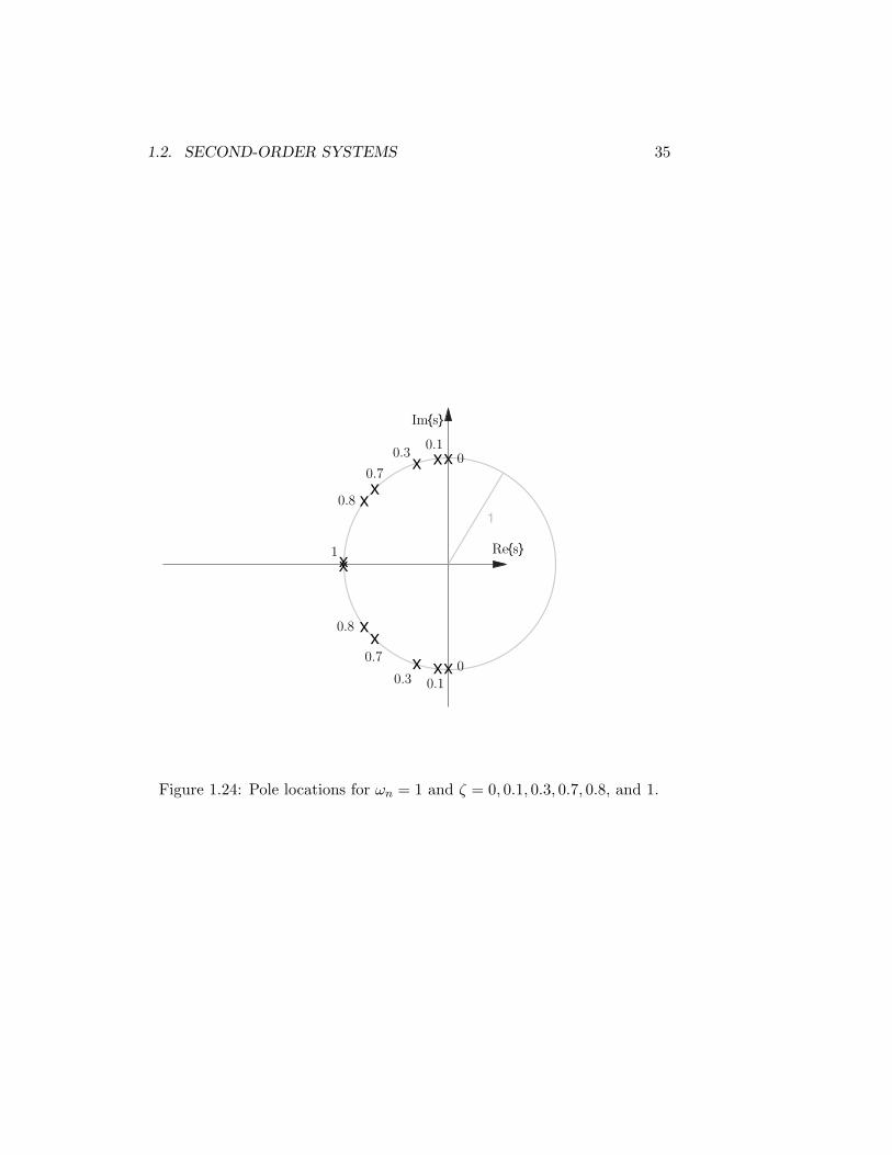
is the damped natural frequency. These pole locations are plotted on the s-plane in Figure 1.23. As shown in the figure, the poles are at a radius from the origin of "n and at an angle from the imaginary axis of ( = sin!1 !. The figure also shows the e!ect of increasing ! and "n. As ! increases from 0 to 1, the poles move along an arc of radius "n from ( = 0 to ( = &/2. As "n increases, the poles move radially away from the origin, maintaining constant angle ( = sin!1 !, and thus constant damping ratio.

To be more specific, the e!ect of ! is shown in Figure 1.24 as ! takes on the values ! = 0, 0.1, 0.3, 0.7, 0.8, and 1.0 for a system with "n = 1.

Now for the details of developing a solution which meets given initial conditions. Since we have s1 = s"

2, the solution (1.49) will be real if c1 = c" 2.


Im{s}

0.10.3

0.7

0.8

1 XX

0.8

0.7

Re{s}

XXX

X X

XXX

X X

0

0

1

0.3 0.1

Figure 1.24: Pole locations for "n = 1 and ! = 0, 0.1, 0.3, 0.7, 0.8, and 1.


With this constraint, as before, the solution simplifies to

x(t) = 2Re{c1e(!$+j"d)t}. (1.54)

As before, we define c1 = # + j$; then the response becomes

x(t) = 2Re{(# + j$)e(!$+j"d)t} (1.55) = 2e!$tRe{(# + j$)(cos "dt + j sin "dt)} (1.56) = 2e!$t(# cos "dt ! $ sin "dt). (1.57)

The position at t = 0 is given by x0 = 2#, and thus to match a specified x0 we require

# = x

2 0 . (1.58)

Taking the derivative with respect to time gives the velocity as

x(t) = !2'e!$t(# cos "dt ! $ sin "dt) + 2e!$t(!#"d sin "dt ! $"d cos "dt) (1.59)

Collecting terms gives

x(t) = 2e!$t ((!'# ! $"d) cos "dt + ('$ ! #"d) sin "dt) , (1.60)

and thus the initial velocity is

v0 = x(0) = 2(!'# ! $"d) (1.61)

Substituting in the earlier result # = x0/2 gives

v0 = 2(! '

2 x0 ! $"d) (1.62)

and thus we can solve for $ as

$ = !(v0

2+ "

'

d

x0) (1.63)

Alternately, the initial condition constant can be expressed in polar notation as we did in the undamped case. That is, let c1 = Mej# , with M = |c1| =

"#2 + $2 and % = arg{c1} = arctan2(#, $). With c1 rep

resented in polar form, the underdamped homogeneous response can be written as

x(t) = 2Re{Mej# e(!$+j"d)t} (1.64) = 2Me!$tRe{ej("dt+#)} (1.65) = 2Me!$t cos("dt + %). (1.66)


This more compact form may be more suitable for some analyses, and is also more helpful when hand-sketching this waveform.

To make things specific, consider the response to initial position x0 = 0 and initial velocity v0 = 1.5 This yields the values # = 0 and $ = !1/2"d. The polar representation is thus M = 1/2"d and % = !&/2. Substituting into either form of the homogeneous solution (1.57, 1.66) gives the response as

1 x(t) = e!$t sin "dt. (1.67)

"d

Note that this solution is valid for all time, and satisfies the initial conditions imposed at t = 0.

The reason for previously defining ' and "d is now more clear since the time response is naturally expressed in terms of these variables. Note that since both ' and "d scale linearly with "n, the response characteristic time-scale decreases as 1/"n. Also note that for a constant initial velocity, the response amplitude decreases with "n. This is so because assuming that m is a fixed value, increasing "n while holding ! constant requires increasing the values of both k and b. Thus, the mass with initial velocity 1 “runs into” a sti!er system, and is returned to rest more rapidly.

This is shown in Figure 1.25 where the response for four values "n = 10, 20, 50, 100 is shown with damping ratio held constant at ! = 0.2. Note that the initial slope of each of the four responses is identical and equal to 1 which, of course, is the initial velocity specified above. The point to retain from Figure 1.25 is that "n sets the response time scale with larger values of "n corresponding to faster time scales.

Viewed another way, the response can be plotted on axes normalized to t# = "nt; this response will then only depend upon the value of !, which determines the relative damping . With time normalized as above, the e!ect of varying values of ! = 0.1, 0.2, 0.5, 0.9 is shown in the plot of the initial condition response (1.67) in Figure 1.26. In this response, the term sin "dt provides the oscillatory part. Multiplying by the term e!$t yields the decaying exponential amplitude on the oscillation seen in the figure. As shown in the figure, as ! (and thus ') approaches zero the response becomes more lightly damped, due to the fact that the exponential envelope decays more slowly.

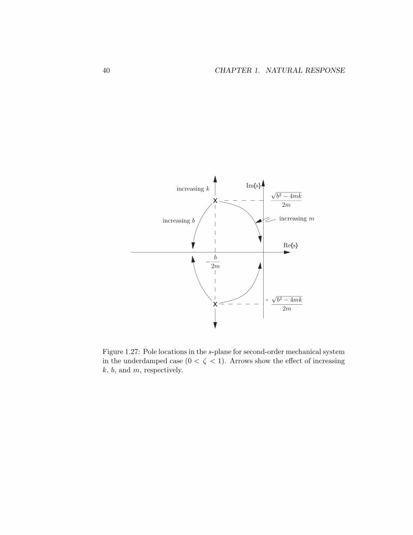
The e!ect of the parameters k, b, and m can also be understood in terms of the s-plane pole locations, as shown in Figure 1.27. Referring to

5This initial condition can be established by an impulse in force Fc of area equal to m N-sec.


0.08

x(t) 0.06

0.04

0.02

0

-0.02

-0.04 0 0.1 0.2 0.3 0.4 0.5 0.6 0.7 0.8 0.9 1

!n = 10

!n = 20

!n = 50

!n = 100

� = 0:2

t

Figure 1.25: Initial condition response (x0 = 0, v0 = 1) for second-order mechanical system in the underdamped case (0 < ! < 1), with varying values of "n = 10, 20, 50, 100, and constant damping ratio ! = 0.2.


1

0.8 x(t)

0.6

0.4

0.2

0

-0.2

-0.4

-0.6

-0.8 0 2 4 6 8 10 12 14 16 18 20

� = 0:1

� = 0:2

� = 0:5

� = 0:9

t0 = !nt

Figure 1.26: Initial condition response for second-order mechanical system in the underdamped case (0 < ! < 1), with varying values of ! = 0.1, 0.2, 0.5, 0.9. Time axis is normalized to t# = "nt.


increasing k Im{s}

X

increasing b

b �2m

X

p�b2 4mk2m

increasing m

Re{s}

-p�b2 4mk 2m

Figure 1.27: Pole locations in the s-plane for second-order mechanical system in the underdamped case (0 < ! < 1). Arrows show the e!ect of increasing k, b, and m, respectively.


k = 100 k = 1000

-0.1

0

0.1

0.2

0.3

0 1 2 3 4 -0.1

0

0.1

0.2

0.3

0 1 2 3 4

k = 3 k = 10

-0.1

0

0.1

0.2

0.3

0 1 2 3 4 -0.1

0

0.1

0.2

0.3

0 1 2 3 4

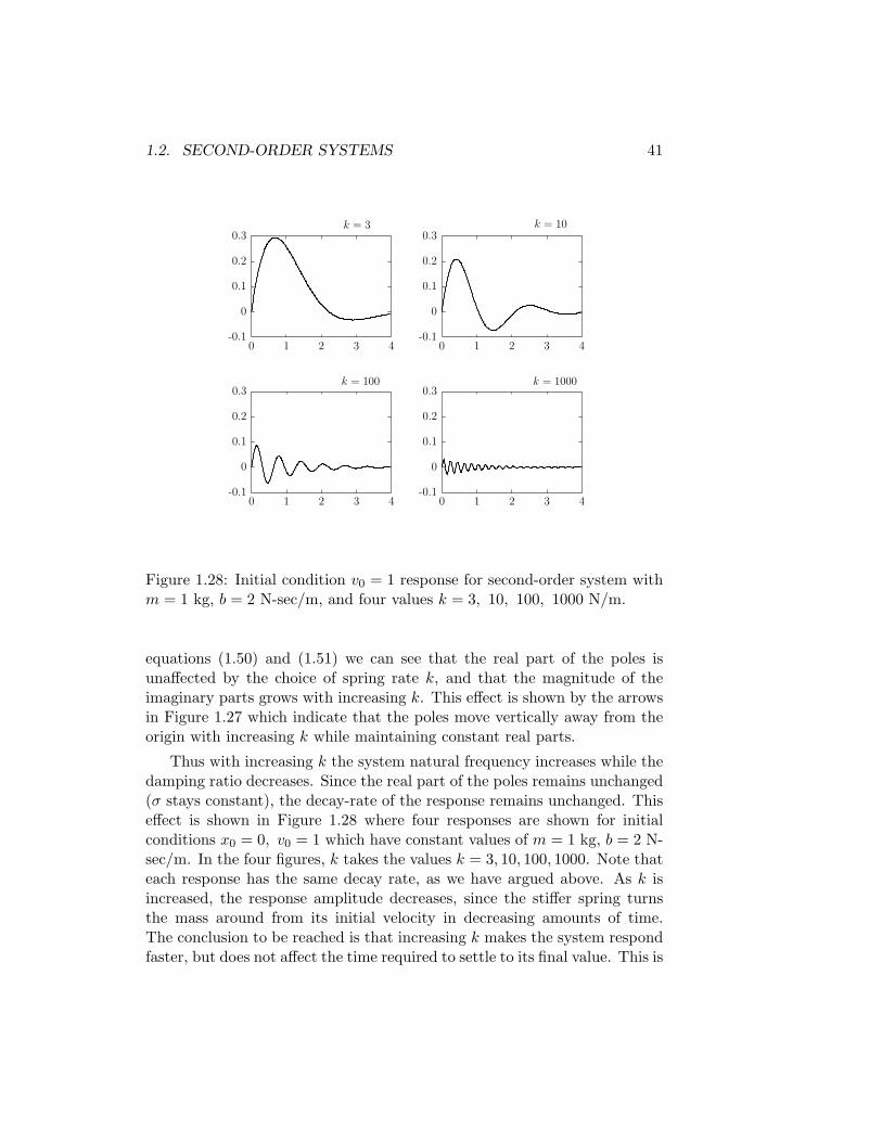
Figure 1.28: Initial condition v0 = 1 response for second-order system with m = 1 kg, b = 2 N-sec/m, and four values k = 3, 10, 100, 1000 N/m.

equations (1.50) and (1.51) we can see that the real part of the poles is una!ected by the choice of spring rate k, and that the magnitude of the imaginary parts grows with increasing k. This e!ect is shown by the arrows in Figure 1.27 which indicate that the poles move vertically away from the origin with increasing k while maintaining constant real parts.

Thus with increasing k the system natural frequency increases while the damping ratio decreases. Since the real part of the poles remains unchanged (' stays constant), the decay-rate of the response remains unchanged. This e!ect is shown in Figure 1.28 where four responses are shown for initial conditions x0 = 0, v0 = 1 which have constant values of m = 1 kg, b = 2 Nsec/m. In the four figures, k takes the values k = 3, 10, 100, 1000. Note that each response has the same decay rate, as we have argued above. As k is increased, the response amplitude decreases, since the sti!er spring turns the mass around from its initial velocity in decreasing amounts of time. The conclusion to be reached is that increasing k makes the system respond faster, but does not a!ect the time required to settle to its final value. This is


-1

-0.5

0

0.5

1

0 10 20 30 40 -1

-0.5

0

0.5

1

0 10 20 30 40

b = .02 b = .2

b = .5 b = 2

-1

-0.5

0

0.5

1

0 10 20 30 40 -1

-0.5

0

0.5

1

0 10 20 30 40

Figure 1.29: Initial condition (x0 = 0, v0 = 1) response for second-order system with m = 1 kg, k = 1 N/m, and four values b = .02, .2, .5, 2 Nsec/m.

an important lesson relating to the design of mechanical structures. Simply sti!ening a structure without adding damping helps in the sense that the amplitude response to disturbances is reduced, but does not help in the sense that the characteristic time required to settle is not reduced.

Referring to equations (1.39) and (1.40) we can see that the natural frequency of the poles is una!ected by the choice of damping constant b, and that ! grows with increasing b. This e!ect is shown by the arrows in Figure 1.27 which indicate that the poles move toward the real axis with increasing b along a circular arc of constant radius "n from the origin. This e!ect is shown in Figure 1.29 where initial condition (x0 = 0, v0 = 1) responses are shown which have constant values of m = 1 kg, k = 1 N/m, and thus "n = 1. In the four figures, b takes the values b = .02, .2, .5, 2 N-sec/m. The conclusion to be reached is that increasing b makes the system better damped, but does not a!ect the natural frequency. It does, however, a!ect the damped natural frequency. For relatively light damping, the damped


0

0.1

0.2

0.3

0.4

0 50 100 150 200 -0.5

0

0.5

1

1.5

0 50 100 150 200

m = 5 m = 1��(critical�damping)

m = 50 m = 500 6

0 50 100 150 200

30

4 20

2 10

0 0

-2 -10

-4 -20 0 50 100 150 200

Figure 1.30: Initial condition response (x0 = 0, v0 = 1) for second-order system with k = 1 N/m, b = 2 N-sec/m, and where m takes the values m = 1, 5, 50, 500 kg.

natural frequency is very close to the natural frequency, and thus the period of oscillation does not change materially in the first three plots. However, as the poles approach the real axis, the damped natural frequency approaches zero, and thus is significantly di!erent from the natural frequency which remains constant as b varied. The last trace in the figure shows the critically damped case, in which "d = 0 and there is thus no oscillation in the response.

The mass m a!ects all the system parameters. As m is increased, the natural frequency decreases, and the damping ratio also decreases. Thus, as m increases, the poles move toward the origin along the arc shown in Figure 1.27. This e!ect is shown in the time-domain in Figure 1.30 where initial condition (x0 = 0, v0 = 1) responses are shown which have constant values of k = 1 N/m, b = 2 N-sec/m, and where m takes the values m = 1, 5, 50, 500 kg. The conclusion to be reached is that as the mass is increased the response characteristic time becomes longer, and simultaneously the response becomes more poorly damped. Note also that the amplitude


Im{s}

�!n Re{s} XX

Figure 1.31: Pole locations in the s-plane for second-order mechanical system in the critically-damped case (! = 1).

of the transient increases strongly with the increase in mass. This e!ect demonstrates why an overloaded car can begin to show poor suspension response.

1.2.5 Critically-damped case

In the critically damped case, ! = 1 and the two poles coincide at s1 = s2 = !"n. These pole locations are plotted on the s-plane in Figure 1.31. The homogeneous solution takes the form

x(t) = c1e s1t + c2tes1t (1.68)

= c1e!"nt + c2te

!"nt (1.69)

where c1 and c2 are real numbers. (Compare this expression to the equivalent result for the undamped case; these look nearly identical, but now the expression is composed of pure real terms.)


In what is now a familiar theme, we use the initial condition specifications to set the values of the parameters c1 and c2 as follows. At t = 0, the position is x0 $ x(0) = c1; this sets the first parameter. Taking the time derivative gives the velocity as

x(t) = !"nc1e!"nt + c2e

!"nt ! "ntc2e!"nt (1.70)

= (c2 ! "nc1 ! "ntc2)e!"nt . (1.71)

At t = 0, the velocity is v0 $ x(0) = c2 ! "nc1. Substituting in with c1 = x0

and rearranging gives the second parameter as c2 = v0 + "nx0. To make things specific, consider the response to an initial position x0 =

0 and initial velocity v0 = 1. The parameters then become c1 = 0 and c2 = 1, and thus the homogenous response is

x(t) = te!"nt . (1.72)

You’ve already seen a plot of this response with "n = 1 in the last panel of Figure 1.29, and the first panel of Figure 1.30. Take a look at these again. For a given "n this is the fastest natural response which exhibits no overshoot as it returns to zero. For this reason, mechanisms and control systems are sometimes tuned for critical damping, or to be only slightly underdamped as it is desirable to have a system which responds quickly, but with little or no overshoot.

1.2.6 Overdamped case

In both the critically damped case and the overdamped case, the description of the pole locations in terms of ! and "n, while mathematically consistent, is not of as great utility as in the underdamped case. Since the poles are real for ! % 1, they can most readily be described in terms of their time constants and viewed as two separate first-order systems. However, for purposes of understanding, we continue the description in terms of the second-order parameters.

In the overdamped case, ! > 1 and the two poles are at separate locations on the real axis: s1 = !(! !

"!2 ! 1)"n and s2 = !(! +

"!2 ! 1)"n. These

pole locations are plotted on the s-plane in Figure 1.32. Note that |s2| > |s1|, and thus the pole at s1 is closer to the origin in the s-plane than s2. In the limit as ! approaches infinity, the root s1 will approach the origin, while the root s2 approaches infinity.6

6As another way of looking at things, it is interesting to note that if the mass m


Im{s}

s2 = s1 =

�(� + p�2 � 1)!n �(� �

p�2 � 1)!n Re{s}

X X

Figure 1.32: Pole locations in the s-plane for second-order mechanical system in the overdamped case (! > 1).


The homogeneous solution takes the familiar form

x(t) = c1e s1t + c2e s2t (1.73)

= c1e!(%!

#%2!1)"nt + c2e

!(%+#

%2!1)"nt (1.74)

where c1 and c2 are real numbers. We use the initial condition specifications to set the values of the pa

rameters c1 and c2 as follows. At t = 0, the position is x0 $ x(0) = c1 + c2. Taking the time derivative in (1.73) gives the velocity as

x(t) = c1s1e s1t + c2s2e s2t . (1.75)

At t = 0, the velocity is v0 $ x(0) = c1s1 + c2s2. Substituting in with c2 = x0 ! c1 and rearranging gives

v0 + x0s2

s2 ! s1

c1 = s2 ! s1

, (1.76)

and c2 = ! .

v0 + x0s1 (1.77)

To make things specific, consider the response to an initial position x0 = 0 and initial velocity v0 = 1. With these initial conditions, the parameters become c1 = !c2 = 1/(s2 ! s1) = 1/(2"n

"!2 ! 1). The response is thus

given by

x(t) = 2"n

"1

!2 ! 1

#e s1t ! e s2t

$ , (1.78)

valid for all time. Plots of this response for "n = 1 and ! = 1, 2, 5, 10 are shown in Figure 1.33.

Note that the response for large ! is approximately first-order with a time constant of !1/s1. This happens because the exponential with the larger pole magnitude decays more quickly than the exponential with the smaller pole magnitude. Thus we see that for stable systems, poles with smaller real part magnitude in the s-plane dominate the time response. As a practical matter, we can ignore in the time response any poles with real parts greater than a factor of 5–10 larger in magnitude than the magnitude of the real part of the dominant poles. Of course, any unstable poles can never be ignored, no matter how far they are from the origin, since their natural response grows exponentially with time.

is allowed to approach zero, and the limits on s1 and s2 are properly taken, then s1

approaches the value !k/b, and s2 approaches infinity. Thus the second-order system in this limit of zero mass properly devolves to the first order case studied in Section 1.1.1.


0

0.1

0.2

0.3

0.4

0 5 10 15 20 0

0.05

0.1

0.15

0.2

0.25

0 5 10 15 20

� = 1 � = 2

� = 5 � = 10

Figure 1.33: Initial condition response for second-order system in the over-damped case, with "n = 1 and ! = 1, 2, 5, 10.

0

0.02

0.04

0.06

0.08

0.1

0 5 10 15 20 0

0.01

0.02

0.03

0.04

0.05

0 5 10 15 20


1.2.7 Canonical second-order form

The results of the previous section are generalizable to other systems which can be modeled with second-order linear constant coe"cient di!erential equations. To summarize these results in a general way:

The canonical form of the second-order homogeneous system (1.41) is repeated here for reference

1 d 2x 2! dx + + x = 0. (1.79)

"2 dt2 "n dt n

Any second-order linear constant coe"cient homogeneous di!erential equation can be written in this form and then the parameters ! and "n read o! by inspection. Then the types of responses plotted in the previous sections for the mechanical system will be directly applicable to many types of physical systems including electrical, thermal, and fluidic as described in the next few sections.

We will also find it helpful to collect here for reference the definition of the real and imaginary parts of the poles. The characteristic equation associated with (1.79) is

1 2! s 2 + s + 1 = 0. (1.80)

"n 2 "n

The roots of this characteristic equation are s = !' ± j"d, where

' = !"n (1.81)

is the attenuation, and "d = "n

"1 ! !2 (1.82)

is the damped natural frequency. Again, these results are applicable to any system which can be expressed in the form (1.79).

The natural frequency "n determines the time-scale of the response; we will assume without loss of generality that "n > 0. Then the damping ratio ! determines much of the character of the natural response:

• If ! < 0, then such a second-order system is unstable in that the natural response grows in time without bound.

• If ! = 0, then such a second-order system is marginally stable in that the natural response is of constant amplitude in time. This is the undamped case studied earlier.


• If ! > 0, then such a second-order system is stable in that the natural response decays exponentially to zero in time. This stable case is further subdivided into three possibilites:

• If 0 < ! < 1, then such a second-order system is underdamped, the poles have imaginary components, and the natural reponse contains some amount of oscillatory component. Lower values of ! correspond with relatively more oscillatory responses, i.e., are more lightly damped.

• If ! = 1, then such a second-order system is critically damped, and the poles are coincident on the negative real axis at a location !"n.

• If ! > 1, then such a second-order system is overdamped, and the poles are at distinct locations on the negative real axis. This case can also be thought of as two independent first-order systems.

1.2.8 Electrical second-order system

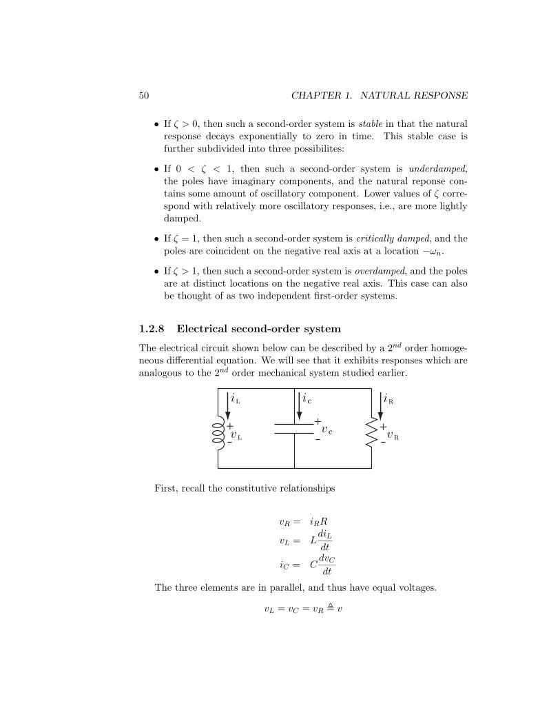
The electrical circuit shown below can be described by a 2nd order homogeneous di!erential equation. We will see that it exhibits responses which are analogous to the 2nd order mechanical system studied earlier.

iL ic iR

++ +v cvL vR

First, recall the constitutive relationships

vR = iRR diL vL = L dt dvCiC = C dt

The three elements are in parallel, and thus have equal voltages.

vL = vC = vR ! v

Documents

1.2 Second-order systems - MIT OpenCourseWare · PDF fileIn the basic linear models considered here, ... SECOND-ORDER SYSTEMS 29 • First, ... exponentials are the natural response