120 - IntechOpencdn.intechopen.com/pdfs/14983/InTech-Critical_state... · 2018-09-25 · The critical state in type II superconductors determines the maximum current the superconductor

0

Critical State Analysis Using Continuous ReadingSQUID Magnetometer

Zdenek Janu1, Zdenek Švindrych2, Ahmed Youssef3 and Lucia Banicová4

1,2Institute of Physics AS CR, v.v.i., Prague3,4Charles University in Prague, Faculty of Mathematics and Physics, Prague

Czech Republic

1. Introduction

The critical state in type II superconductors determines the maximum current thesuperconductor can carry without an energy dissipation. The critical state results from acompetition between the Lorentz force acting on flux lines (quantized vortices), thermalagitation, pinning force, and repulsive interaction between flux lines. The pinning forcelocalizes the flux lines on crystal lattice defects (dislocations, voids or impurities) and favorsglassy state of flux lines, whereas the repulsive interaction between vortices results in a regularflux line lattice. Materials with a strong pinning are called hard superconductors. Suchmaterials are relevant for power application of superconductors: solenoids for high magneticfields or cables for large transport currents. Recently, high temperature superconductor (HTS)materials with the critical current density jc of the order of 100 GA m−2 at zero temperatureand zero applied field were prepared. The second generation of HTS wires (2GHTSC) isconstituted from RE-Ba2Cu3O6+x (YBCO) films. The critical current density is one or twoorders higher than was achieved in Bi2Sr2CaCu2O8+x (BSCCO) round wires or MgB2, Nb-Ti,Nb3Sn, and Nb3Al wires. Unlike BSCCO wires whose performance is lowered by a flux flowat temperature above 35 K the YBCO wires operate even at liquid nitrogen temperature.Another important field of application of superconductors is superconducting electronics.Most of today’s superconducting electronics like superconducting quantum interferometerdevices (SQUIDs), radiation detectors (SIS mixers), etc. are made of Nb, NbN, or HTS films.The flux lines trapped in the superconducting film may deteriorate sensor sensitivity as themoving flux lines generate noise (Wellstood et al., 1987). The above mentioned elucidates aninterest in flux dynamics in thin films, particularly models to a disk and stripe.The critical state is affected by material properties, the wire or sensor geometry (shape),applied current, field, and temperature. Conventionally the critical state is studied (judged)using contact measurements (four probe resistive method) or magnetic measurements (localmagnetization profile or magnetization loops). The latter method eliminates the need forelectrical contacts and allows us to study the response of the critical state to an appliedmagnetic field. Frequency dependent magnetization loops reveal a flux creep or flux flowwhile nonlinear magnetization loops reveal surface or bulk pinning. In order to analyzethese magnetic measurements we need appropriate models. In general, these model representsolution of 3D+t partial differential equations for a magnetic vector potential or flux density.

12

www.intechopen.com

2 Will-be-set-by-IN-TECH

Numerical methods apply to conductors and superconductors with axial symmetry, butotherwise with an arbitrary cross section like cylinders of finite length, thin and thick disks,cones, spheres, and rotational ellipsoids. The specimen may even be inhomogeneous andanisotropic as long as axial symmetry pertains (Brandt, 1998). Complete analytical solutionsare known only for particular geometries and quasistatic behavior of the magnetic flux whenthe problem may be reduced to 2D. Two such examples are thin disk and strip in Bean criticalstate in perpendicular magnetic field.For magnetization loop measurements, one needs a low frequency magnetic field and lowfrequency sensor of the magnetic moment of the sample. The whole system should be of highlinearity, flat frequency and phase dependence - good choice is the superconducting solenoidand SQUID magnetometer. However, commercial SQUID magnetometers are not suitable forsuch measurements because the solenoid operates in a persistent mode during a measurementand settling time (dead time) affects (slows down) the measurement.1 Further, a residual fieldin the high field solenoid causes a nonlinear H(I) dependence. Since the magnetic moment ofthe sample is measured differentially, reciprocating the sample punctuates the measurement.

2. Continuous reading SQUID magnetometer

An operation of a continuous reading SQUID magnetometer (CRSM) with an immobilesample is based on detection coils in a gradiometer arrangement, which are insensitive tothe homogeneous time varying applied magnetic field, but respond to the magnetic sampleplaced in proximity of one of the coils. A spontaneous or induced magnetic moment ofthe sample creates a difference in a magnetic flux in the coils and generates a current in aninput coil of the SQUID. The SQUID thus measures the variations in the magnetic momentof the sample. Since the sample is immobile no noise or disturbances are generated due to asample motion and measurement is not interrupted due to a reciprocating sample or samplepositioning. The applied field is generated by a superconducting solenoid operating in anonpersistent mode.We use SQUID magnetometers in two basic configurations: Standard Sensitivity and HighSensitivity. In a Standard Sensitivity SQUID Magnetometer (SSSM), the superconductingsolenoid, gradiometer, and SQUID are immersed in a liquid helium bath, see Fig. 1. Thesample holder with a sample temperature sensor is placed inside an anticryostat.In a High Sensitivity SQUID Magnetometer (HSSM), the superconducting solenoid,gradiometer, SQUID, and a sample holder with a temperature sensor and heater are placed ina copper vacuum chamber with an inset lead can, see Fig. 1. While the solenoid, gradiometerand SQUID are thermally anchored to the vacuum chamber immersed in a cooling liquidhelium bath, the sample is mounted on a block suspended on a support with a low thermalconductivity.

2.1 Applied field generation

The applied homogeneous field is generated using a superconducting solenoid operatingin the non-persistent mode. The solenoid is wound with a Nb-Ti wire (number of layers)on a coil-former. The solenoid is supplied from a current source driven by a digitalto analog converter (DAC) of a data generation/acquisition card.2 These Σ − Δ DAC

1 Quantum Design.2 National Instruments PC card model PCI-4451.

262 Superconductivity – Theory and Applications

www.intechopen.com

Critical State Analysis Using Continuous Reading SQUID Magnetometer 3

SQUID

superconducting

solenoid

anticryostat

thermometer

resistive heatergradiometer coils

sapphire holder

sample

thermometer

sample holder stick

anticryostat with

exchange gas

isolating space

sample

(a) The standard sensitivity magnetometer.

sapphire sample

holder

SQUID

sapphire

coilformer

gradiometer

upper coil

gradiometer

lower coil

superconducting

solenoid

vacuum

chamber

sample

thermometer

and heater

(b) The high sensitivity magnetometer.

Fig. 1. Schematic drawing of the SQUID magnetometer

have superior linearity and dynamic range. An applied field h(t) may essentially be ofan arbitrary waveform: an AC field superimposed on a DC field for measurement oftemperature dependence of susceptibility, with a linear or sinusoidal sweep for measurementof magnetization loops, pulse or step-like for relaxation measurements, frequency sweep, etc.The waveform is designed numerically.

SSSM HSSM

Field range (Setting resolution) ±25 mT () ±4 mT ()

Frequency range DC - 100 Hz DC - 100 Hz

Temperature range 4.2 - 300 K 4.2 - 150 K

Temperature rate 0.001 - 1 K/min 0.001 - 1 K/min

Sensitivity 7 pA m2 Hz−1/2 5 fA m2 Hz−1/2

Table 1. The parameters of the magnetometers.

Another important property of a SQUID magnetometer is the degree of homogeneity of theapplied magnetic field (both in z and r direction). High homogeneity solenoids generating aDC bias field have the homogeneity of the order of 10−4 over 4 cm (Vrba, 2001).

2.2 Detection system

The detection system includes superconducting flux transformer and the SQUID. Thetransformer comprises of coils in a gradiometric arrangement. Two coils with an oppositewinding (sense) direction and areas S1 and S2 form a first order axial gradiometer which isinsensitive to the homogeneous applied field H0. A balance of the gradiometer, defined as

η = (S1 + S2) · S1/|S1|2 (1)

is η = 0 in an ideal case. In practise, any gradiometer is manufactured with a finite mechanicalprecision and the balance η = 0.0001 may be achieved with a careful construction (Vrba, 2001).

263Critical State Analysis Using Continuous Reading SQUID Magnetometer

www.intechopen.com


An inhomogeneous applied field and imperfect gradiometer balance result in a crosstalk ofthe field to the SQUID and reduce a dynamic range of the CRSM. In SSSM a compensationcoil wound on an upper part of the solenoid and supplied with an adjustable current derivedfrom the solenoid supply current minimizes crosstalk. A careful design and constructionkeeps down deformation of the field affected by a proximity of magnetic or superconductingmaterials (solder) and frequency dependent eddy currents in metallic (nonsuperconducting)parts.The magnetic moment of the sample is

m =12

∫

V(r × j) d3r. (2)

A vector potential of the induced or spontaneous magnetic moment m of the sample is

A = μm × r

r3 . (3)

The magnetic flux in the pickup coil is

Φ =∮

ΓA · dl, (4)

where Γ is the coil circumference. The SQUID indicates difference in the flux in an upper andlower coil, ΔΦ = Φupper − Φlower, and thus the SQUID output voltage is proportional to aprojection of the measured magnetic moment on a gradiometer axis, m(t) ∝ ΔΦ(t).Since the detection system is superconducting, the output voltage m(t) is proportional to themagnetic moment of the sample and not to a rate of change of the magnetic moment like incase of induction magnetometers (ac susceptometer (ACS) or vibrating sample magnetometer(VSM)).Both the SSSM and HSSM use bulk Nb SQUID of the Zimmerman type operating at the rffrequency of about 40 MHz. The Josephson junction is a point contact type in the SSSM andthin film bridge in the HSSM. Both SQUIDs have an equivalent input flux noise density of theorder of 10−4 Φ0 Hz−1/2 in a white noise region (> 1 Hz) and range ±500 Φ0 limited by a slewrate 104 Φ0/s.3

A shielding of an external dc and time varying electromagnetic field originating from an earthmagnetic field and man-made sources is necessary to utilize the extraordinary sensitivity ofthe SQUIDs. The shielding is ensured by a soft magnetic materials (the cryostat is placedinside the shielding) and superconducting shielding (Tsoy et al., 2000).

2.3 Sample mounting and temperature reading and control

In SSSM a sample is glued on a bottom surface of a cylindrical sapphire holder using a varnishor grease. A sample temperature sensor, the Si or GaAlAs diode4, is mounted on the uppersurface. The sapphire holder is connected to a (nonmagnetic, nonconducting) polyethylenestraw that extends a thin wall stainless tube suspended in an anticryostat. Another Si diode

3 iMAG 303 SQUID: The equivalent input noise for the standard LTS SQUID system is less than 10−5 Φ0

Hz−1/2, from 1 Hz to 50 kHz in the ±500 Φ0 range. The response is flat from DC to the 3 dB points,slow slew mode 500 Hz (- 3 dB), normal slew mode 50 kHz (- 3 dB). The input inductance of the LTSSQUID is 1.8 × 10−6 H.

4 Lake Shore or CryoCon


www.intechopen.com


temperature sensor measures temperature of the anticryostat to facilitate better closed-looptemperature control. Two section resistance wire (constantan) heater is wound around the topand bottom part of the anticryostat to ensure uniform warming. Heat is removed from thesample by a 4He gas at atmospheric pressure.In HSSM the sample is mounted on the upper surface of the sapphire holder. The holder isembedded in a copper block whose temperature is measured using the Si diode sensor. Theblock is heated using a resistance wire heater and suspended on a low thermal conductivityfibreglass support which removes heat to liquid 4He bath. The sample is in vacuum.In both magnetometers, a temperature controller5 connected to the computer regulatestemperature with relative stability of 10 ppm and 1 ppm in SSSM and HSSM, respectively,and controls cooling or warming with rate from 1 mK/min to 10 K/min.

2.4 Measurement modes

The magnetometers are designed for measurements of: i) temperature dependence of aresponse to fixed AC and DC applied magnetic field (temperature dependence of thesusceptibility); ii) response to field sweep at fixed temperature and AC field (magnetizationloops and AC susceptibility); iii) relaxation of a DC magnetic moment (after applied fieldpulse or step) as a function of time or temperature; iv) frequency dependence at a fixed DCfield and temperature. Additional measurement modes require only a software change.

2.5 Data acquisition

The dynamic range of the SQUID is extraordinary, the range of ±500 Φ0 and spectral fluxnoise density of 10−4 Φ0 Hz−1/2 represent output voltage range ±10 V and voltage noisedensity 10 μV Hz−1/2, a range of 7 orders (140 dB).6 The frequency response is flat both in afrequency and phase. In slow slew mode the -3 dB point is 100 Hz. The SQUID output signalm(t) falls into an audio range and thus may be easily digitized in "CD" quality as well as thesignal of the applied field H(t), recorded on a hard disk, and digitally processed in real time.7

Processed data file includes temperature readings.

2.6 AC susceptibility measurement (calculation)

Let the time varying applied AC magnetic field is

H (t) = Hac cos (2π f0t) = HacRe exp (i2π f0t) , (5)

where Hac is the amplitude and f0 is the frequency of the applied field. The complex ACsusceptibility of the sample is

χn =M (n f0)

HacV, (6)

5 CryoCon model 346 This applies to rf-SQUIDs. The flux noise density in DC SQUIDs is lower, 10−6 Φ0 Hz−1/2,

corresponding voltage noise density 0.1 μV Hz−1/2, and dynamic range of 9 orders (180 dB).7 We use the National Instruments PC cards model PCI-4451 with Σ − Δ digital to analog and analog

to digital converters for a digital signal generation and acquisition (two input channels with 16 bitresolution, frequency range from 0 (true DC) to 95 kHz, and sampling rate up to 204.8 kS/s).


www.intechopen.com


where n denotes harmonics and M(n f0) are the Fourier components of the magnetic momentm(t). Higher harmonics of the complex susceptibility appear in the case of a nonlinearresponse to the applied field. Usually the susceptibility is normalized to a volume V (or mass)of the sample. Using the susceptibility, the magnetization loops are

M (H (t)) = ∑n

χn Hac exp (ni2π f0t) , (7)

A common way to measure the AC susceptibility is to detect a signal of the magnetic momentusing a phase sensitive lock-in amplifier, preferably a two phase instrument indicating bothreal and imaginary part of the AC susceptibility, and drive the AC field using a signalgenerator. The conventional analog lock-in amplifier multiplies the input signal m(t) by asquare wave r(t) derived from a reference signal H(t) and integrates the product. The DCoutput are in-phase and out-of-phase components

ReM( f0) =4

πτ

∫ t

t−τ

[

∞

∑n=1

1n

sin(nπ

2) cos

(

n2π f0t′)

]

m(t′)dt′, (8)

ImM( f0) =4

πτ

∫ t

t−τ

[

∞

∑n=1

1n

sin(

n2π f0t′)

]

m(t′)dt′, (9)

where n is odd and τ is the averaging time constant. Since the reference signal r(t) is a squarewave, the DC output is proportional not only to the Fourier component of the first harmonicbut also to 1/3 of third, 1/5 of fifth, etc. Evidently, this way of signal processing is not suitablefor the measurement of a nonlinear response. One can apply input filters that sufficientlysuppress third and higher odd harmonics, but remain unaffected the fundamental frequency.However, suitable tunable filters are complex and expensive.In the digital signal processor (DSP) lock-in amplifiers the signal is filtered with a simpleanti-aliasing filter and digitized by over-sampling ADC with subsequent digital filtering. TheDSP chip then synthesizes digital reference sine (and cosine) wave at the reference frequencyn f0 and multiplies the signal by this reference. After multiplication, stages of digital low-passfiltering are applied to average over the signal period. The DSP lock-in amplifier generatesthe true rms values of the complex Fourier components of M( f0) or nth harmonic M(n f0):

M (n f0) =1

NΔt

N−1

∑k=0

m (tk) exp (ni2π f0tk) , (10)

where Δt = tk − tk−1 is the sampling interval and NΔt is averaging time. However,commercial DSP lock-in amplifiers provide only components at single frequency. Hence,unless successive measurements of the harmonics are done, one needs an extra instrumentfor the each additional harmonic.With computational power of today’s processors in personal computers (PC) and datageneration/acquisition hardware the problem as a whole may be solved much moreeffectively. The single PC card, with essentially the same ADC as are used in the DSP lock-inamplifier, substitutes for the generator and lock-in amplifiers. Since the DACs generatingthe applied field and ADCs sampling m(t) and H(t) use the same clock, synchronization isguaranteed. In reality, an approach using a direct digital signal generation, acquisition, andprocessing is more cost effective and less time consuming.


www.intechopen.com


The nth harmonic of the AC susceptibility is given by generalized Eq. 6,

χn =M(n f0)

Hac exp(niϕ), (11)

where complex Hac exp(niϕ) ≡ |H( f0)| exp(ni argH( f0)) takes into account a phase of theFourier component of the applied field H( f0), i.e. a time shift between a Fourier transformeddata segment and cosine field. The M( f ) and H( f ) spectra are computed using a discrete fastFourier transform (FFT) of real data arrays m(tk) and H(tk).

Ml ≡N−1

∑k=0

m(tk) exp (i2πkl/N) , (12)

(the same holds for H(t) ⇔ H( f )), where N is the transform length (Press et al., 1992). Spectraof the complex amplitudes M( f ) and H( f ) are calculated for frequencies lΔ f , Ml ≡ M(lΔ f ).With an applied FFT algorithm N must be a power of 2, FFT is computed in N log N

operations, and Δ f = fs/N, where fs = 1/Δt is the sampling frequency.8 Unlike the DSPlock-in amplifiers, where another instrument performing N operations to process NΔt longrecord is need for each measured harmonic, here the whole frequency spectrum from DC tof /2 is computed with only N log N operations using the single instrument. Computation timetakes few ms.Strictly speaking, the measurement of temperature dependence of the susceptibility representsa continuous measurement of magnetization loops at slowly varying temperature. Sincethe input signals are recorded as well as temperature readings, various time domain andfrequency domain filters may be applied thereupon. The magnetization loops may beprocessed using different time windows (for example to remove a linear trend in m(t)) ordifferent averaging times.

3. Critical state in type II superconductors

3.1 Vortex matter

Type II superconductors, ie. those with λ/ξ > 2−1/2, where λ is the flux penetration lengthand ξ is the coherence length of a superconducting order parameter, remain superconductingeven in a high magnetic field due to lowering of their energy by creating walls between normaland superconducting regions. Consequently, flux lines (vortices) with a normal core of aradius of ≈ ξ, where the order parameter vanishes, and persistent current circulating aroundthe core and decaying away from the vortex core at distances comparable with λ are createdat sample edges and penetrate into an interior of the superconductor. The vortex is a linear (inthree dimensions) object which is characterized by a quantized circulation of the phase of theorder parameter around its axis and carries a single quantum of the magnetic flux Φ0 = h/2e.The superconductor penetrated with the flux lines is called to be in a mixed state. A repulsiveinteraction between the flux lines eventually forms flux line bundles and consecutively a flux

8 Let us take N = 214 (16 K samples), easy for real time processing on a common PC. With fs = 6.4 kS/sthe Δ f = 0.390625 Hz. A right choice for the AC field frequency f0 is an integer multiple of Δ f . Forexample, with f0 = 4Δ f = 1.5625 Hz, one period of the AC field is represented by 4 K samples. In thiscase the 16 K FFT means averaging over 4 periods (2.56 s) of the AC field. If the 16 K data are shiftedby 4 K and a void part is replaced with samples of the latest read period, the spectra are averaged over2.56 s and updated in 0.64 s interval. The index of the nth harmonics amplitude is l = n4.


www.intechopen.com


line lattice. In increasing applied field the flux lines enter into the superconductor when themagnetic field exceeds the lower critical field Hc1 ≈ Φ0/μ0λ2. Type II superconductorsexperience a second-order phase transition into a normal state at the upper critical fieldHc2 ≈ Φ0/μ0ξ2. In type I superconductors this transition is a first-order in a nonzero field.

3.2 Pinning and surface barrier

In a real type II superconductor there are always crystal lattice distortions, voids, interstitials,and impurities with reduced superconducting properties. The superconducting orderparameter is either reduced or suppressed completely, just as within a vortex core. Thatimplies that such defects are energetically favorable places for vortices to reside and thevortices will be pinned in the potential of these so-called pinning centers. The efficiency ofsuch a pinning center is at its maximum if its size is of the order of the coherence length ξ. Ifthere is almost no pinning, flux flow occurs (Bardeen, 1965). On the other hand, when there isfinite pinning, flux creep of a vortex bundles takes place (Anderson, 1962; 1964). The bundlesize is determined by the competition between pinning and the elastic properties of the vortexlattice.An edge or surface barrier may oppose a flux entry into the sample (Beek et al., 1996). Asurface barrier arises as a result of the repulsive force between vortices and the surfaceshielding current. The first example is Bean-Livingston barrier, which is a feature of flattype II superconductor surfaces in general and is related to a deformation of the vortex at thesurface (mirror vortex). The second example is the edge-shape barrier, which is a geometriceffect related to the distribution of the Meissner shielding current density in non-ellipsoidalsamples.When an increasing magnetic field is initially applied, flux cannot overcome the barrier, andM = −H. At the field of the first flux penetration Hp, the magnetic pressure is sufficiently highto overcome the barrier. If there is no pinning, vortices will now distribute themselves throughthe sample in such a way that the bulk current is zero and vortex density is homogeneous.

3.3 Flux line dynamics

When the superconductor is carrying a bulk transport or shielding current density j theflux lines experience a volume density of the driving Lorentz force fL = j × B, where B

is the flux density inside the flux line. When the Lorentz force acting on the flux lines isexactly balanced by the pinning force density, i.e. FL = Fp, the current density is called thedepinning current density, jc. Under this force the flux lines may move through the crystallattice and dissipate energy. In this case the electrical losses are no longer zero. In an ideal(homogeneous) type II superconductor there is nothing to hinder the motion of flux lines andthe flux lines distribution is homogeneous. The flux lines can move freely, which is equivalentto a vanishing critical depinning current density jc. On the other hand, the non-dissipativemacroscopic currents are the result of the spatial gradients in the density of flux lines or dueto their curvature. This is possible only due to the existence of pinning centers, which cancompensate the Lorentz force.The moving flux lines dissipate energy by two effects which give approximately equalcontributions: (a) eddy currents that surround each moving flux line and have to pass throughthe vortex core, which in the model of Bardeen and Stephen is approximated by a normalconducting cylinder (normal currents flowing through the vortex core) (Bardeen, 1962); (b)


www.intechopen.com


Tinkham’s mechanism of a retarded recovery of the order parameter at places where thevortex core has passed (Tinkham, 1996).In general, the current density in type II superconductors can have three different origins: (a)Surface currents within the penetration depth λ. In the Meissner state the current passingthrough a thick superconductor is restricted to a thin surface layer where the magneticfield can penetrate. Otherwise the magnetic field due to the current would exist inside thesuperconductor; (b) A gradient of the flux-line density; (c) A curvature of the flux lines.A flux line motion is discouraged (inhibited) by pinning of individual flux lines, their bundlesor lattice. In cases of flux flow and flux creep, the vortices are considered to move in anelastic bundle. With discovery of HTS, however, more complex forms of vortex motion areconsidered. When the driving force is small, the vortices move in a plastic manner - plasticflow where there are channels in which vortices move with a finite velocity, whereas in otherchannels the vortices remain pinned (Jensen, 1988). Thus, between moving channels and staticchannels there are dislocations in the flux lattice. With further increasing driving current,vortices tend to re-order. Through dynamic melting, a stationary flux lattice changes into amoving flux lattice via the plastic flow (Koshelev & Vinokur, 1994).If pinning is efficient the critical depinning current density jc becomes high and the materialis interesting for applications. The properties of the flux line lattice and the pinning propertiesare important for applications; on the other hand they are complex and interesting topics ofcondensed-matter physics and materials science.

3.4 Equation of motion of vector potential

In general, computation of magnetization loops represents a full treatment of a nonlinear 3Dproblem described by a partial differential equation for a vector potential

∂A

∂t= D∇2A, (13)

where D is the diffusivity. Due to an axial symmetry or for a long sample in a parallel field,the problem may reduce to 2D and the current density j, vector potential A, and electric fieldE are parallel to each other and have only a y or φ component (applied field is parallel to z

axis) (Brandt, 1998). The magnetization loops are obtained solving Eq. 13 using specializedsoftware packages or directly by the time integration of the nonlocal and nonlinear diffusionequation of motion for the azimuthal current density. A long cylinder or slab in parallel fieldor thin circular disk and strip in an axial field are 1D problems. The flux density and electricfield are B = ∇× A and E = −∂A/∂t, respectively.In the normal (nonsuperconducting) state with an ohmic conductivity σ is D = 1/μ0σ =m/μ0ne2τ. In Meissner state the diffusivity is the pure imaginary D = iωm/μ0nse2 with alinear frequency dependence, where ns is the superconducting condensate density.In an inhomogeneous type II superconductor with flux pinning the electric field is given bynonlinear local and isotropic resistivity ρ(j). A material law E(j) reflects a flux line pinning.In case of a strong pinning E(j) is zero up to the critical depinning density jc at which electricfield raises sharply. A power law voltage current relation

E(j) = Ec|j/jc|nj/j = ρc|j/jc|

n−1j, (14)


www.intechopen.com


where j = |j|, is observed in numerous experiments (Brandt, 1996). From the theories on(collective) creep, flux penetration, vortex glass picture, and AC susceptibility one obtains theuseful general interpolation formula

U(J) = U0(jc/j)α − 1

α. (15)

Here U(j) is a current-dependent activation energy for depinning which vanishes at thecritical current density jc, and α is a small positive exponent. In the limit α → 0 one has alogarithmic dependence of the activation energy U(j) = U0 ln(jc/j), which inserted into anArrhenius law yields

E(j) = Ec exp(

−U (j)

kBT

)

= Ec

(

j

jc

)U0/kBT

. (16)

When we compare Eq. 16 with Eq. 14 the exponent is n = U0/kBT. For α = −1 the Eq.15 coincides with the result of the Kim-Anderson model, E(j) = Ec exp[(U0/kBT)(1 − j/jc)],(Blatter et al., 1994). For α = 1 one gets E(j) = Ec exp[(U0/kBT)(jc/j − 1)].In general, the Ec and activation energy U in Eq. 16 depend on the local induction B(r) andthus also α(B, T) and jc(B, T) depend on B.With E = −∂A/∂t and Eq. 14 one obtains for the diffusivity in Eq. 13

D(j, jc, U0, T) =1

μ0

∂E

∂j=

1μ0

Ec

jc

(

j

jc

)U0/kBT−1=

ρc

μ0

(

j

jc

)U0/kBT−1. (17)

Power-law electric field versus current density (Eq. 14) induces:i) An Ohmic conductor behavior with a constant resistivity ρ = E/j for U0/kBT = 1. Thisapplies also to superconductors in the regime of a linear flux flow or thermally activatedflux flow (TAFF) at low frequencies with flux-flow resistivity ρ f = ρnB/μ0Hc2, known asthe Bardeen-Stephen model. The diffusivity D is large and vector potential profiles are timedependent. The magnetization loops have a strong frequency dependence, as well as thesusceptibility, and the AC susceptibility has only fundamental component independent onthe AC field amplitude (Gömöry, 1997).ii) Flux creep behavior for 1 ≪ U0/kBT < ∞. The magnetization loops have a weak frequencydependence, as well as the AC susceptibility which has higher harmonics and is dependenton the AC field amplitude.iii) Hard superconductors with strong pinning for U0/kBT → ∞. In this case the fluxdynamics is quasistatic, described by a Bean model of the critical state with D = 0 for |j| < jcand D → ∞ for |j| = jc. The magnetization loops are frequency independent, as well as the ACsusceptibility which has higher harmonics and strongly depends on the AC field amplitude.A general solution of Eq. 13 represents time dependent vector potential profiles whichdynamics covers a viscous flow, diffusion (creep), and quasistatic (sand pile like) behavior.The resistivity generated by the flux creep is Ohmic in the low-driving force limit.

3.5 Analytically solvable models

3.5.1 Normal state with ohmic conductivity and flux flow state

In normal state with an ohmic conductivity σ = ne2τ/m the diffusion constant is D =1/μ0σ = ωδ2, where ω is the angular frequency of the applied AC field and δ = (2μ0ωσ)−1/2


www.intechopen.com


is the normal skin depth. In this case the analytical solutions to Eq. 13 are known for aninfinitely long cylinder and slab in a parallel field, cylinder in a perpendicular field, and sphere(Brandt, 1998; Khoder & Couach, 1991; Lifshitz et al., 1984).With an increasing ratio δ/R or δ/d, where and R is the radius of the cylinder or sphere and 2d

id the slab thickness, a sample changes from a diamagnetic (but lossy) at δ ≪ R, to absorptiveat δ ≈ R, and to transparent for applied field at δ ≫ R. The magnetization loops M(H)are ellipses which major axis lies on H axis of H − M diagram for transparent medium andgradually turns to −π/4 direction for diamagnetic medium. The susceptibility as a functionof (δ/R)2 is shown in Fig. 2.In a limit of low frequencies when the skin depth δ ≫ R, d and the sample is transparent forAC field the first terms in series expansion of the susceptibility are (up to a shape dependentmultiplication factor)

Reχ ≈ −(

R2μωσ)2

(18)

Imχ ≈(

R2μωσ)

, (19)

and Reχ ≪ Imχ. A measurement of χ yields contactless estimation of the electricalconductivity σ.In a linear or thermally activated flux flow state as the applied field approaches the uppercritical field Hc2, the flux density in the superconductor B → μ0Hc2 and the flux flowresistivity ρ f smoothly transforms to ρn = 1/σ

ρ f

ρn≈

B

μ0Hc2(20)

as the phase transition between a mixed state and normal state is of second order (BardeenStephen model) (Bardeen, 1965). Flux flow resistivity may be estimated using Eq. 19.

3.5.2 Meissner state

At initial magnetization the superconductor is in Meissner state in field lower that Hc1. Inthis case the diffusivity is pure imaginary D = iωλ2, where the flux penetration length isλ = (μ0nse2/m)−1/2. The susceptibility of an infinitely long cylinder and slab in a parallelfield, cylinder in a perpendicular field, and sphere is obtained like for normal state butreplacing (1 + i)/δ with i/λ (Brandt, 1998; Khoder & Couach, 1991; Lifshitz et al., 1984). Thesusceptibility as a function of (λ/R)2 is shown in Fig. 2.In a weak field, low temperature part of the susceptibility (T/Tc < 0.5) is proportional to theflux penetration length

Reχ(T) = −1 + aλ(T)/R. (21)

A measurement of temperature dependence λ(T) allows us to distinguish differentpairing symmetries. While in conventional superconductors with an isotropic gapthe quasiparticle excitations rise with increasing temperature as exp(−Δ/kBT), innonconventional superconductors, for example HTS, a temperature dependence is power-law.As far as we know, it fails to fit experimental χ(T) at T → Tc even for well known λ(T), atlow temperatures.


www.intechopen.com


-1.2

-1

-0.8

-0.6

-0.4

-0.2

0

0.2

0.4

0.6

1E-06 1E-05 0.0001 0.001 0.01 0.1 1 10 100 1000

(d/R)2

Su

sc

ep

tib

ilit

yReX sphere

ImX sphere

ReX slab

ImX slab

SC sphere

SC slab

SC cylinder

Fig. 2. The dependence of the complex AC susceptibility of a sphere and slab in a normal(ohmic) state in a parallel field on (δ/R)2 ∝ ρn and of the sphere, slab and cylinder inMeissner state on (λ/R)2 ∝ 1/ns. In an ohmic state an absorption peak appears on Imχ, theheight of which is characteristic of sample shape.

3.5.3 Bean critical state

The Bean model of the critical state is the case of a strong pinning when the flux densityvariation is quasi-static (frequency independent) in a slowly varying applied magnetic fieldand the flux density profile changes only when induced shielding current density reaches thecritical depinning current density j = ±jc. An electric field is induced when the flux densitychanges. In a slab the flux density profile is linear |∂Bz(x)/∂x| = μ0 jc in flux penetratedregions and |B| = 0 in untouched regions. The model assumes lower critical field Hc1 → 0,surface barrier Hbarrier → 0, and field independent critical depinning current density jc, i.e.jc(B) is constant (Bean, 1964).Analytical solutions for magnetization loops are known for an infinitely long slab or cylinderin a parallel field (Goldfarb, 1991) and thin disk (Clem & Sanchez, 1994; Mikheenko &Kuzovlev, 1993) or strip (Brandt, 1993) in a perpendicular field. In these cases the 3D partialdifferential equation (PDE) Eq. 13 reduces to a time independent 2D PDE due to sample shapesymmetry.The model to the disks was work out by Clem and Sanches who improved and correctedformer model worked out by Mikheenko and Kuzovlev (Clem & Sanchez, 1994). The modelis restricted to slow, quasistatic flux changes for which the magnitude of the electric field E

induced by the moving magnetic flux is small in comparison with ρ f jc, where ρ f is the fluxflow resistivity. Under these conditions, the magnitude of the induced current density is closeto the critical depinning current density. The validity of the model is restricted for d ≪ R,d ≥ λ or if d < λ, that Λ = 2λ2/d ≪ R, where λ is the flux penetration length and Λ is the2D screening length.In the case of the infinitely long (or sufficiently long) sample (slab or cylinder) in parallelapplied field the shielding current density is at a surface parallel with applied field,

μ0 jφ = −∂Bz/∂r (22)

while in case of the sufficiently thin sample (disk or strip) in perpendicular applied field


www.intechopen.com


μ0 jφ = ∂Br/∂z, (23)

the shielding current appears simultaneously everywhere over the sample cross-section uponapplication of the field, and decreases everywhere simultaneously after a decrease of thefield (Beek et al., 1996). The complete magnetic hysteresis loop can be obtained from thefirst magnetization curve, which is almost the same for the above cases. The hysteresis loopdevelops from the thin lens-shaped to parallelogram as the Hac is increased or jc decreases.The lens shape corresponds to partial penetration of the magnetic flux while the parallelogramoccurs when the magnetization is saturated.The component of the magnetization parallel to the applied periodically time varying fieldH(ϕ) = Hac sin ϕ is

M∓ = ∓χ0HacS(

Hac

Hd

)

± χ0 (Hac ∓ H) S(

Hac ∓ H

2Hd

)

, (24)

where M− and M+ are for decreasing and increasing applied field, respectively (Clem &Sanchez, 1994). A characteristic field Hd = djc/2, where d is the disk thickness and jc isthe critical depinning current density (temperature dependent). The function S(x) is definedas

S (x) =1

2x

[

arccos(

1cosh x

)

+sinh |x|

cosh2 x

]

. (25)

3.5.4 Mapping of model susceptibility to experimental susceptibility

The model AC susceptibility is calculated for magnetization loops Eq. 24 using Eq. 11, i.e.in the same way as the experimental susceptibility (Youssef et al., 2009). To map the modelsusceptibility χ(Hac/Hd) to the experimental temperature dependent susceptibility χ(T) weuse a proportionality of the characteristic field to the critical depinning current density, Hd =djc/2, and a fact that experimentally observed temperature dependence, jc(T) = jc(0)(1 −T/Tc)n, is power-law. Further, we need an inverse function for jc(T) and insert the amplitudeof the applied field. Let us take

jc(T)

jc(0)=

Hd(T)

Hd(0)=

(

1 −(

T

Tc

)m)n

. (26)

Relation between temperature T and ratio Hd/Hac, i.e. experimental and model susceptibility,is obtained using inverse function for Eq. 26 and multiplying both the numerator anddenominator, Hd/Hd(0), by Hac

(

T

Tc

)

model

=

(

1 −(

Hac

Hd(0)Hd

Hac

)1/n)1/m

. (27)

We have four free parameters c ≡ Hac/Hd(0), n, m, and Tc to match the model andexperimental susceptibility

⎡

⎣

(

1 −(

cHd

Hac

)1n

)

1m

, χ

(

Hd

Hac

)

⎤

←→

[

T

Tc, χ(T)

]

. (28)


www.intechopen.com


When we find c, n, m, and Tc, the zero temperature critical depinning current density is

jc(0) = 2Hac/cd (29)

and its temperature dependence is given by Eq. 26.

-0.06

-0.05

-0.04

-0.03

-0.02

-0.01

0

0.01

0.02

-3 -2.5 -2 -1.5 -1 -0.5 0

-(H p /3H ac )1/3

, -(H d /H ac )1/2

3rd

harm

on

ic o

f ac s

uscep

tib

ilit

y

ReX(3) Cylinder

ImX(3) Cylinder

ReX(3) Disk

ImX(3) Disk

(a) The third harmonic of the AC susceptibility.

-0.015

-0.01

-0.005

0

0.005

-3 -2.5 -2 -1.5 -1 -0.5 0

-(H p /3H ac )1/3

, -(H d /H ac )1/2

5th

harm

on

ic o

f ac s

uscep

tib

ilit

yReX(5) Cylinder

ImX(5) Cylinder

ReX(5) Disk

ImX(5) Disk

(b) The fifth harmonic of the AC susceptibility.

Fig. 3. Differences in the harmonics of AC susceptibility for models of cylinders and disks.The susceptibility is plotted versus "model temperature" given by Eq. 27 (Youssef et al.,2009). Here Hp is the characteristic field for a cylinder, Hp = Rjc.

3.5.5 Interpretation of complex AC susceptibility

The real part of the fundamental AC susceptibility represents a magnetic energy of thesample stored in the diamagnetic shielding current. The imaginary part of the fundamentalsusceptibility is related to losses caused by resistive response (dissipation).In normal state or in flux flow state the AC susceptibility is a function of appliedfield frequency, conductivity (resistivity), and temperature but is independent of the fieldamplitude. On the other hand, in a case of strong pinning the AC susceptibility is a functionof the applied field amplitude, critical depinning current density, and temperature but isindependent of frequency. Nonlinear dependence of the sample magnetization on appliedfield amplitude generates harmonics of AC susceptibility. Their behavior is characteristic fora given sample shape. Due to a symmetry of the magnetization loops, M(H) = −M(−H),the coefficients of even harmonics of the AC susceptibility are zero.

4. Experimental results on critical state in type II superconductors

Recently developed second generation of the high temperature superconductor wires on thebasis of YBaCuO films and Nb films for superconductor electronics production representproper materials to study models to the critical state in hard superconductors.


www.intechopen.com


4.1 Materials

The Nb film of thickness of 250 nm was deposited by a dc magnetron sputtering in Ar gason 400 nm thick silicon-dioxide buffer layer which was grown by a thermal oxidation of asilicon single crystal wafer (May, 1984). The film is polycrystalline with texture of a preferredorientation in the (110) direction and is highly tensile. Grain size is about 100 nm. The squaresamples of 5 × 5 mm2 in dimensions were cut out from the 3-inch wafer.Second-generation high temperature superconductor wire (2G HTS wire) consists of a 50 μmnonmagnetic nickel alloy substrate (Hastelloy), 0.2 μm of a textured MgO-based buffer stackdeposited by an assisting ion beam, 1 μm RE-Ba2Cu3Ox superconducting layer SmYBaCuOdeposited by metallo-organic chemical vapor deposition, and 2 μm of Ag, with 40 μm totalthickness of surround copper stabilizer (20 μm each side) .9 The sample is cut into 4 mm longsegment of 4 mm wide wire.

4.2 Estimation of the critical depinning current density and its temperature dependence

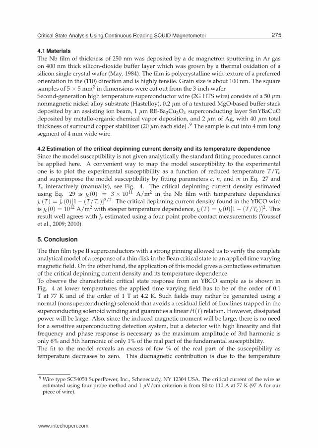
Since the model susceptibility is not given analytically the standard fitting procedures cannotbe applied here. A convenient way to map the model susceptibility to the experimentalone is to plot the experimental susceptibility as a function of reduced temperature T/Tc

and superimpose the model susceptibility by fitting parameters c, n, and m in Eq. 27 andTc interactively (manually), see Fig. 4. The critical depinning current density estimatedusing Eq. 29 is jc(0) = 3 × 1011 A/m2 in the Nb film with temperature dependencejc(T) = jc(0)[1 − (T/Tc)]3/2. The critical depinning current density found in the YBCO wireis jc(0) = 1012 A/m2 with steeper temperature dependence, jc(T) = jc(0)[1 − (T/Tc)]2. Thisresult well agrees with jc estimated using a four point probe contact measurements (Youssefet al., 2009; 2010).

5. Conclusion

The thin film type II superconductors with a strong pinning allowed us to verify the completeanalytical model of a response of a thin disk in the Bean critical state to an applied time varyingmagnetic field. On the other hand, the application of this model gives a contactless estimationof the critical depinning current density and its temperature dependence.To observe the characteristic critical state response from an YBCO sample as is shown inFig. 4 at lower temperatures the applied time varying field has to be of the order of 0.1T at 77 K and of the order of 1 T at 4.2 K. Such fields may rather be generated using anormal (nonsuperconducting) solenoid that avoids a residual field of flux lines trapped in thesuperconducting solenoid winding and guaranties a linear H(I) relation. However, dissipatedpower will be large. Also, since the induced magnetic moment will be large, there is no needfor a sensitive superconducting detection system, but a detector with high linearity and flatfrequency and phase response is necessary as the maximum amplitude of 3rd harmonic isonly 6% and 5th harmonic of only 1% of the real part of the fundamental susceptibility.The fit to the model reveals an excess of few % of the real part of the susceptibility astemperature decreases to zero. This diamagnetic contribution is due to the temperature

9 Wire type SCS4050 SuperPower, Inc., Schenectady, NY 12304 USA. The critical current of the wire asestimated using four probe method and 1 μV/cm criterion is from 80 to 110 A at 77 K (97 A for ourpiece of wire).


www.intechopen.com


-1.0

-0.8

-0.6

-0.4

-0.2

0.0

0.2

0.980 0.985 0.990 0.995 1.000

Reduced temperature (T /T c)

Fu

nd

am

en

tal

ac

su

sc

ep

tib

ilit

y

ReX(1) YBCO

ImX(1) YBCO

ReX(1) Model YBCO

ImX(1) Model YBCO

ReX(1) Nb

ImX(1) Nb

ReX(1) Model Nb

ImX(1) Model Nb

(a) The fundamental AC susceptibility.

-0.06

-0.05

-0.04

-0.03

-0.02

-0.01

0.00

0.01

0.02

0.990 0.992 0.994 0.996 0.998 1.000 1.002

Reduced temperature (T /T c)

3rd

ha

rmo

nic

of

ac

su

sc

ep

tib

ilit

y

ReX(3) YBCO

ImX(3) YBCO

ReX(3) Model YBCO

ImX(3) Model YBCO

ReX(3) Nb

ImX(3) Nb

ReX(3) Model Nb

ImX(3) Model Nb

(b) The third harmonic of the AC susceptibility.

Fig. 4. Temperature dependence of the AC susceptibility of Nb and YBCO films inperpendicular field μ0Hac = 10 μT and f = 1.5625 Hz (Youssef et al., 2010).

dependent flux penetration length λ(T) which depends exponentially on temperature inconventional superconductors (Nb) and obeys a power-law in unconventional ones (YBCO).As was shown by Brandt, the normalized magnetization curves for hard (Bean)superconductors obtained by a numerical treatment differ very little for similar geometries(Brandt, 1996): between strips and circular disks the relative difference is < 0.011, betweenthin circular and quadratic disks the difference is < 0.002. This makes an application of fullyanalytical models for contactless estimation of the critical depinning current density and itstemperature dependence favorable.

6. Acknowledgements

The authors are grateful to SuperPower, Inc. for providing us with 2G HTS YBCO wire, andto F. Soukup and R. Tichy for technical assistance. This work was supported by InstitutionalResearch Plan AVOZ10100520, Research Project MSM 0021620834 (Ministry of Education,Youth and Sports of the Czech Republic), the Czech Science Foundation under contract No.202/08/0722, (Javorsky SVV grant 2011-263303) and ESF program NES.

7. References

Anderson, P.W. (1962). Theory of flux creep in hard superconductors, Phys. Rev. Lett. Vol.9:309-311.

Anderson, P.W. & Kim, Y.B. (1962). Hard Superconductivity: Theory of the Motion ofAbrikosov Flux Lines, Rev. Mod. Phys. Vol. 36:39-43.

Bardeen, J. (1962). Critical fields and currents in superconductors, Rev. Mod. Phys. Vol.34:667-681.

Bean, C.P. (1964). Magnetization of High-Field Superconductors, Rev. Mod. Phys. Vol. 36:31-39.


www.intechopen.com


van der Beek, C.J., Indenbom, M.V., D’Anna, G., Benoit, W. (1996). Nonlinear ACsusceptibility, surface and bulk shielding, Physica C Vol. 258:105-120.

Blatter, G., et al. (1994) Vortices in high-temperature superconductors, Phys. Mod. Phys. Vol.66:1125-1388.

Brandt, E.H., et al. (1993). Type-II Superconducting Strip in Perpendicular Magnetic Field,Europhys. Lett. Vol. 22, No. 9: 735 - 740

Brandt, E.H. (1996). Superconductors of finite thickness in a perpendicular magnetic field:Strips and slabs, Phys. Rev. B Vol. 54: 4246-4264.

Brandt, E.H. (1998). Superconductor disks and cylinders in an axial magnetic field. I.Flux penetration and magnetization curves, Phys. Rev. B Vol. 58: 6506-6522;Superconductor disks and cylinders in an axial magnetic field: II. Nonlinear andlinear ac susceptibilities, Phys. Rev. B Vol. 58: 6523-6533

Chen, D.-X., et al. (2007). Field dependent alternating current susceptibility ofmetalorganically deposited YBa2Cu3O7-d films, J. Appl. Phys. 101: 073905-.

Clem, J.R. & Sanchez, A. (1994). Hysteretic ac losses and susceptibility of thin superconductingdisks, Phys. Rev. B Vol. 50: 9355-9362.

deGennes, P. G. (1966), In: Superconductivity of Metals and alloys (Benjamin, New York, 1966).Goldfarb, R.B., Lelenthal, M., Thompson, C.A., Alternating-field susceptometry and magnetic

susceptibility of superconductors, In: Magnetic Susceptibility of Superconductors and

Other Spin Systems, edited by R. A. Hein (Plenum Press 1991), p. 49.Gömöry, F. (1997). Characterization of high-temperature superconductors by AC

susceptibility measurements, Supercond. Sci. Technol. Vol. 10: 523-542.Koshelev A.E., Vinokur V.M. (1994), Dynamic meltig of the vortex lattice, Phys. Rev. Lett. Vol.

73: 3580-3583.Khoder, A.F. and Couach, M. (1991). Early theories of χ′ and χ′′ of superconductors; the

controversial aspects, In: Magnetic Susceptibility of Superconductors and other Spin

Systems, New York and London: Plenum Press. p 213-228.Lifshitz, E.M. et al. (1984) In: Electrodynamics of Continuous Media, Vol. 8 (Course of Theoretical

Physics), Ed. Butterworth-Heinemann.May T. (1984), Ph.D. Thesis, Institute for Physical High Technology, Jena, Germany 1999.Mikheenko P. N. & Kuzovlev Yu. E. (1993), Inductance measurements of HTSC films with high

critical currents, Physica C Vol. 204:229-236.Press, W.H., et al. (1992). In: Numerical Recepies in C, Cambridge University Press, ISBN 0 521

43720 2, Cambridge. p 496 - 536.Pearl, J. (1964). Current distribution in superconducting films carrying quantized fluxoids,

Appl. Phys. Lett. 5:65-66.Sanchez, A. & Navau, C. (1999). X, IEEE Trans. Appl. Supercond. Vol. 9:2195-Tinkham, M. (1996) In: Introduction to Superconductivity, (McGraw-Hill, New York, 1996).Tsoy, G.M. et al. (2000). High-resolution SQUID magnetometer, Physica B, Vol. 284, Part

2:2122-2123.Vrba, J. & Robinson, S.E. (2001). Signal processing in magnetoencephalography. Methods, Vol.

25:249-271.Wellstood, F.C., et al. (1987) Low-frequency noise in dc superconducting quantum interference

devices below 1 K Appl. Phys. Lett. 50:772-774.


www.intechopen.com


Youssef, A., Svindrych, Z., Janu, Z. (2009) Analysis of magnetic response of critical state insecond-generation high temperature superconductor YBa2Cu3Ox wire, J. Appl. Phys.

Vol. 106: 063901-1-1063901-6.Youssef, A., et al. (2010). Contactless Estimation of Critical Current Density and Its

Temperature Dependence Using Magnetic Measurements, Acta Physica Polonica A

Vol. 118, No. 5:1036-1037.


www.intechopen.com

Superconductivity - Theory and ApplicationsEdited by Dr. Adir Luiz

ISBN 978-953-307-151-0Hard cover, 346 pagesPublisher InTechPublished online 18, July, 2011Published in print edition July, 2011

InTech EuropeUniversity Campus STeP Ri Slavka Krautzeka 83/A 51000 Rijeka, Croatia Phone: +385 (51) 770 447 Fax: +385 (51) 686 166www.intechopen.com

InTech ChinaUnit 405, Office Block, Hotel Equatorial Shanghai No.65, Yan An Road (West), Shanghai, 200040, China Phone: +86-21-62489820 Fax: +86-21-62489821

Superconductivity was discovered in 1911 by Kamerlingh Onnes. Since the discovery of an oxidesuperconductor with critical temperature (Tc) approximately equal to 35 K (by Bednorz and Müller 1986), thereare a great number of laboratories all over the world involved in research of superconductors with high Tcvalues, the so-called â€œHigh-Tc superconductorsâ€ . This book contains 15 chapters reporting aboutinteresting research about theoretical and experimental aspects of superconductivity. You will find here a greatnumber of works about theories and properties of High-Tc superconductors (materials with Tc > 30 K). In afew chapters there are also discussions concerning low-Tc superconductors (Tc < 30 K). This book willcertainly encourage further experimental and theoretical research in new theories and new superconductingmaterials.

How to referenceIn order to correctly reference this scholarly work, feel free to copy and paste the following:

Janu, Zdeněk Švindrych, Ahmed Youssef and Lucia Baničová (2011). Critical state analysis using continuousreading SQUID magnetometer, Superconductivity - Theory and Applications, Dr. Adir Luiz (Ed.), ISBN: 978-953-307-151-0, InTech, Available from: http://www.intechopen.com/books/superconductivity-theory-and-applications/critical-state-analysis-using-continuous-reading-squid-magnetometer

© 2011 The Author(s). Licensee IntechOpen. This chapter is distributedunder the terms of the Creative Commons Attribution-NonCommercial-ShareAlike-3.0 License, which permits use, distribution and reproduction fornon-commercial purposes, provided the original is properly cited andderivative works building on this content are distributed under the samelicense.

https://creativecommons.org/licenses/by-nc-sa/3.0/

Documents

120 - IntechOpencdn.intechopen.com/pdfs/14983/InTech-Critical_state... · 2018-09-25 · The critical state in type II superconductors determines the maximum current the superconductor