1244 SEISMIC, RAY THEORY

wave equation used for migration can model earth effectsmore completely than at present, seismic data will undergoless processing before migration, and the migrated datawill predict rock properties directly.

SummarySeismic migration has been used in prospecting for oil andnatural gas since the 1920s. Since the 1970s, migration hasbeen applied as a wave-equation process, explicitly recog-nizing that reflections recorded at the earth’s surface arethe result of wavefields propagating and reflecting insidethe earth. Wavefield migration has taken several forms(time-domain, frequency-domain; finite-difference, inte-gral) because of the variety of ways for expressing thepropagation of wavefields. All these different forms ofmigration are still in use because each of them has featuresthat the others lack: flexibility, steep-dip capability, etc.When computer power was limited, migration was usuallyperformed after NMO/stack, allowing a reduction of thesize of the data volume input to migration. Nowadaysmost migrations are performed before stack in 3-D.Another shift has been from time to depth, bringing migra-tion closer to the problem of estimating seismic velocitiesinside the earth. A separate development has been thecapability of migration to preserve amplitudes for estimat-ing rock properties near reflector locations. With migra-tion velocity estimation and amplitude analysis,migration has moved from the final step of the seismicprocessing flow to a more central role. This means thatan increasing amount of processing and analysis isperformed on migrated gathers before they are stacked toform the final structural image.

BibliographyBerkhout, A. J., 1982. Seismic Migration – Imaging of Acoustic

Energy by Wavefield Extrapolation. Amsterdam: Elsevier.Bleistein, N., 1987. On the imaging of reflectors in the earth.

Geophysics, 52, 931–942.Claerbout, J., 1970. Coarse-grid calculations of waves in inhomoge-

neous media with application to delineation of complicated seis-mic structure. Geophysics, 35, 407–418.

Claerbout, J., 1971. Toward a unified theory of reflector mapping.Geophysics, 36, 467–481.

Dix, C. H., 1955. Seismic velocities from surface measurements.Geophysics, 20, 68–86.

Etgen, J., Gray, S. H., and Zhang, Y., 2009. An overview of depthmigration in exploration geophysics. Geophysics, 74, WCA5–WCA18.

Gazdag, J., 1978. Wave equation migration with the phase-shiftmethod. Geophysics, 43, 1342–1351.

Gray, S. H., Xie, Y., Notfors, C., Zhu, T., Wang, D., and Ting, C.-O.,2009. Taking apart beam migration. The Leading Edge, 28,1098–1109.

Hagedoorn, J. G., 1954. A process of seismic reflection interpreta-tion. Geophysical Prospecting, 6, 449–453.

Hill, N. R., 2001. Prestack Gaussian-beam depth migration.Geophysics, 66, 1240–1250.

Loewenthal, D., Roberson, R., Sherwood, J., and Lu, L., 1976. Thewave equation applied to migration. Geophysical Prospecting,24, 380–399.

Mayne, W. H., 1962. Common reflection point horizontal datastacking techniques. Geophysics, 27, 927–938.

McMechan, G. A., 1983. Migration by extrapolation of time-dependent boundary values. Geophysical Prospecting, 31,413–420.

Schneider, W. A., 1978. Integral formulation for migration in twoand three dimensions. Geophysics, 43, 49–76.

Trorey, A. W., 1970. A simple theory of seismic diffractions.Geophysics, 35, 762–784.

Warner, M., 1987. Migration – why doesn’t it work for deep conti-nental data. Geophysical Journal of the Royal AstronomicalSociety, 89, 21–26.

Yilmaz, O., 1987. Seismic Data Processing. Tulsa: SEG.

Cross-referencesSeismic AnisotropySeismic Data Acquisition and ProcessingSeismic DiffractionSeismic Imaging, OverviewSeismic Properties of RocksSeismic Waves, ScatteringSeismic, Ray TheorySeismic, Reflectivity MethodSeismic, Waveform Modeling and TomographyTraveltime Tomography Using Controlled-Source Seismic Data

SEISMIC, RAY THEORY

Vlastislav Červený1, Ivan Pšenčík21Department of Geophysics, Mathematics and Physics,Charles University, Praha, Czech Republic2Institute of Geophysics, Academy of Sciences of CzechRepublic, Praha, Czech Republic

SynonymsAsymptotic ray theory; Ray series method; Seismic raymethod

DefinitionSeismic ray theory. High-frequency asymptotic method ofstudy of seismic wavefields in complex inhomogeneousisotropic or anisotropic media with curved structuralinterfaces.

IntroductionThe ray theory belongs to the methods most frequentlyused in seismology and seismic exploration for forwardand inverse modeling of high-frequency seismic bodywaves. In smoothly varying media with smooth interfaces,it can provide useful approximate solutions of theelastodynamic equation of satisfactory accuracy. Startingfrom an intuitive description of the propagation of seismicwaves along special trajectories - rays, it has developedinto a highly sophisticated method, described briefly inthis review paper.

The ray method has its advantages and disadvantages.The basic advantages are its applicability to complex,

SEISMIC, RAY THEORY 1245

isotropic and anisotropic, laterally varying layered mediaand its numerical efficiency in such computations. It pro-vides a physical insight into the wave propagation processby separating the wavefield into individual elementarywaves and by allowing their identification. In addition, itmakes possible to track the paths in the medium alongwhich energy of individual waves propagates, an aspectvery important in tomography. The ray method also repre-sents an important basis for other related, more sophisti-cated methods, such as the paraxial ray method, theGaussian beam summation method, the Maslov method,the asymptotic diffraction theory, etc. The ray method alsohas some limitations. As mentioned above, it is approxi-mate. It is applicable only to smooth media with smoothinterfaces, in which the characteristic dimensions of inho-mogeneities are considerably larger than the prevailingwavelength of the considered waves. The ray methodcan yield distorted results and may even fail in some spe-cial regions called singular regions.

The seismic ray method owes a lot to optics andradiophysics. Although the techniques used in differentbranches of physics are very similar, there are some sub-stantial differences. The ray method in seismology is usu-ally applied to more complicated structures than in opticsor radiophysics. There are also different numbers andtypes of waves considered in different branches ofphysics.

The first seismological applications of ray conceptsdate back to the end of the 19th century. Then, only kine-matics, specifically travel times, were used. Probably thefirst attempts to use also dynamics (amplitudes and wave-forms) were made by Sir H. Jeffreys. The ray series solu-tions of elastodynamic equation with variablecoefficients were first suggested by Babich (1956) andKaral and Keller (1959) for inhomogeneous isotropicmedia, and by Babich (1961) for inhomogeneous aniso-tropic media.

The Earth’s interior is anisotropic or weakly aniso-tropic in some of its parts. Seismic anisotropy and itseffects on wave propagation play an important role incontemporary seismology and seismic exploration. Con-sequently, it has also been necessary to develop the raytheory for elastic anisotropic media. It is important toemphasize that, for S waves, the ray theory for aniso-tropic media does not yield the ray theory for isotropicmedia in the zero anisotropy limit. For this reason, wedescribe systematically the ray theory for anisotropicmedia and also present corresponding formulae for iso-tropic media, and explain the differences between bothof them.

S waves require generally a special attention. Wellunderstood phenomenon is propagation of two separateshear waves in anisotropic media. Less understood andan underestimated phenomenon is shear-wave coupling,which occurs in weakly anisotropic media or in vicinitiesof shear-wave singularities. In such regions, standard raytheories for anisotropic as well as isotropic media do notwork properly. Therefore, we also briefly describe the

coupling ray theory for S waves, which fills the gapbetween ray theories for isotropic and anisotropic media.

We give here neither a detailed derivation of ray-theoretical expressions nor a relevant systematic bibliog-raphy. This would extend the text considerably. We refer,however, to several textbooks, in which the ray theory istreated in a considerably greater detail (Červený et al.,1977; Kravtsov and Orlov, 1990; Červený, 2001;Chapman, 2004). The reader may also find useful infor-mation in several review papers devoted to seismic raytheory and its various aspects (Červený et al., 1988;Virieux, 1996; Chapman, 2002; Červený et al., 2007).Examples of computations based on the ray theory canbe found, for example, in Červený et al. (1977) andGjøystdal et al. (2002). Here we refer only to papers, inwhich the relevant methods and procedures were first pro-posed, and/or which give a useful more recent treatment ofthe subject.

We use the following notation. We denote Cartesiancoordinates xi and time t. The dots above letters denotepartial derivatives with respect to time ( €ui ¼ @2ui=@t2Þand the index following the comma in the subscript indi-cates the partial derivative with respect to the relevantCartesian coordinate ðui;j ¼ @ui=@xjÞ. We consider high-frequency time-harmonic seismic body waves, with theexponential factor expð�iotÞ, where o is fixed, positive,real-valued circular frequency. The lower-case Romanindices take the values 1, 2, 3, the upper-case indices1, 2. Hats over bold symbols indicate 3� 3 matrices, boldsymbols without hats denote 2� 2 matrices. The Einsteinsummation convention over repeating Roman indices isused, with exception of indices in parentheses.

Basic equations of the seismic ray methodFor smoothly varying elastic media, the source-free equa-tion of motion reads

tij;j � r €ui ¼ 0: (1)

Here t ðx ; tÞ, and u ðx ; tÞ are Cartesian components

ij n i nof stress tensor and displacement vector, respectively,and r is the density. In anisotropic media, the stress tensortij and the infinitesimal strain tensor eij ¼ 1

2ðui;j þ uj;iÞ arerelated by Hooke’s law:

tij ¼ cijklekl ¼ cijkluk;l: (2)

cijklðxnÞ is a tensor of elastic moduli (stiffness tensor), sat-isfying symmetry relations cijkl ¼ cjikl ¼ cijlk ¼ cklij.There are, at the most, 21 independent elastic moduli.Inserting Equation 2 into Equation 1, we get theelastodynamic equation

ðcijkluk;lÞ; j � r €ui ¼ 0: (3)

In the seismic raymethod, high-frequency seismic body

waves propagating in smoothly varying, isotropic or aniso-tropic, media are studied. The formal ray series solution ofthe elastodynamic equation (3) for the displacement vector

1246 SEISMIC, RAY THEORY

uðxn; tÞ is sought in the form of an asymptotic series ininverse powers of circular frequency o,

uðxn; tÞ ¼ exp½�ioðt � TðxnÞÞ�

Uð0ÞðxnÞ þ Uð1ÞðxnÞð�ioÞ þ Uð2ÞðxnÞ

ð�ioÞ2 þ :::

" #:

(4)

Here Tðx Þ is the real-valued travel time, UðkÞ,

nk ¼ 0; 1; 2; ::: are complex-valued vectorial amplitudecoefficients. Surfaces TðxiÞ ¼ const: are calledwavefronts(or phase fronts). In perfectly elastic media, functionsTðxnÞ, and UðkÞðxnÞ are frequency independent.

Also other forms of the ray series have been used in theseismic ray method. For example, Chapman (2004) devel-oped the seismic ray method using the ray series for parti-cle velocity and traction. Such a formal ray series hascertain advantages with respect to Equation 4. Here, how-ever, we consider systematically the traditional ray series(4) for the displacement vector.

Inserting Equation 4 into elastodynamic equation (3),we obtain a series in inverse powers of o, which equalszero. Consequently, the coefficients of the individualpowers of o must also equal zero. This yields a systemof equations called the basic recurrence system ofequations of the ray method. This system can be used todetermine the eikonal equations for travel times TðxnÞand, successively the equations for the amplitude coeffi-cients Uð0ÞðxnÞ, Uð1ÞðxnÞ, Uð2ÞðxnÞ,.... The equations forUðkÞðxnÞ yield, among others, transport equations. Fora detailed derivation of the basic system of equations ofthe ray method see Červený (2001, sect. 5.7).

The vectorial amplitude coefficients UðkÞðxnÞ,k ¼ 1; 2; :::, can be expressed as a sum of the principalcomponent and additional component. The principalcomponent of UðkÞðxnÞ is the projection of UðkÞðxnÞ intothe unit vector parallel to the zero-order amplitude coeffi-cient Uð0ÞðxnÞ, the additional component of UðkÞðxnÞ is theremaining part ofUðkÞðxnÞ. In this way, the additional com-ponent of the zero-order amplitude coefficient Uð0ÞðxnÞ iszero. The complexity of the equations for higher-orderamplitude coefficients UðkÞ increases rapidly withincreasing k. Moreover, the higher-order amplitude coeffi-cients are inaccurate and unstable, as they are very sensitiveto fine details of the medium. The instability of the ampli-tude coefficients increases with increasing k. For these rea-sons, only the zero-order coefficient Uð0ÞðxnÞ, at the mostwith the additional component of Uð1ÞðxnÞ, has been usedin seismological applications. In the following, we shallconcentrate on the zero-order ray approximation only.

The zero-order approximation of the ray method reads:

uðxn; tÞ ¼ UðxnÞexp½�ioðt � TðxnÞÞ�: (5)

In Equation 5, we have dropped the superscript ð0Þ of

UðxnÞ. We callUðxnÞ the complex-valued vectorial ampli-tude. In smooth, laterally varying media, containingsmooth structural interfaces, the zero-order approximation

(5) of the ray method usually offers sufficiently accurateresults, particularly for travel time TðxnÞ. Its great advan-tage is that it allows one to work with frequency-independent travel time and amplitude. However, if themedium under consideration becomes more and morecomplex (less smooth), vectorial amplitude UðxnÞbecomes less accurate. In structures exceeding a certaindegree of complexity, the ray methodmay yield inaccurateresults or even fail.

The first equation of the basic system of equations ofthe ray method reads:

ðGik � dikÞUk ¼ 0; i ¼ 1; 2; 3: (6)

Here G is the 3� 3 generalized Christoffel matrix with

elements given by the relation:

Gik ¼ aijklpjpl: (7)

In Equation 7, p are the Cartesian components of the

islowness vector p,

pi ¼ @T=@xi (8)

and aijkl ¼ cijkl=r are density-normalized elastic moduli.Note that the classical Christoffel matrix, with elementsaijklnjnl, contains components of the real-valued unit vec-tor n (perpendicular to the wavefront) instead of p. For thisreason, we call Gthe “generalized” Christoffel matrix. Therelation between pi and ni is pi ¼ ni=C, where C is thephase velocity.

The generalized 3� 3 Christoffel matrix in solid mediais symmetric ðGik ¼ GkiÞ, positive definite (Gikaiak > 0,where ai are components of any non-vanishing real-valued vector) and homogeneous function of the seconddegree in pi ðGikðxn; apjÞ ¼ a2Gikðxn; pjÞ for anynon-vanishing constant a). It has three real-valued positiveeigenvalues Gmðxn; pjÞ, and three corresponding real-valued unit eigenvectors gðmÞðxn; pjÞ, m ¼ 1; 2; 3. Gm andgðmÞ are solutions of the eigenvalue equation

ðGik � dikGmÞgðmÞk ¼ 0; i ¼ 1; 2; 3: (9)

Eigenvectors gð1Þ; gð2Þ; gð3Þ are mutually perpendicular.

EigenvalueGm and the relevant eigenvector gðmÞ are mutu-ally related as follows:

Gm ¼ GikgðmÞi gðmÞk ¼ aijklpjplg

ðmÞi gðmÞk : (10)

For isotropic media, it is sufficient to specify elastic

moduli cijklðxnÞ in terms of Lamé’s elastic moduli lðxnÞand mðxnÞ, describing isotropic media, as follows:

cijkl ¼ ldijdkl þ mðdikdjl þ dildjkÞ: (11)

Elements of the generalized Christoffel matrix are then

given by the relation:

Gik ¼ lþ mr

pipk þ mrdikpnpn: (12)

SEISMIC, RAY THEORY 1247

In isotropic media, the expressions for eigenvalues and

eigenvectors of the generalized Christoffel matrix can bedetermined analytically:

G1 ¼ G2 ¼ b2pkpk ; G3 ¼ a2pkpk : (13)

Here

a2 ¼ ðlþ 2mÞ=r; b2 ¼ m=r: (14)

The eigenvector relevant to the eigenvalueG equals n,

3the unit vector perpendicular to the wavefront. The eigen-vectors relevant to coinciding eigenvalues G1 and G2 aremutually perpendicular unit vectors situated arbitrarily inthe plane perpendicular to n.

Eikonal equation. Polarization vectorThe comparison of the basic equation of the ray method(6) with the eigenvalue equation (9) for the 3� 3 general-ized Christoffel matrix shows that Equation 6 is satisfied,if the eigenvalue Gm of the generalized Christoffel matrixsatisfies the relation

Gmðxi; pjÞ ¼ 1; (15)

and if the complex-valued vectorial amplitude U of thewave under consideration is related to eigenvector gðmÞas follows:

U ¼ AgðmÞ: (16)

Equation 15 is the important eikonal equation. It is

a nonlinear, first-order partial differential equation fortravel time TðxnÞ. Equation 16 shows that displacementvector U is parallel to the appropriate eigenvector gðmÞ.For this reason, we call gðmÞ the polarization vector. Sym-bol AðxnÞ denotes the complex-valued, frequency-inde-pendent, scalar amplitude.

Taking into account that Gm is a homogeneous functionof the second degree in pi, where p ¼ C�1n, we obtainGmðxi; pjÞ ¼ C�2Gmðxi; njÞ. This, Equations 15 and 10 yield

C2ðxi; njÞ ¼ Gmðxi; njÞ ¼ aijklnjnlgðmÞi gðmÞk : (17)

Phase velocity C is the velocity of the wavefront in

direction n. The phase-velocity vector C ¼ Cðxi; njÞn hasthe direction of n, i.e., it is perpendicular to the wavefront.It follows from Equation 17 that the squares of phasevelocity C are eigenvalues Gmðxi; njÞ of the classicalChristoffel matrix with elements aijklnjnl.

Generally, eigenvalues Gm, m ¼ 1; 2; 3, of the general-ized Christoffel matrix are mutually different. They corre-spond to three high-frequency body waves propagating ininhomogeneous anisotropic media. We assign G1 and G2to S1 and S2 waves and G3 to P wave. If the eigenvaluesare different, their polarization vectors can be determineduniquely.

If two eigenvalues coincide, we speak of the degener-ate case of the eigenvalue problem. The corresponding

eigenvectors can then be chosen as mutually perpendicu-lar vectors situated arbitrarily in the plane perpendicularto the third eigenvector. Eigenvalues Gm may coincidelocally, along certain lines or at certain points, which cor-respond to the so-called S-wave singular directions, ormay be close to one another globally in a vicinity of singu-lar directions or in weakly anisotropic media. The approx-imate but unique determination of polarization vectors inthe latter situations is possible using perturbationapproach (Jech and Pšenčík, 1989).

In isotropic media, the S-wave eigenvalues G1 and G2coincide globally, see Equation 13. Consequently, in iso-tropic media, the S waves are controlled by a singleeikonal equation and we have thus only two differenteikonal equations corresponding to P and S waves. Asthe equations for the eigenvalues in isotropic media canbe determined analytically, we can express the eikonalequations for P and S waves explicitly:

a2pkpk ¼ 1 for P waves; (18)

b2p p ¼ 1 for S waves: (19)

k k

In isotropic media, the generally complex-valued

amplitude vector U can be expressed in the simple form(16) only for P waves. In this case the polarization vectorgð3Þ ¼ n, i.e., it is perpendicular to the wavefront. ForS waves, U must be considered in the following form:

U ¼ Bgð1Þ þ Cgð2Þ: (20)

Here gð1Þ and gð2Þ are two mutually perpendicular

unit vectors in the plane tangent to the wavefront, i.e., per-pendicular to the vector n. The computation of gð1Þ andgð2Þ along the ray is explained later, see Equation 37. Sym-bols BðxnÞ and CðxnÞ are the corresponding, generallycomplex-valued scalar amplitudes.

In the seismic ray method, it is common to express theeikonal equation (15) in Hamiltonian form. HamiltonianHðxi; pjÞ may be introduced in various ways. We shallconsider the Hamiltonian, which is a homogeneous func-tion of the second degree in pi. For inhomogeneous aniso-tropic media, we can introduce the Hamiltonian expressedin terms of Gmðxi; pjÞ, see Equation 10:

Hðxi; pjÞ ¼ 12Gmðxi; pjÞ ¼ 1

2aijklpjplg

ðmÞi gðmÞk : (21)

The eikonal equation (15) then yields:

Hðxi; pjÞ ¼ 12: (22)

It holds for anisotropic as well as isotropic media.From Equations 13 and 21, we get for isotropic inho-

mogeneous media:

Hðxi; pjÞ ¼ 12V 2ðxiÞpkpk ; (23)

where V ¼ a for P waves and V ¼ b for S waves.

1248 SEISMIC, RAY THEORY

Ray tracing and travel-time computationThe eikonal equation in Hamiltonian form (22), withpj ¼ @T=@xj, is a non-linear partial differential equationof the first order for travel time TðxiÞ. It can be solvedby the method of characteristics. The characteristics ofeikonal equation (22) are spatial trajectories, along whichEquation 22 is satisfied, and along which travel time T canbe computed by quadratures. The characteristics of theeikonal equation represent rays.

The characteristics of the eikonal equation expressed ingeneral Hamiltonian form are described by a system ofnon-linear, ordinary differential equations of the first order:

dxidu

¼ @H@pi

;dpidu

¼ � @H@xi

;dTdu

¼ pk@H@pk

: (24)

Here u is a real-valued parameter along the ray. The

relation between parameter u and the travel time alongthe ray depends on the form of the Hamiltonian used,see the last equation in Equations 24. For Hamiltonians,which are homogeneous functions of the seconddegree in pi, the Euler equation for homogeneousfunctions yields pk@H =@pk ¼ 2H. If we considerHamiltonian (21), we get dT=du ¼ 1 from Equations 24.For travel time T along the ray, denoted t ¼ T ,Equations 24 simplify to:

dxidt

¼ @H@pi

;dpidt

¼ � @H@xi

: (25)

This system of equations is usually called the ray trac-

P wave in an anisotropic mediumP wave in an isotropic medium

Ray

Wavefront

p

g

Ray

Wavefront

p||g||U U

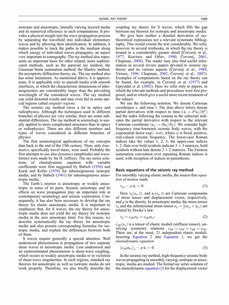
Seismic, Ray Theory, Figure 1 Slowness vector p(perpendicular to the wavefront), ray-velocity vector U (tangentto the ray) and polarization vector g of a P wave propagatingin an isotropic (left) and anisotropic (right) medium. Forsimplicity, the three vectors in the right-hand plot are shown inone plane. In general, this is not the case in anisotropic media.

ing system. Solution of the ray tracing system (25) withappropriate initial conditions yields xiðtÞ, the coordinatesof points along the ray trajectory, and piðtÞ, the Cartesiancomponents of the slowness vectors along the ray. Thetravel time T along the ray is obtained automatically,T ¼ t.

Inserting Equation 21 in Equations 25, we obtain theray tracing system form-th wave in inhomogeneous aniso-tropic media:

dxidt

¼ aijklplgðmÞj gðmÞk ;

dpidt

¼ � 1

2

@ajkln@xi

pkpngðmÞj gðmÞl :

(26)

In the derivation of the first set of Equations 26 for @H =@pi,we took into account that Gik@ðgðmÞi gðmÞk Þ=@pn ¼ 0. Analternative version of ray tracing equation (26) was derivedby Červený (1972), in which the eigenvectors gðmÞ are notused.

The initial conditions for the ray tracing system (26) arexi ¼ x0i, pi ¼ p0i, where x0i and p0i satisfy the eikonalequation (22), corresponding to the wave we wish to com-pute (P, S1 or S2). Components p0i of the initial slownessvector p0 can be then expressed as p0i ¼ n0i=Cðx0iÞ, whereC is the relevant phase velocity. The eikonal equation (22)is then satisfied along the whole ray.

In inhomogeneous isotropic media, the ray tracing sys-tem (25) with Equation 23 yields

dxidt

¼ V 2pi;dpidt

¼ � @lnV@xi

: (27)

The initial conditions for the ray tracing system (27) areagain xi ¼ x0i, pi ¼ p0i, where p0i ¼ n0i=V ðx0iÞ. HereV ¼ a for P waves, and V ¼ b for S waves.

As t is the travel time along the ray, dxi=dt represent theCartesian components U i of the ray-velocity vector U ofthe m-th wave:

U i ¼ aijklplgðmÞj gðmÞk : (28)

In non-dissipative anisotropic media, the ray-velocity

vector U is also called the group-velocity vector orthe energy-velocity vector. As indicated by the name, theenergy velocity vector U represents the velocity ofthe energy propagation.

In anisotropic media, the ray-velocity vectorU must bestrictly distinguished from the phase-velocity vector C. Ininhomogeneous anisotropic media, the ray-velocity andphase-velocity vectors U and C are generally different,both in size and direction. Vector U is always greater thanC. The two vectors are equal (in size and direction) only inspecial directions, called longitudinal directions.

In inhomogeneous isotropic media, Equation 28 for theray-velocity vector yields U ¼ V 2p. For the phase-velocity vector, using Equation 17, we get C ¼ V 2p. Inboth cases, V ¼ a for P waves, and V ¼ b for S waves.Thus, the ray-velocity and phase-velocity vectors are iden-tical in isotropic media.

Figure 1 shows mutual orientation of ray-velocity vec-tor U, phase-velocity vector C (parallel to slownessvector p) and polarization vector g of a P wave propagat-ing in an isotropic (left) and anisotropic (right) medium.WhileU, C and g are parallel in isotropic media, they gen-erally differ in anisotropic media. For S waves, the vectorsU and C have similar orientation as in the case of P waves.The polarization vectors g are, however, perpendicular

SEISMIC, RAY THEORY 1249

(isotropic medium) or nearly perpendicular (anisotropicmedium) to the ray.

Ray tracing systems (26) and (27) can be simply solvedif the initial values x0i and p0i are specified at some point S.We then speak of initial-value ray tracing. The standardnumerical procedures of solving the system of ordinarydifferential equations of the first order with specifiedinitial conditions can then be used (Runge-Kutta,etc.). A very important role in seismology is played byboundary-value ray tracing, in which we seek the ray, sat-isfying some boundary conditions. The typical boundary-value problem is two-point ray tracing, in which we seekthe ray connecting two specified points. Mostly, the con-trolled initial-value ray tracing (controlled shootingmethod) is used to solve this problem (Červený et al.,2007). Boundary-value ray tracing is considerably morecomplicated than initial-value ray tracing.

There are four important differences between initial-value ray tracing in isotropic and anisotropic media. First:In anisotropic media, we deal with three waves, P, S1 andS2, in isotropic media with two waves, P and S, only. Sec-ond: In inhomogeneous anisotropic media, ray tracingsystem (26) is the same for all three waves. The waveunder consideration is specified by the initial conditions,which must satisfy the eikonal equation of the consideredwave. In isotropic inhomogeneous media, the ray tracingsystems are different for P and S waves, see Equations 27with V ¼ a and V ¼ b, respectively. Third: In isotropicmedia, the initial direction of the slowness vector specifiesdirectly the initial direction of the ray (as the tangent to theray and the slowness vector have the same directions). Inanisotropic media, the direction of the ray is, generally,different from the direction of the slowness vector. Never-theless, we have to use p0i as the initial values for the raytracing system. The ray-velocity vector U can be simplycalculated from slowness vector p at any point of theray, including the initial point. Fourth: Ray tracing forP and S waves is regular everywhere in inhomogeneousisotropic media. In anisotropic media, problems arise withtracing S-wave rays in vicinities of singular directions, orif medium is nearly isotropic (quasi-isotropic).

The problem of ray tracing and travel-time computationin inhomogeneous media has been broadly discussed inthe seismological literature; particularly for inhomoge-neous isotropic media. Many ray tracing systems andmany suitable numerical procedures for performing raytracing have been proposed. For 1-D isotropic media (ver-tically inhomogeneous, radially symmetric), the ray trac-ing systems may be simplified so that they reduce tosimple quadratures, well known from classical seismolog-ical textbooks (Aki and Richards, 1980). Standard pro-grams for ray tracing and travel-time computations inlaterally varying isotropic and anisotropic structures areavailable, see, for example, program packages SEIS(2D isotropic models), CRT and ANRAY (3D isotropic/anisotropic models) at http://sw3d.cz/. Programs foranisotropic media have, however, problems with S-wavecomputations in quasi-isotropic media and in the vicinities

of shear-wave singularities. In such cases, the standard raytheory should be replaced by the coupling ray theory.Numerical procedures based on the coupling ray theoryare, unfortunately, rare.

Ray tracing may also serve as a basis for the so-calledwavefront construction method (Gjøystdal et al., 2002). Inthis case, for a selected wave, wavefronts with travel timesT ¼ T0 þ kDT are computed successively from the previ-ous wavefronts with travel times T ¼ T0 þ ðk � 1ÞDT .The wavefront construction method has found broad appli-cations in seismic exploration.

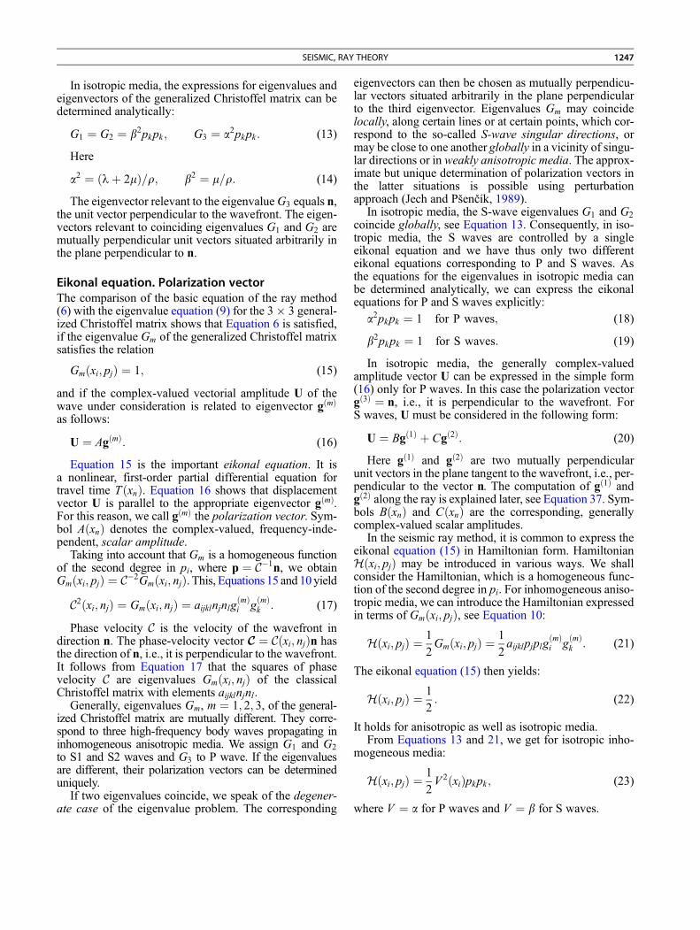
Let us consider a two-parametric system of rays, call itthe ray field, and specify the individual rays in the ray fieldby ray parameters g1; g2. Ray parameters g1; g2 may repre-sent, e.g., the take-off angles at a point source, or the cur-vilinear Gaussian coordinates of initial ray points alongthe initial surface. The family of rays with ray parameterswithin the limit ½g1; g1 þ dg1�, ½g2; g2 þ dg2�, is called theelementary ray tube or briefly the ray tube. We furtherintroduce ray coordinates g1; g2; g3 in such a way thatg1; g2 are ray parameters, and g3 is somemonotonic param-eter along a ray (arclength s, travel time t, etc.). Here weconsider g3 ¼ t, but our results may be simply modifiedfor any other monotonic parameter g3. We further intro-duce the 3� 3 transformation matrix Q from ray to Carte-sian coordinates with elements Qij ¼ @xi=@gj. TheJacobian of transformation from ray to Cartesian coordi-nates, det Q, can be expressed as follows:

det QðtÞ ¼ ð@xðtÞ=@g1 � @xðtÞ=@g2ÞTUðtÞ: (29)

The vectorial product in Equation 29 has the direction

of the normal to the wavefront, specified by n ¼ C p. AspðtÞ UðtÞ ¼ 1, see Equations 28, 10, and 15, we alsoobtain

det QðtÞ ¼ CðtÞjð@xðtÞ=@g1 � @xðtÞ=@g2Þj: (30)

Thus Jacobian det QðtÞ equals CðtÞdOðtÞ, where

dOðtÞ ¼ jð@xðtÞ=@g1 � @xðtÞ=@g2Þj is the scalar surfaceelement cut out of the wavefront by the ray tube. It mea-sures the expansion or contraction of the ray tube, seeFigure 2. For this reason, the 3� 3 matrix QðtÞ is alsooften called the geometrical spreading matrix and variousquantities related to det QðtÞ are called geometricalspreading. It plays an important role in the computationof the ray-theory amplitudes.

Transport equation. Computation of ray-theoryamplitudesThe second equation of the basic system of equations ofthe ray method yields the transport equation for the scalarray-theory amplitude AðxiÞ. The transport equation isa partial differential equation of the first order. It can beexpressed in several forms. One of them, valid both forisotropic and anisotropic media, reads

H ðrA2UÞ ¼ 0: (31)

A0 D0

B0C0

dΩ 0

dΩ

A D

CB

Seismic, Ray Theory, Figure 2 Elementary ray tube. dO0 and dOare scalar surface elements cut out of the wavefront by theray tube. This means that in isotropic media, the normals to dO0and dO are parallel to rays. In anisotropic media, they are not.

1250 SEISMIC, RAY THEORY

It is common to solve the transport equation along the

ray. H U can then be expressed as follows:

H U ¼ d½lnðdet QÞ�=dt (32)

(Červený, 2001, Equation 3.10.24). Inserting Equation 32into Equation 31 yields the transport equation in the formof the first-order ordinary differential equation along theray:

d rðtÞA2ðtÞdet QðtÞ� �=dt ¼ 0: (33)

This yields a simple form of the continuation relation

for AðtÞ along the ray:

AðtÞ ¼ rðt0Þdet Qðt0ÞrðtÞdet QðtÞ

" #1=2Aðt0Þ: (34)

We obtain another suitable continuation relation for

amplitudes along the ray by introducing a special localCartesian coordinate system y1; y2; y3, varying along theray. We call it the wavefront orthonormal coordinate sys-tem. At any point of the ray specified by g3 ¼ t, the y3 axisis parallel to slowness vector p, and the y1; y2 axes are con-fined to the plane tangential to the wavefront at g3 ¼ t.Axes y1 and y2 are mutually perpendicular. If we denotethe 3� 3 transformation matrix from ray coordinates to

wavefront orthonormal coordinates by Qð yÞ

, then

det QðtÞ ¼ det Qð yÞðtÞ ¼ CðtÞdet Qð yÞðtÞ: (35)

Here CðtÞ is the phase velocity, and QðyÞðtÞ is the 2� 2

upper-left submatrix of QðyÞ ðtÞ. Using Equation 35

in Equation 34, we obtain the continuation relation in analternative form:

AðtÞ ¼ rðt0ÞCðt0Þdet Qð yÞðt0ÞrðtÞCðtÞdet Qð yÞðtÞ

" #1=2Aðt0Þ: (36)

An important property of continuation relation (36) is

that det Qð yÞðtÞ is uniquely determined by coordinatesy1 and y2, confined to the plane tangential to the wavefrontat t. Thus, Equation 36 remains valid for any coordinatesystems qi (even nonorthogonal), in which mutuallyperpendicular coordinate axes q1 and q2 are confined tothe plane tangential to the wavefront, but the axis q3 istaken in a different way than y3, for example alongthe ray. This is, e.g., the case of the well-knownray-centered coordinate system q1; q2; q3. We havedet QðqÞðtÞ ¼ det Qð yÞðtÞ.

Transport equations for P and S waves in isotropicmedia may be also expressed in the form of Equation 31.The expression is straightforward for P waves. ForS waves, transport equations for scalar amplitudes B andC in Equation 20 are generally coupled. They decoupleonly if the unit vectors gð1Þ and gð2Þ in Equation 20 satisfythe following relation along the ray:

dgðMÞ=dt ¼ ðgðMÞ HbÞn; M ¼ 1; 2: (37)

In the terminology of the Riemanian geometry, vector gðMÞsatisfying Equation 37 is transported parallelly alongthe ray. If gð1Þ and gð2Þ are chosen as mutually perpendicu-lar and perpendicular to n at one point of the ray, Equa-tion 37 guarantees that they have these properties at anypoint of the ray. Consequently, gð1Þ and gð2Þ are always per-pendicular to the ray and do not rotate around it as theSwave progresses. As gð1Þ, gð2Þ and n are always orthonor-mal, and n is known at any point of the ray, it is not neces-sary to use Equation 37 to compute both vectors gðMÞ. Oneof them can be determined from the orthonormality condi-tion, once the other has been computed using Equation 37.

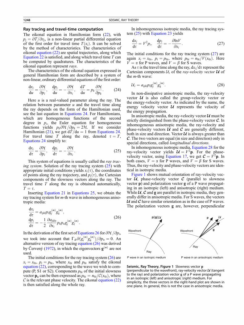
Quantity det QðtÞ in Equation 34 may be zero at somepoint t ¼ tC . This means that the cross-sectional area ofthe ray tube shrinks to zero at t ¼ tC . The relevant pointt ¼ tC of the ray is called the caustic point. At the causticpoint, the ray solution is singular and yields an infiniteamplitude there. In passing through the caustic point tCalong the ray, the argument of ½det QðtÞ�1=2 may changeby p=2 or p (Kravtsov and Orlov, 1999). The formercase corresponds to the caustic point of the first order, seeFigure 3a, during which the ray tube shrinks to an elemen-tary arc, the latter case corresponds to the caustic point ofthe second order, see Figure 3b, during which the ray tubeshrinks to a point. It is common to introduce the phaseshift due to caustic TCðt; t0Þ using the relation

det Qðt0Þdet QðtÞ

" #1=2¼ det Qðt0Þ

det QðtÞ

����������1=2

exp½iTCðt; t0Þ� (38)

if caustic point tC is situated between t0 and t. The phaseshift due to the caustic is cumulative. If the ray passesthrough several caustic points along the ray between t0and t, the phase shift due to caustics is the sum of theindividual phase shifts. It is often expressed in the formTCðt; t0Þ ¼ �1

2pkðt; t0Þ, where kðt; t0Þ is an integer,

A0 B0

C0D0

AB

CD

AB

C D

A0 B0

C0D0

a

b

Seismic, Ray Theory, Figure 3 Caustic points of (a) the first order and (b) second order. (Figure 3.13 of Cerveny, 2001.)

SEISMIC, RAY THEORY 1251

called the KMAH index (to acknowledge the work by -Keller, Maslov, Arnold and Hörmander in this field).The continuation relation for ray-theory amplitudes (34)can then be modified to read:

AðtÞ ¼ rðt0Þjdet Qðt0ÞjrðtÞjdet QðtÞj

!1=2

exp½iTCðt; t0Þ�Aðt0Þ:

(39)

Equation 36 can be transformed to the analogous form asEquation 39 as the zeros of det QðyÞðtÞ are situated at thesame points tC on the ray as the zeros of det QðtÞ.

The KMAH index can be calculated along the ray asa byproduct of dynamic ray tracing. For detailed deriva-tions and discussion see Bakker (1998) and Klimeš(2010).

There are some differences between the KMAH indicesalong the rays in isotropic and anisotropic media. In iso-tropic media, the KMAH index always increases whenthe ray passes through a new caustic point, either by oneor two. In anisotropic media, however, it may alsodecrease by one or two at some caustic points. This hap-pens only for S waves as a consequence of the concaveform of the slowness surface of the corresponding S wave.

Dynamic ray tracing. Paraxial approximationsAs we can see in Equation 34, the computation of the ray-theory amplitudes requires knowledge of det Q, whereQðtÞ characterizes the properties of the ray field in thevicinity of the ray under consideration. QðtÞ can be com-puted by the procedure called dynamic (or paraxial) raytracing. In addition to QðtÞ with elements

QijðtÞ ¼ @xi=@gj, we also have to introduce a new 3� 3matrix PðtÞ with elements PijðtÞ ¼ @pi=@gj. The equationfor Pij must be included to obtain the linear dynamic raytracing system. Differentiating ray tracing equations (25)with respect to gj, we can easily obtain a system of linearordinary differential equations of the first order for Qijand Pij,

dQij

dt¼ @2H

@pi@xkQkj þ @2H

@pi@pkPkj;

2 2

dPij

dt¼ � @ H

@xi@xkQkj � @ H

@xi@pkPkj; (40)

see Červený (1972). This system is usually called thedynamic ray tracing system, and the relevant proceduredynamic ray tracing. It can be solved along a given rayO, or together with it.

The dynamic ray tracing system (40) may be expressedin various forms. Instead of Cartesian coordinates xi, wecan use the wavefront orthonormal coordinates yi, or theray-centered coordinates qi. Then, instead of the 3� 3matrices Q and P, it is sufficient to seek the 2� 2 matricesQðyÞ, PðyÞ or QðqÞ, PðqÞ. This reduces the number of DRTequations, but complicates their right-hand sides (Červený2001, sect. 4.2).

As the dynamic ray tracing system (40) is of the firstorder and linear, we can compute its fundamental matrixconsisting of six linearly independent solutions. The6� 6 fundamental matrix of system (40) specified bythe 6� 6 identity matrix at an arbitrary point t ¼ t0 ofthe ray is called the ray propagator matrix and denotedby Pðt; t0Þ.

Ray ΩRay Ω

1252 SEISMIC, RAY THEORY

The 6� 6 ray propagator matrixPðt; t0Þ is symplectic:

PT t; t0Þð JP t; t0Þð ¼ J; with J ¼ 0 I�I 0

� �(41)

If we know the matrices Qðt Þ, Pðt Þ, we can compute

Plane-wavefrontinitial conditions

Point-sourceinitial conditions

τ0

τ0

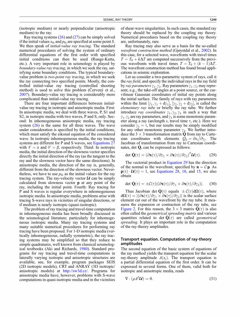
Seismic, Ray Theory, Figure 4 Plane-wavefront and point-source initial conditions for dynamic ray tracing. In anisotropicmedia, rays are not perpendicular to the wavefront.

0 0QðtÞ, PðtÞ at any point t of the ray by a simple matrixmultiplication

QðtÞPðtÞ

� �¼ Pðt; t0Þ Qðt0Þ

Pðt0Þ� �

: (42)

The ray propagator matrixPðt; t0Þ satisfies the chain rule,Pðt; t0Þ ¼ Pðt; t1ÞPðt1; t0Þ, where point t1 is situatedarbitrarily on the ray. It is simple to compute the inverseof Pðt; t0Þ: P�1ðt; t0Þ ¼ Pðt0; tÞ. We can expressPðt; t0Þ in the following way:

Pðt; t0Þ ¼ Q1 ðt; t0Þ Q2 ðt; t0ÞP1 ðt; t0Þ P2 ðt; t0Þ

� �; (43)

where Q1 ðt; t0Þ; Q2 ðt; t0Þ; P1 ðt; t0Þ and P2 ðt; t0Þ are3� 3 matrices.

Equation 42 can be used to obtain a very importantquantity – the 3� 3 matrix MðtÞ of second derivativesof the travel-time field with respect to Cartesian coordi-nates, with elements Mij ¼ @2T=@xi@xj:

MðtÞ ¼ PðtÞðQðtÞÞ�1: (44)

Matrix MðtÞ plays an important role in the computation

of travel time not only along the rayO, but also in its “qua-dratic” paraxial vicinity:

TðxÞ ¼ TðxOÞ þ ðx� xOÞTpðtÞþ 12ðx� xOÞTMðtÞðx� xOÞ:

(45)

In Equation 45, x denotes an arbitrary point in the

paraxial vicinity of the ray O, close to point xO ¼ xOðtÞon the ray O; slowness vector pðtÞ and the matrix MðtÞare given at xO. The possibility of computing the traveltime in the paraxial vicinity of the ray has many importantapplications.

The properties of the 6� 6 ray propagator matrixPðt; t0Þ described above remain valid even for the 4� 4ray propagator matrices PðyÞðt; t0Þ or PðqÞðt; t0Þexpressed in wavefront orthonormal coordinates yi orray-centered coordinates qi. The ray propagator matricesPðyÞðt; t0Þ and PðqÞðt; t0Þ are identical, therefore, theycan be expressed in terms of the same 2� 2 matricesQ1ðt; t0Þ, Q2ðt; t0Þ, P1ðt; t0Þ and P2ðt; t0Þ. MatricesQ1ðt; t0Þ, P1ðt; t0Þ correspond to the plane-wavefront ini-tial conditions at t0, and matrices Q2ðt; t0Þ, P2ðt; t0Þ tothe point-source initial conditions at t0, see Figure 4.The 2� 2 matrix Q2ðt; t0Þ plays an important role incomputing the ray-theory Green function. The quantity

Lðt; t0Þ ¼ jdet Q2ðt; t0Þj1=2 (46)

is called the relative geometrical spreading. It correspondsto a point source.

As in Equation 44, we can define the 2� 2 matrix ofthe second derivatives of the travel-time field with respectto y1, y2 or q1, q2 as follows:

MðtÞ ¼ PðtÞðQðtÞÞ�1: (47)

We will now briefly summarize several useful ray-

theory quantities and applications, which rely fully orpartly on dynamic ray tracing. For derivations and moredetailed explanations, seeČervený (2001, Chap. 4), wherealso many other applications and references can be found:(1) Paraxial travel times. (2) Paraxial slowness vectors.(3) Paraxial rays. (4) Curvature of the wavefront.(5) Matrix of geometrical spreading Q and the relevantmatrix P. (6) Continuation relations for ray-theory ampli-tudes along the ray. (7) Relative geometrical spreading.(8) Phase shift due to caustics. (9) Ray-theoryelastodynamic Green function. (10) Higher-order spatialderivatives of the travel-time field. (11) Fresnel volumesand Fresnel zones. (12) Surface-to-surface propagatormatrix. (13) Boundary-value problems in four-parametricsystem of paraxial rays, including two-point ray tracing.(14) Factorization of the geometrical spreading.

Dynamic ray tracing is also needed in the investigationof ray chaos and in computations of Lyapunov exponents,in the ray-perturbation methods and in modifications andextensions of the ray method such as Maslov method,Gaussian beam and Gaussian packet summation methods,in Kirchhoff-Helmholtz method and in various diffractionmethods.

Coupling ray theory for S waves in anisotropicmediaIn inhomogeneous weakly anisotropic media, the standardray theory described above yields distorted results since itis unable to describe the coupling of S1 and S2 wavespropagating with approximately equal phase velocities.This problem can be removed by using the coupling ray

SEISMIC, RAY THEORY 1253

theory. In the coupling ray theory, the amplitudes of thetwo S waves can be computed along a trajectory calledthe common ray (Bakker, 2002; Klimeš, 2006). The closerthe common ray approximates actual S-wave rays, themore accurate results the coupling ray theory yields. Thecommon rays can be constructed in a reference isotropicmedium or in the actual anisotropic medium.A convenient option is to compute common rays usingray tracing equations (25) with the Hamiltonian given as

Hðxi; pjÞ ¼ 14½G1ðxi; pjÞ þ G2ðxi; pjÞ�: (48)

In Equation 48, G and G are eigenvalues of the

1 2Christoffel matrix G, see equation (7), corresponding toS1 and S2 waves.

The coupling ray theory solution is sought in the form(Coates and Chapman, 1990; Bulant and Klimeš, 2002):

uðt; tÞ ¼ AðtÞ½r1ðtÞgð1ÞðtÞexpðiot1Þþ r2ðtÞgð2ÞðtÞexpðiot2Þ�expð�iotÞ:

(49)

Here, AðtÞ is the scalar amplitude (34) or (36) calculatedalong the common ray. The symbols gð1Þ and gð2Þ denotethe S-wave eigenvectors of the generalized Christoffelmatrix Gðxi; pjÞ calculated along the common ray. Thetravel times t1 and t2 are travel times corresponding tothe above vectors gð1Þ and gð2Þ. They can be obtained byquadratures along the common ray:

dt1=dt ¼ ½Gikgð1Þi gð1Þk ��1=2;

dt2=dt ¼ ½Gikgð2Þi gð2Þk ��1=2:

(50)

The amplitude factors r1 and r2 are solutions of twocoupled ordinary differential equations (Coates andChapman, 1990):

dr1=dt

dr2=dt

� �¼ dj

dt0 expðio½t2ðtÞ�t1ðtÞ�Þ

�expðio½t1ðtÞ�t2ðtÞ�Þ 0

� �r1r2

� �;

(51)

where the angular velocity dj=dt of the rotation of theeigenvectors gð1Þ and gð2Þ is given by

djdt

¼ gð2Þdgð1Þ

dt¼ �gð1Þ

dgð2Þ

dt: (52)

For detailed description of the algorithm, see Bulant andKlimeš (2002).

There are many possible modifications and approxima-tions of the coupling ray theory. In some of them, theamplitude vector U of coupled S waves is sought alongthe common ray in the form of Equation 20, in which theamplitude factors B and C can be expressed as

BðtÞ ¼ AðtÞBðtÞ CðtÞ ¼ AðtÞCðtÞ: (53)

In Equations 53, AðtÞ is again the scalar ray amplitude, seeequation (34) or (36), calculated along the commonS-wave ray. There are many ways how to evaluate factorsB and C (Kravtsov, 1968; Pšenčík, 1998; Červený et al.,2007). Here we present a combination of coupling ray the-ory and of the first-order ray tracing (Farra and Pšenčík,2010). In the approximation of Farra and Pšenčík (2010),the common ray is obtained as the first-order ray, see sec-tion on ray perturbation methods. The vectors gðKÞ,appearing in Equation 20, specify the first-order approxi-mation of the S-wave polarization plane. The factors Band C in Equations 53 are then obtained as a solution oftwo coupled ordinary differential equations, which resultfrom the corresponding two coupled transport equations:

dB=dtdC=dt

� �¼ � io

2

M11 � 1 M12

M12 M22 � 1

� � BC

� �:

(54)

Evaluation of the matrixMwith elementsM is sim-

IJple (see Farra and Pšenčík (2010); Equations 20 and 7).

The resulting equations reduce to standard ray-theoryequations in inhomogeneous isotropic media, theydescribe properly S-wave coupling in inhomogeneousweakly anisotropic media and even yield separateS waves when anisotropy is stronger. Common S-waverays are regular everywhere. They do not suffer from prob-lems well known from tracing rays of individual S wavesin anisotropic media and are suitable for investigatingshear-wave splitting.

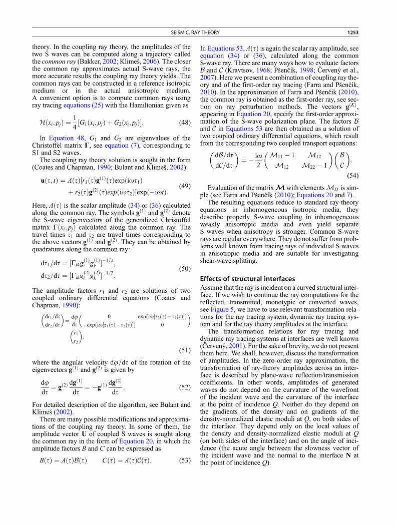
Effects of structural interfacesAssume that the ray is incident on a curved structural inter-face. If we wish to continue the ray computations for thereflected, transmitted, monotypic or converted waves,see Figure 5, we have to use relevant transformation rela-tions for the ray tracing system, dynamic ray tracing sys-tem and for the ray theory amplitudes at the interface.

The transformation relations for ray tracing anddynamic ray tracing systems at interfaces are well known(Červený, 2001). For the sake of brevity, we do not presentthem here. We shall, however, discuss the transformationof amplitudes. In the zero-order ray approximation, thetransformation of ray-theory amplitudes across an inter-face is described by plane-wave reflection/transmissioncoefficients. In other words, amplitudes of generatedwaves do not depend on the curvature of the wavefrontof the incident wave and the curvature of the interfaceat the point of incidence Q. Neither do they depend onthe gradients of the density and on gradients of thedensity-normalized elastic moduli at Q, on both sides ofthe interface. They depend only on the local values ofthe density and density-normalized elastic moduli at Q(on both sides of the interface) and on the angle of inci-dence (the acute angle between the slowness vector ofthe incident wave and the normal to the interface N atthe point of incidence Q).

Interface Σ

S2S1

P

P

S1S2

NIncidentwave

Seismic, Ray Theory, Figure 5 Slowness vectors of P, S1 and S2waves generated at the point of incidence Q of a curvedinterface separating two inhomogeneous anisotropic media. Allslowness vectors at Q are situated in the plane of incidencespecified by the slowness vector of the incident wave and thenormal to the interface N at Q. Ray-velocity vectors (tangent torays) of individual waves atQ are, in general, not confined to theplane of incidence. In isotropic media, instead of reflected andtransmitted S1 and S2 waves, single reflected and transmittedS waves are generated. In inhomogeneous weakly anisotropicmedia, single coupled S waves are generated. Ray-velocityvectors of individual waves at Q are situated in the plane ofincidence in isotropic media.

1254 SEISMIC, RAY THEORY

Various types of R/T coefficients may be used. The dis-placement R/T coefficients are used most frequently (Akiand Richards, 1980; Červený et al., 1977 for isotropicmedia; Fedorov, 1968 for anisotropic media). Very usefulare the energy R/T coefficients, as they are reciprocal. Therelation between the energy R/T coefficientRðQÞ and thedisplacement R/T coefficient RðQÞ is as follows:

RðQÞ ¼ RðQÞ rð~QÞUnð~QÞrðQÞUnðQÞ 1=2

(55)

(Červený 2001, sect. 5.4.3). Here Q is the point of

incidence, and ~Q the relevant initial point of the R/Twave, both points being, of course, identical. Un is thenormal component (perpendicular to the interface) ofthe ray-velocity vector. We further introduce the completeenergy R/TcoefficientsRC along the ray using the relation

RC ¼YNk¼1

RðQkÞ: (56)

The complete energy R/T coefficient RC corresponds tothe ray which interacts N -times with interfaces (at pointsof incidence Q1;Q2; :::;QN ) between the initial and endpoint of the ray.

Generalization of the continuation relation (36) for theray-theory amplitudes along the ray situated in a laterallyvarying anisotropic medium containing curved interfacesthen reads:

AðtÞ ¼ rðt0ÞCðt0Þjdet QðyÞðt0ÞjrðtÞCðtÞjdet QðyÞðtÞj

!1=2

RCexp½iTCðt; t0Þ�Aðt0Þ:(57)

In seismic prospecting, in the technique called ampli-

tude variation with offset (AVO), it is common to workwith the so-called weak-contrast R/T coefficients. Theyare linearized versions of exact R/T displacement coeffi-cients. Linearization is mostly made with respect to thecontrasts of the density and elastic moduli across the inter-face. There is a great variety of linearized formulaedepending on the type of media surrounding the interface(isotropic, anisotropic), strength of anisotropy (weak,strong), etc. The coefficients yield reasonable approxima-tion in the vicinity of normal incidence. For increasingincidence angles, their accuracy decreases. The advantageof the weak-contrast coefficients is their simplicity and thepossibility of expressing them in explicit form. The effectsof the individual medium parameters on the coefficientscan than be easily evaluated.

Ray-theory elastodynamic Green functionThe elastodynamic Green function GinðR; t; S; t0Þ repre-sents the i-th Cartesian component of the displacementvector at location R and time t, due to a single-force pointsource situated at location S and oriented along the n-thCartesian axis, with the time dependence dðt � t0Þ. Weintroduce quite analogously the ray-theory elastodynamicGreen function, with only two differences. The first differ-ence is that ray-theory Green function is defined as a sumof elementary ray-theory Green functions computed alongrays of selected elementary waves (direct, multiplyreflected/transmitted, etc.). The second difference is thatthe elementary ray-theory Green functions are not exact,but only zero-order ray approximations.

In the frequency domain the elementary ray-theoryelastodynamic Green function GinðR; S;oÞ for t0 ¼ 0reads:

GinðR; S;oÞ ¼ gnðSÞgiðRÞexp½iTGðR; SÞ þ ioTðR; SÞ�4p½rðSÞrðRÞCðSÞCðRÞ�1=2LðR; SÞ

RC:

(58)

Here LðR; SÞ is the relative geometrical spreading,given by Equation 46, giðRÞ and gnðSÞ are the eigenvec-tors of the generalized Christoffel matrix at R and S (polar-ization vectors corresponding to the consideredelementary wave), T is the travel time along theray from S to R, RC the complete energy R/T coefficientresulting from interactions of the ray under considerationwith interfaces between S and R, and TGðR; SÞ the com-plete phase shift due to caustics along the ray between Sand R. The relevant KMAH index in anisotropic mediamay also include a contribution at a point source S (ifthe slowness surface of the considered wave is concaveat S). In isotropic media, this contribution is always zero.

The complete energy R/T coefficient RC , the traveltime TðR; SÞ, the relative geometrical spreading LðR; SÞand the complete phase shift due to caustics are alwaysreciprocal. Consequently, the elementary ray-theory

SEISMIC, RAY THEORY 1255

elastodynamic Green function satisfies a very importantproperty of reciprocity:

GinðR; S;oÞ ¼ GniðS;R;oÞ: (59)

This relation is valid for any elementary seismic bodywave generated by a point source.

For elementary ray-theory Green functions in inhomo-geneous weakly anisotropic media see Pšenčík (1998).

Chaotic rays. Lyapunov exponentsIn homogeneous media, geometrical spreading increaseslinearly with increasing length of the ray. In heterogeneousmedia, behavior of geometrical spreading is more compli-cated, and depends considerably on the degree of hetero-geneity of the medium. In models, in which theheterogeneity exceeds certain degree, average geometricalspreading increases exponentially with increasing lengthof the ray. Rays in such a medium often exhibit chaoticbehavior, which is characterized by a strong sensitivityof rays to the initial ray data (for example, to ray parame-ters). The rays with only slightly differing ray data at aninitial point tend to diverge exponentially at large dis-tances from the initial point. Consequently, the rays inter-sect many times and many rays pass through the samepoint. With such chaotic rays, two-point ray tracing ispractically impossible, and the ray tubes are not narrowenough for travel time interpolation. The chaotic behaviorof rays increases with increasing length of rays and pre-vents applicability of the ray theory.

The exponential divergence of chaotic rays in the phasespace (the space formed by spatial coordinates xi andslowness-vector components pj) can be quantified by theso-called Lyapunov exponents. They may be introducedin several ways. It is common to express them in termsof characteristic values of the ray propagator matrix.The relevant expressions for the Lyapunov exponentsand several numerical examples for 2D models withoutinterfaces can be found in Klimeš (2002a). See alsoČervený et al. (2007), where other references can befound.

The estimate of the Lyapunov exponent of a singlefinite ray depends on its position and direction. TheLyapunov exponents associated with rays of differentpositions and directions can be used to calculate averageLyapunov exponents for the model. The averageLyapunov exponents play a very important role in smooth-ing the models so that they are suitable for ray tracing(Červený et al., 2007).

Ray perturbation methodsRay perturbation methods represent an important part ofthe ray theory. They can be used for approximate but fastand transparent solutions of forward problems in compli-cated models. They play even more important role in theinverse problems.

Ray perturbation methods are useful everywhere,where we wish to compute the wavefield or its

constituents (travel times, amplitudes, polarization) incomplicated models, which deviate only little from sim-ple, reference models, for which computations are simpler.The solutions for complicated models are then sought asperturbations of simpler solutions for the referencemodels. Examples are computations in weakly anisotropicmedia, which use an isotropic medium as reference, or inweakly dissipative media, which use a perfectly elasticmedium as reference. Basic role in these approaches isplayed by reference rays traced in reference media. Solu-tions in perturbed media can be given in the form ofa power series in the deviations of the perturbed and refer-ence models. Mostly, the first-order approximation, i.e.the first term of the power series, is used.

The most frequent application of ray perturbationmethods is in travel-time computations. First-ordertravel-time perturbation formulae for isotropic media areknown and have been used (mostly in tomography) forseveral decades. Well known and broadly applied are alsofirst-order travel-time formulae for anisotropic media(Červený and Jech, 1982; Hanyga, 1982; Červený, 2001,sect. 3.9). Travel-time perturbations are obtained by quad-ratures along reference rays. As integration parameters,the parameters along reference rays are used.

Recently, several procedures for computation of higher-order travel-time perturbations for weakly anisotropicmedia (note that anisotropy of the Earth is mostly weak)were proposed. The procedure based on the so-called per-turbation Hamiltonians (Klimeš, 2002b; Červený et al.,2007) allows computation of highly accurate travel timesalong a fixed reference ray in a reference medium.Another procedure is based on the so-called first-orderray tracing described briefly below. In the latter method,second-order travel-time perturbations can be calculatedalong first-order rays.

Relatively recent is the use of ray perturbation methodsin first-order ray tracing and first-order dynamic ray trac-ing (Pšenčík and Farra, 2007; Farra and Pšenčík, 2010). Itallows to compute, approximately, not only rays and traveltimes, but whole wavefields. To derive first-order ray trac-ing and dynamic ray tracing, the perturbation approach isused in which deviations of anisotropy from isotropy areconsidered to be of the first order. Then it is just sufficientto use Equations 25 and 40 with Equation 21, in which theexact eigenvalue Gm is replaced by its first-order approxi-mation. The resulting ray tracing provides first-order rays,first-order travel times and the first-order geometricalspreading. By simple quadratures along first-order rays,second-order travel-time corrections can be computed.This approach is applicable to P and S waves. In case ofS waves, it can include the computation of couplingeffects. First-order ray tracing and dynamic ray tracingare used in this case for computing common rays, first-order travel times and geometrical spreading along them,using the Hamiltonian (48). The wavefield of S waves isobtained by solving second-order coupling equationsalong the common rays. The procedure yields standardray-theory results for S waves propagating in isotropic

1256 SEISMIC, RAY THEORY

media, and approximate results in anisotropic media whenthe S waves are coupled or even decoupled.

Ray perturbation method for weakly dissipativemediaIn viscoelastic media, the density-normalized stiffnesstensor aijkl is complex valued:

aijklðxnÞ ¼ aRijklðxnÞ � iaIijklðxnÞ: (60)

If aI is small, the viscoelastic medium can be consid-

ijklered as a perturbation of a perfectly elastic medium(Červený, 2001, sect. 5.5.3) which has a form of the imag-inary-valued term � iaIijkl. Reference ray in the referenceperfectly elastic medium and corresponding real-valuedtravel time T along the reference ray between pointsS and R can be obtained by standard ray tracing in per-fectly elastic media. The imaginary travel time TI

(travel-time perturbation due to � iaIijkl) can be thenobtained by quadratures along the reference ray:

TI ¼ 12

Z R

SQ�1ðtÞdt: (61)

The quantity Q in Equation 61 is a direction-dependentquality factor for anisotropic media, corresponding tothe Hamiltonian (21):

Q�1 ¼ aIijklpjplgigk : (62)

For general Hamiltonians, the quality factor Q is givenby the relation Q�1 ¼ �ImHðxi; pjÞ.

The imaginary travel time TI in Equation 61 is respon-sible for the exponential amplitude decay along the refer-ence ray. For causal dissipation, the stiffness tensor (60)is frequency dependent. The above described perturbationapproach is then equivalent to the perturbation scheme, inwhich aIijklðxn;oÞ is considered to be of the order of o�1

for o ! ? (Kravtsov and Orlov, 1990; Gajewski andPšenčík, 1992).

In an inhomogeneous isotropic, weakly dissipativemedium, the expression (62) reduces to the well-knownformula

Q�1 ¼ �ImV 2=ReV 2¼: � 2ImV=ReV ; (63)

in which V is the complex-valued velocity, V ¼ a forP waves and V ¼ b for S waves. Complex-valued quanti-ties a and b are generalizations (to the complex space) ofreal-valued a and b from Equation 14.

Concluding remarks. Applications, modifications,and extensions of the ray methodSeismic ray method has found broad applications both inglobal seismology and in seismic exploration. The advan-tages of the seismic ray method consist in its numericalefficiency, universality, conceptual clarity, and in its abil-ity to investigate various seismic body waves

independently of other waves. Although its accuracy isonly limited, the seismic ray method is the only methodwhich is able to give an approximate answer to manyproblems of high-frequency seismic body wave propaga-tion in laterally varying, isotropic or anisotropic, perfectlyelastic or dissipative, layered and block structures.

In classical global seismology, the seismic ray methodhas been traditionally used to study the internal structureof the whole Earth, assuming that the Earth is radiallysymmetric. The standard Earth’s model, obtained in thisway, is expressed in terms of distribution of elastic veloc-ities as a function of depth.

At present, the applications of the seismic raymethod areconsiderably broader. It is broadly used to study the 3-Dlocal lateral inhomogeneities in the structure, the form andphysical properties of structural interfaces, the local anisot-ropy, attenuation, etc. In addition to forward modeling, theray perturbation methods are also broadly used for inver-sions based on measured travel times or whole waveforms.In lithospheric structural studies, particularly in crustal seis-mology, the ray-synthetic seismograms have been alsooften used for ultimate comparison with observedseismograms. The computation of ray-syntheticseismograms requires determination of not only traveltimes, but also ray-theory amplitudes and polarization ofindividual waves. Seismic ray method has also found broadapplications in other branches of seismology. Very impor-tant examples are the localization of seismic sources andthe simultaneous localization with structural inversion.

In most applications of the raymethod in seismic explo-ration for oil, the use of local 3-D structures with structuralcurved interfaces is a necessity. Sophisticated algorithmshave been developed and used to image the structuresunder consideration. At present, the most important roleis played by migration algorithms. Seismic ray theoryand its extensions have found important applications inthese algorithms.

The raymethod is not valid universally.We have brieflydescribed three serious limitations of the ray method:(a) The ray method can be used only for high-frequencysignals. (b) In models, in which heterogeneity of themedium exceeds certain degree, the ray field has chaoticcharacter, particularly at large distances from the source.(c) The standard ray method cannot be used for computingS waves propagating in inhomogeneous, weakly aniso-tropic media. It must be replaced by the coupling ray the-ory. The coupling ray theory must be used even inmoderately or strongly anisotropic media, in the vicinityof shear-wave singular directions.

The ray method fails, however, even in other singularsituations. In smooth isotropic media, the most importanttype of singularity are caustics. Caustics may attain vari-ous forms. Various extensions of the ray method can beused to compute wavefields in caustic regions. Theseextensions are frequency dependent. See a detailed treat-ment of wavefields in caustic regions in Kravtsov andOrlov (1999), and also in Stamnes (1986). In models with

SEISMIC, RAY THEORY 1257

smooth structural interfaces, other singularities oftenappear. For edge and vertex points, see Ayzenberg et al.(2007). For critical singular regions, at which head wavesseparate from reflected waves, see Červený and Ravindra(1971). For the waves, whose rays are tangential to inter-faces, see Thomson (1989).

Specific methods, designed for different types of singu-larities may be used for computing wavefields in singularregions. Disadvantage of these methods is that they aredifferent for different singularities. Morever, singularregions often overlap, and the wavefield in the overlapingregion requires again different treatment. It is desirable tohave available a more general extension of the raymethod,applicable uniformly in any of the mentioned singularregions, or, at least, in most of them. Such an extensionwould simplify ray computations considerably and couldeven lead to more accurate results.

Several such extensions of the ray method have beenproposed. We do not describe them here in detail. Instead,we merely present references, in which more details andfurther references can be found. Let us mention theMaslov asymptotic ray theory introduced to seismologyby Chapman and Drummond (1982), see also Thomsonand Chapman (1985), Chapman (2004). Another exten-sion of the ray method is based on the summation ofGaussian beams (Popov, 1982; Červený et al., 1982).For the relation of this method with the Maslov methodsee Klimeš (1984). The Gaussian beam summationmethod has found applications both in the forward model-ing of seismic wavefields and in migrations in seismicexploration. It is closely related to the method of summa-tion of Gaussian packets (Červený et al., 2007). Ray the-ory can be also used in the Born scattering theory(Chapman and Coates, 1994; Chapman, 2004). For wavesreflected from a smooth structural interface separating twoheterogeneous, isotropic or anisotropic media, the Kirch-hoff surface integral method can be used. For details andmany references see Chapman (2004, sect. 10.4). Anotheruseful extension of the ray method is the one-way waveequation approach (Thomson, 1999).

Acknowledgments

The authors are very grateful to Luděk Klimeš and RaviKumar for valuable comments and recommendations.The research was supported by the consortium projectSeismic Waves in Complex 3-D Structures, by researchprojects 205/07/0032 and 205/08/0332 of the GrantAgency of the Czech Republic; and by research projectMSM0021620860 of the Ministry of Education of theCzech Republic.

BibliographyAki, K., and Richards, P., 1980. Quantitative Seismology. San

Francisco: WH Freeman.Ayzenberg, M. A., Aizenberg, A. M., Helle, H. B., Klem-Musatov,

K. D., Pajchel, J., and Ursin, B., 2007. 3D diffraction modeling

of singly scattered acoustic wavefields based on the combinationof surface integral propagators and transmission operators. Geo-physics, 72, SM19–SM34.

Babich, V.M., 1956. Raymethod of the computation of the intensityof wave fronts (in Russian). Doklady Akademii Nauk SSSR, 110,355–357.

Babich, V. M., 1961. Ray method of the computation of theintensity of wave fronts in elastic inhomogeneous anisotropicmedium. In Petrashen, G. I. (ed.), Problems of the DynamicTheory of Propagation of Seismic Waves 77 (in Russian). Lenin-grad: Leningrad University Press, Vol. 5, pp. 36–46. Translationto English: Geophysical Journal International., 118: 379–383,1994.

Bakker, P. M., 1998. Phase shift at caustics along rays inanisotropic media. Geophysical Journal International, 134,515–518.

Bakker, P. M., 2002. Coupled anisotropic shear-wave ray tracing insituations where associated slowness sheets are almost tangent.Pure and Applied Geophysics, 159, 1403–1417.

Bulant, P., and Klimeš, L., 2002. Numerical algorithm of the cou-pling ray theory in weakly anisotropic media. Pure and AppliedGeophysics, 159, 1419–1435.

Červený, V., 1972. Seismic rays and ray intensities in inhomoge-neous anisotropic media. Geophysical Journal of Royal Astro-nomical Society, 29, 1–13.

Červený, V., 2001. Seismic Ray Theory. Cambridge: CambridgeUniversity Press.

Červený, V., and Jech, J., 1982. Linearized solutions of kinematicproblems of seismic body waves in inhomogeneous slightlyanisotropic media. Journal of Geophysics, 51, 96–104.

Červený, V., and Ravindra, R., 1971. Theory of Seismic HeadWaves. Toronto: Toronto University Press.

Červený, V., Molotkov, I. A., and Pšenčík, I., 1977. Ray Method inSeismology. Praha: Univerzita Karlova.

Červený, V., Popov, M. M., and Pšenčík, I., 1982. Computation ofwave fields in inhomogeneous media. Gaussian beam approach.Geophysical Journal of Royal Astronomical Society, 70,109–128.

Červený, V., Klimeš, L., and Pšenčík, I., 1988. Complete seismicray tracing in three-dimensional structures. In Doornbos, D. J.(ed.), Seismological Algorithms. New York: Academic, pp.89–168.

Červený, V., Klimeš, L., and Pšenčík, I., 2007. Seismic ray method:recent developments.Advances in Geophysics, 48, 1–126. http://www.sciencedirect.com/science/bookseries/00652687.

Chapman, C. H., 2002. Seismic ray theory and finite frequencyextensions. In Lee, W. H. K., Kanamori, H., and Jennings,P. C. (eds.), International Handbook of Earthquake andEngineering Seismology, Part A. New York: Academic, pp.103–123.

Chapman, C. H., 2004. Fundamentals of Seismic Wave Propaga-tion. Cambridge: Cambridge University Press.

Chapman, C. H., and Coates, R. T., 1994. Generalized Born scatter-ing in anisotropic media. Wave Motion, 19, 309–341.

Chapman, C. H., and Drummond, R., 1982. Body-waveseismograms in inhomogeneous media usingMaslov asymptotictheory. Bulletin of the Seismological Society of America, 72,S277–S317.

Coates, R. T., and Chapman, C. H., 1990. Quasi–shear wave cou-pling in weakly anisotropic 3-D media. Geophysical JournalInternational, 103, 301–320.

Farra, V., and Pšenčík, I., 2010. Coupled Swaves in inhomogeneousweakly anisotropic media using first-order ray tracing.Geophys-ical Journal International, 180, 405–417.

Fedorov, F. I., 1968. Theory of Elastic Waves in Crystals. NewYork:Plenum.

Free surface

Station

Interface

SP

Earthquake

P wave

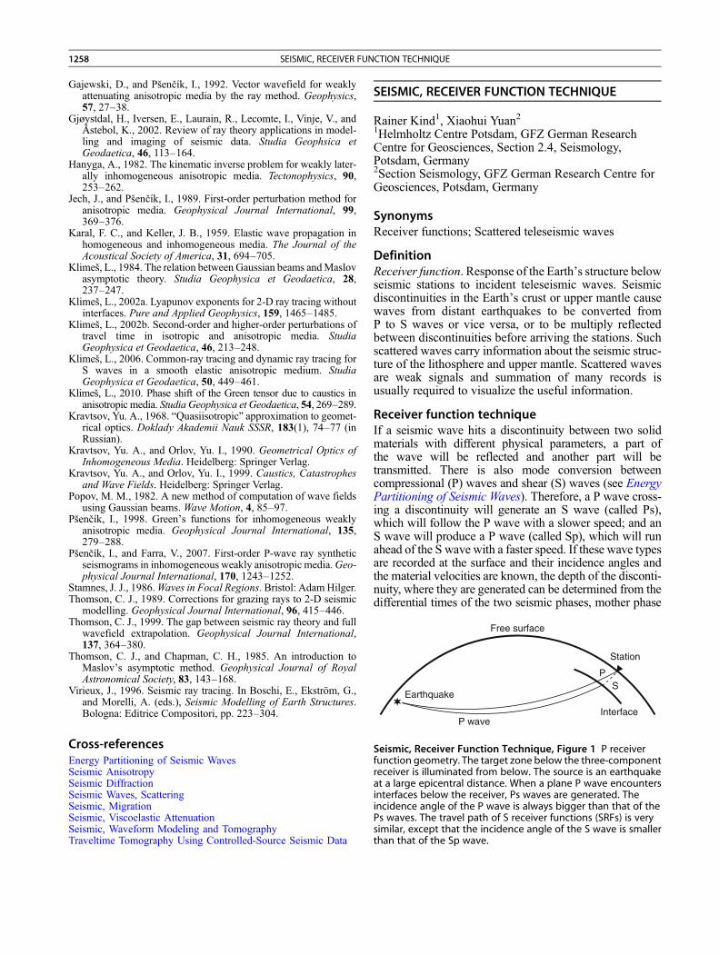
Seismic, Receiver Function Technique, Figure 1 P receiverfunction geometry. The target zone below the three-componentreceiver is illuminated from below. The source is an earthquakeat a large epicentral distance. When a plane P wave encountersinterfaces below the receiver, Ps waves are generated. Theincidence angle of the P wave is always bigger than that of thePs waves. The travel path of S receiver functions (SRFs) is verysimilar, except that the incidence angle of the S wave is smallerthan that of the Sp wave.

1258 SEISMIC, RECEIVER FUNCTION TECHNIQUE

Gajewski, D., and Pšenčík, I., 1992. Vector wavefield for weaklyattenuating anisotropic media by the ray method. Geophysics,57, 27–38.

Gjøystdal, H., Iversen, E., Laurain, R., Lecomte, I., Vinje, V., andÅstebol, K., 2002. Review of ray theory applications in model-ling and imaging of seismic data. Studia Geophsica etGeodaetica, 46, 113–164.

Hanyga, A., 1982. The kinematic inverse problem for weakly later-ally inhomogeneous anisotropic media. Tectonophysics, 90,253–262.

Jech, J., and Pšenčík, I., 1989. First-order perturbation method foranisotropic media. Geophysical Journal International, 99,369–376.

Karal, F. C., and Keller, J. B., 1959. Elastic wave propagation inhomogeneous and inhomogeneous media. The Journal of theAcoustical Society of America, 31, 694–705.

Klimeš, L., 1984. The relation between Gaussian beams andMaslovasymptotic theory. Studia Geophysica et Geodaetica, 28,237–247.

Klimeš, L., 2002a. Lyapunov exponents for 2-D ray tracing withoutinterfaces. Pure and Applied Geophysics, 159, 1465–1485.

Klimeš, L., 2002b. Second-order and higher-order perturbations oftravel time in isotropic and anisotropic media. StudiaGeophysica et Geodaetica, 46, 213–248.

Klimeš, L., 2006. Common-ray tracing and dynamic ray tracing forS waves in a smooth elastic anisotropic medium. StudiaGeophysica et Geodaetica, 50, 449–461.

Klimeš, L., 2010. Phase shift of the Green tensor due to caustics inanisotropic media. Studia Geophysica et Geodaetica, 54, 269–289.

Kravtsov, Yu. A., 1968. “Quasiisotropic” approximation to geomet-rical optics. Doklady Akademii Nauk SSSR, 183(1), 74–77 (inRussian).

Kravtsov, Yu. A., and Orlov, Yu. I., 1990. Geometrical Optics ofInhomogeneous Media. Heidelberg: Springer Verlag.

Kravtsov, Yu. A., and Orlov, Yu. I., 1999. Caustics, Catastrophesand Wave Fields. Heidelberg: Springer Verlag.

Popov, M. M., 1982. A new method of computation of wave fieldsusing Gaussian beams. Wave Motion, 4, 85–97.

Pšenčík, I., 1998. Green’s functions for inhomogeneous weaklyanisotropic media. Geophysical Journal International, 135,279–288.

Pšenčík, I., and Farra, V., 2007. First-order P-wave ray syntheticseismograms in inhomogeneous weakly anisotropic media.Geo-physical Journal International, 170, 1243–1252.

Stamnes, J. J., 1986.Waves in Focal Regions. Bristol: Adam Hilger.Thomson, C. J., 1989. Corrections for grazing rays to 2-D seismic

modelling. Geophysical Journal International, 96, 415–446.Thomson, C. J., 1999. The gap between seismic ray theory and full

wavefield extrapolation. Geophysical Journal International,137, 364–380.

Thomson, C. J., and Chapman, C. H., 1985. An introduction toMaslov’s asymptotic method. Geophysical Journal of RoyalAstronomical Society, 83, 143–168.

Virieux, J., 1996. Seismic ray tracing. In Boschi, E., Ekström, G.,and Morelli, A. (eds.), Seismic Modelling of Earth Structures.Bologna: Editrice Compositori, pp. 223–304.

Cross-referencesEnergy Partitioning of Seismic WavesSeismic AnisotropySeismic DiffractionSeismic Waves, ScatteringSeismic, MigrationSeismic, Viscoelastic AttenuationSeismic, Waveform Modeling and TomographyTraveltime Tomography Using Controlled-Source Seismic Data

SEISMIC, RECEIVER FUNCTION TECHNIQUE

Rainer Kind1, Xiaohui Yuan21Helmholtz Centre Potsdam, GFZ German ResearchCentre for Geosciences, Section 2.4, Seismology,Potsdam, Germany2Section Seismology, GFZ German Research Centre forGeosciences, Potsdam, Germany

SynonymsReceiver functions; Scattered teleseismic waves

DefinitionReceiver function. Response of the Earth’s structure belowseismic stations to incident teleseismic waves. Seismicdiscontinuities in the Earth’s crust or upper mantle causewaves from distant earthquakes to be converted fromP to S waves or vice versa, or to be multiply reflectedbetween discontinuities before arriving the stations. Suchscattered waves carry information about the seismic struc-ture of the lithosphere and upper mantle. Scattered wavesare weak signals and summation of many records isusually required to visualize the useful information.

Receiver function techniqueIf a seismic wave hits a discontinuity between two solidmaterials with different physical parameters, a part ofthe wave will be reflected and another part will betransmitted. There is also mode conversion betweencompressional (P) waves and shear (S) waves (see EnergyPartitioning of Seismic Waves). Therefore, a P wave cross-ing a discontinuity will generate an S wave (called Ps),which will follow the P wave with a slower speed; and anS wave will produce a P wave (called Sp), which will runahead of the S wave with a faster speed. If these wave typesare recorded at the surface and their incidence angles andthe material velocities are known, the depth of the disconti-nuity, where they are generated can be determined from thedifferential times of the two seismic phases, mother phase