Embed Size (px)
Citation preview

01
02
03
04
05
06
07
08
09
10
11
12
13
14
15
16
17
18
19
20
21
22
23
24
25
26
27
28
29
30
31
32
33
34
35
36
37
38
39
40
41
42
43
44
45
46
47
48
August 14, 2007 21:30 Wiley/SIDD Page-195 c13
13
Determining the Sample Size
Hain’t we got all the fools in town on our side? and aint that a big enough majority in any town?Mark Twain, Huckleberry Finn
Nothing comes of nothing.Shakespeare, King Lear
13.1 BACKGROUND
Clinical trials are expensive, whether the cost is counted in money or in human suffering,but they are capable of providing results which are extremely valuable, whether thevalue is measured in drug company profits or successful treatment of future patients.Balancing potential value against actual cost is thus an extremely important and deli-cate matter and since, other things being equal, both cost and value increase the morepatients are recruited, determining the number needed is an important aspect of plan-ning any trial. It is hardly surprising, therefore, that calculating the sample size isregarded as being an important duty of the medical statistician working in drug develop-ment. This was touched on in Chapter 5 and some related matters were also consideredin Chapter 6. My opinion is that sample size issues are sometimes over-stressed at theexpense of others in clinical trials. Nevertheless, they are important and this chapterwill contain a longer than usual and also rather more technical background discussionin order to be able to introduce them properly.
All scientists have to pay some attention to the precision of the instruments withwhich they work: is the assay sensitive enough? is the telescope powerful enough?and so on are questions which have to be addressed. In a clinical trial many factorsaffect precision of the final conclusion: the variability of the basic measurements, thesensitivity of the statistical technique, the size of the effect one is trying to detect, theprobability with which one wishes to detect it if present (power), the risk one is preparedto take in declaring it is present when it is not (the so-called ‘size’ of the test, significancelevel or type I error rate) and the number of patients recruited. If it be admitted that thevariability of the basic measurements has been controlled as far as is practically possible,that the statistical technique chosen is appropriately sensitive, that the magnitude ofthe effect one is trying to detect is an external ‘given’ and that a conventional type Ierror rate and power are to be used, then the only factor which is left for the trialist to
Statistical Issues in Drug Development/2nd Edition Stephen Senn© 2007 John Wiley & Sons, Ltd

01
02
03
04
05
06
07
08
09
10
11
12
13
14
15
16
17
18
19
20
21
22
23
24
25
26
27
28
29
30
31
32
33
34
35
36
37
38
39
40
41
42
43
44
45
46
47
48
August 14, 2007 21:30 Wiley/SIDD Page-196 c13
196 Determining the Sample Size
manipulate is the sample size. Hence, the usual point of view is that the sample size isthe determined function of variability, statistical method, power and difference sought.In practice, however, there is a (usually undesirable) tendency to ‘adjust’ other factors,in particular the difference sought and sometimes the power, in the light of ‘practical’requirements for sample size.
In what follows we shall assume that the sample size is going to be determined as afunction of the other factors. We shall take the example of a two-arm parallel-group trialcomparing an active treatment with a placebo for which the outcome measure of interestis continuous and will be assumed to be Normally distributed. It is assumed that analysiswill take place using a frequentist approach and via the two independent-samples t-test. Aformula for sample size determination will be presented. No attempt will be made to deriveit. Instead we shall show that it behaves in an intuitively reasonable manner.
We shall present an approximate formula for sample size determination. An exactformula introduces complications which need not concern us. In discussing the samplesize requirements we shall use the following conventions:
�: the probability of a type I error, given that the null hypothesis is true.�: the probability of a type II error, given that the alternative hypothesis is true.�: the difference sought. (In most cases one speaks of the ‘clinically relevant difference’
and this in turn is defined ‘as the difference one would not like to miss’. The ideabehind it is as follows. If a trial ends without concluding that the treatment iseffective, there is a possibility that that treatment will never be investigated againand will be lost both to the sponsor and to mankind. If the treatment effect isindeed zero, or very small, this scarcely matters. At some magnitude or other ofthe true treatment effect, we should, however, be disturbed to lose the treatment.This magnitude is the difference we should not care to miss.)
� : the presumed standard deviation of the outcome. (The anticipated value of themeasure of the variability of the outcomes from the trial.)
n: the number of patients in each arm of the trial. (Thus the total number is 2n.)
The first four basic factors above constitute the primitive inputs required to determinethe fifth. In the formula for sample size, n is a function of ����� and � , that is tosay, given the values of these four factors, the value of n is determined. The functionis, however, rather complicated if expressed in terms of these four primitive inputs andinvolves the solution of two integral equations. These equations may be solved usingstatistical tables (or computer programs) and the formula may be expressed in terms ofthese two solutions. This makes it much more manageable. In order to do this we needto define two further terms as follows.
Z�/2: this is the value of the Normal distribution which cuts off an upper tail probabilityof �/2. (For example if � = 0�05 then Z�/2 = 1�96.)
Z�: this is the value of the Normal distribution which cuts off an upper tail probabilityof �. (For example, if � = 0�2, then Z� = 0�84.)
We are now in a position to consider the (approximate) formula for sample size,which is
n = 2�Z�/2 + Z�2�2/�2� (13.1)
(N.B. This is the formula which is appropriate for a two-sided test of size �. See chapter 12for a discussion of the issues.)

01
02
03
04
05
06
07
08
09
10
11
12
13
14
15
16
17
18
19
20
21
22
23
24
25
26
27
28
29
30
31
32
33
34
35
36
37
38
39
40
41
42
43
44
45
46
47
48
August 14, 2007 21:30 Wiley/SIDD Page-197 c13
Background 197
Power: That which statisticians are always calculating but never have.
Example 13.1It is desired to run a placebo-controlled parallel group trial in asthma. The target variableis forced expiratory volume in one second �FEV1. The clinically relevant difference ispresumed to be 200 ml and the standard deviation 450 ml. A two-sided significancelevel of 0.05 (or 5%) is to be used and the power should be 0.8 (or 80%). What shouldthe sample size be?
Solution: We have � = 200 ml� � = 450 ml� � = 0�05 so that Z�/2 = 1�96 and � = 1 −0�8=0�2 and Z� =0�84. Substituting in equation (13.1) we have n=2�450 ml2�1�96+0�842/�200 ml2 = 79�38. Hence, about 80 completing patients per treatment arm arerequired.
It is useful to note some properties of the formula. First, n is an increasing functionof the standard deviation , which is to say that if the value of is increased so mustn be. This is as it should be, since if the variability of a trial increases, then, otherthings being equal, we ought to need more patients in order to come to a reasonableconclusion. Second, we may note that n is a decreasing function of �: as � increases ndecreases. Again this is reasonable, since if we seek a bigger difference we ought to beable to find it with fewer patients. Finally, what is not so immediately obvious is that ifeither � or � decreases n will increase. The technical reason that this is so is that thesmaller the value of �, the higher the value of Z�/2 and similarly the smaller the valueof �, the higher the value of Z�. In common-sense terms this is also reasonable, sinceif we wish to reduce either of the two probabilities of making a mistake, then, otherthings being equal, it would seem reasonable to suppose that we shall have to acquiremore information, which in turn means studying more patients.
In fact, we can express (13.1) as being proportional to the product of two factors,writing it as n = 2F1F2. The first factor, F1 = �Z�/2 + Z�2 depends on the error ratesone is prepared to tolerate and may be referred to as decision precision. For a trial with10% size and 80% power, this figure is about 6. (This is low decision precision). For1% size and 95% power, it is about 18. (This would be high decision precision.) Thusa range of about 3 to 1 covers the usual values of this factor. The second factor,F2 = �2/�2, is specific to the particular disease and may be referred to as applicationambiguity. If this factor is high, it indicates that the natural variability from patient topatient is high compared to the sort of treatment effect which is considered important.It is difficult to say what sort of values this might have, since it is quite different fromindication to indication, but a value in excess of 9 would be unusual (this means thestandard deviation is 3 times the clinically relevant difference) and the factor is notusually less than 1. Putting these two together suggests that the typical parallel-grouptrial using continuous outcomes should have somewhere between 2 × 6 × 1 = 12 and2×18×9≈325 patients per arm. This is a big range. Hence the importance of decidingwhat is indicated in a given case.
In practice there are, of course, many different formulae for sample size determination.If the trial is not a simple parallel-group trial, if there are more than two treatments, ifthe outcomes are not continuous (for example, binary outcomes, or length of survival

01
02
03
04
05
06
07
08
09
10
11
12
13
14
15
16
17
18
19
20
21
22
23
24
25
26
27
28
29
30
31
32
33
34
35
36
37
38
39
40
41
42
43
44
45
46
47
48
August 14, 2007 21:30 Wiley/SIDD Page-198 c13
198 Determining the Sample Size
or frequency of events), if prognostic information will be used in analysis, or if the objectis to prove equivalence, different formulae will be needed. It is also usually necessary tomake an allowance for drop-outs. Nevertheless, the general features of the above hold.
A helpful tutorial on sample size issues is the paper by Steven Julious in Statisticsin Medicine (Julious, 2004); a classic text is that of Desu and Raghavarao (1990).Nowadays, the use of specialist software for sample size determination such as NQuery,PASS or Power and Precision is common.
We now consider the issues.
13.2 ISSUES
13.2.1 In practice such formulae cannot be used
The simple formula above is adequate for giving a basic impression of the calculationsrequired to establish a sample size. In practice there are many complicating factorswhich have to be considered before such a formula can be used. Some of them presentsevere practical difficulties. Thus a cynic might say that there is a considerable disparitybetween the apparent precision of sample size formulae and our ability to apply them.
The first complication is that the formula is only approximate. It is based on theassumption that the test of significance will be carried out using a known standarddeviation. In practice we do not know the standard deviation and the tests which weemploy are based upon using an estimate obtained from the sample under study. Forlarge sample sizes, however, the formula is fairly accurate. In any case, using the correct,rather than the approximate, formula causes no particular difficulties in practice.
Nevertheless, although in practice we are able to substitute a sample estimate forour standard deviation for the purpose of carrying out statistical tests, and althoughwe have a formula for the sample size calculation which does take account of thissort of uncertainty, we have a particular practical difficulty to overcome. The problemis that we do not know what the sample standard deviation will be until we haverun the trial but we need to plan the trial before we can run it. Thus we have tomake some sort of guess as to what the true standard deviation is for the purpose ofplanning, even if for the purpose of analysis this guess is not needed. (In fact, a furthercomplication is that even if we knew what the sample standard deviation would be forsure, the formula for the power calculation depends upon the unknown ‘true’ standarddeviation.) This introduces a further source of uncertainty into sample size calculationwhich is not usually taken account of by any formulae commonly employed. In practicethe statistician tries to obtain a reasonable estimate of the likely standard deviationby looking at previous trials. This estimate is then used for planning. If he is cautioushe will attempt to incorporate this further source of uncertainty into his sample sizecalculation either formally or informally. One approach is to use a range of reasonableplausible values for the standard deviation and see how the sample size changes. Anotherapproach is to use the sample information from a given trial to construct a Bayesianposterior distribution for the population variance. By integrating the conditional power(given the population variance) over this distribution for the population variance, anunconditional (on the population variance) power can be produced from which a samplesize statement can be derived. This approach has been investigated in great detail bySteven Julious (Julious, 2006). It still does not allow, however, for differences from trial

01
02
03
04
05
06
07
08
09
10
11
12
13
14
15
16
17
18
19
20
21
22
23
24
25
26
27
28
29
30
31
32
33
34
35
36
37
38
39
40
41
42
43
44
45
46
47
48
August 14, 2007 21:30 Wiley/SIDD Page-199 c13
Issues 199
to trial in the true population variance. But it at least takes account of pure samplingvariation in the trial used for estimating the population standard deviation (or variance)and this is an improvement over conventional approaches.
The third complication is that there is usually no agreed standard for a clinicallyrelevant difference. In practice some compromise is usually reached between ‘true’clinical requirements and practical sample size requirements. (See below for a moredetailed discussion of this point.)
Fourth, the levels of � and � are themselves arbitrary. Frequently the values chosenin our example (0.05 and 0.20) are the ones employed. In some cases one mightconsider that the value of � ought to be much lower. In some diseases, where there aresevere ethical constraints on the numbers which may be recruited, a very low valueof � might not be acceptable. In other cases, it might be appropriate to have a lower . In particular it might be questioned whether trials in which � is lower than arejustifiable. Note, however, that � is a theoretical value used for planning, whereas � isan actual value used in determining significance at analysis.
It may be a requirement that the results be robust to a number of alternative analyses.The problem that this raises is frequently ignored. However, where this requirementapplies, unless the sample size is increased to take account of it, the power will bereduced. (If power, in this context, is taken to be the probability that all required testswill be significant if the clinically relevant difference applies.) This issue is discussed insection 13.2.12 below.
13.2.2 By adjusting the sample size we can fix our probability of beingsuccessful
This statement is not correct. It must be understood that the fact that a sample sizehas been chosen which appears to provide 80% power does not imply that there is an80% chance that the trial will be successful, because even if the planning has beenappropriate and the calculations are correct:
(i) The drug may not work. (Actually, strictly speaking, if the drug doesn’t work wewish to conclude this, so that failure to find a difference is a form of success.)
(ii) If it works it may not produce a clinically relevant difference.(iii) The drug might be better than planned for, in which case the power should be
higher than planned.(iv) The power (sample size) calculation covers the influence of random variation on
the assumption that the trial is run competently. It does not allow for ‘acts of God’or dishonest or incompetent investigators.
Thus although we can affect the probability of success by adjusting the sample size, wecannot fix it.
13.2.3 The sample size calculation is an excuse for a sample size andnot a reason
There are two justifications for this view. First, usually when we have sufficient back-ground information for the purpose of planning a clinical trial, we already have a good

01
02
03
04
05
06
07
08
09
10
11
12
13
14
15
16
17
18
19
20
21
22
23
24
25
26
27
28
29
30
31
32
33
34
35
36
37
38
39
40
41
42
43
44
45
46
47
48
August 14, 2007 21:30 Wiley/SIDD Page-200 c13
200 Determining the Sample Size
idea what size of trial is indicated. For example, so many trials now have been conductedin hypertension that any trialist worth her salt (if one may be forgiven for mentioningsalt in this context) will already know what size the standard trial is. A calculation ishardly necessary. It is a brave statistician, however, who writes in her trial protocol,‘a sample size of 200 was chosen because this is commonly found to be appropriatein trials of hypertension’. Instead she will usually feel pressured to quote a standarddeviation, a significance level, a clinically relevant difference and a power and applythem in an appropriate formula.
The second reason is that this calculation may be the final result of several hiddeniterations. At the first pass, for example, it may be discovered that the sample size ishigher than desirable, so the clinically relevant difference is adjusted upwards to justifythe sample size. This is not usually a desirable procedure. In discussing this one should,however, free oneself of moralizing cant. If the only trial which circumstances permitone to run is a small one, then the choice is between a small trial or no trial at all. It isnot always the case that under such circumstances the best choice, whether taken inthe interest of drug development or of future patients, is no trial at all. It may be useful,however, to calculate the sort of difference which the trial is capable of detecting sothat one is clear at the outset about what is possible. Under such circumstances, thevalue of � can be the determined function of ��� and n and is then not so much theclinically relevant as the detectable difference. In fact there is a case for simply plottingfor any trial the power function: that is to say, the power at each possible value of theclinically relevant difference. A number of such functions are plotted in Figure 13.1 forthe trial in asthma considered in Example 13.1. (For the purposes of calculating thepower in the graph, it has been assumed that a one-sided test at the 2.5% level willbe carried out. For high values of the clinically relevant difference, this gives the sameanswer as carrying out a two-sided test at the 5% level. For lower values it is preferableanyway.)
0 200 400
0.5
1
n = 40
n = 80
n = 160
Clinically relevant difference
Pow
er
0.025
0.8 0.8
200
Figure 13.1 Power as a function of clinically relevant difference for a two-parallel-group trialin asthma. The outcome variable is FEV1, the standard deviation is assumed to be 450 ml, and nis the number of patients per group. If the clinically relevant difference is 200 ml, 80 patients pergroup are needed for 80% power.

01
02
03
04
05
06
07
08
09
10
11
12
13
14
15
16
17
18
19
20
21
22
23
24
25
26
27
28
29
30
31
32
33
34
35
36
37
38
39
40
41
42
43
44
45
46
47
48
August 14, 2007 21:30 Wiley/SIDD Page-201 c13
Issues 201
13.2.4 If we have performed a power calculation, then upon rejectingthe null hypothesis, not only may we conclude that thetreatment is effective but also that it has a clinically relevanteffect
This is a surprisingly widespread piece of nonsense which has even made its way intoone book on drug industry trials. Consider, for example, the case of a two parallelgroup trial to compare an experimental treatment with a placebo. Conventionally wewould use a two-sided test to examine the efficacy of the treatment. (See Chapter 12for a discussion. The essence of the argument which follows, however, is unaffected bywhether one-sided or two-sided tests are used.) Let � be the true difference (experimentaltreatment–placebo). We then write the two hypotheses,
H0 � � = 0 H1 � � �= 0� (13.2)
Now, if we reject H0, the hypothesis which we assert is H1, which simply states thatthe treatment difference is not zero or, in other words, that there is a difference betweenthe experimental treatment and placebo. This is not a very exciting conclusion but ithappens to be the conclusion to which significance in a conventional hypothesis testleads. As we saw in Chapter 12, however (see section 13.2.3), by observing the signof the treatment difference, we are also justified in taking the further step of decidingwhether the treatment is superior or inferior to placebo. A power calculation, however,merely takes a particular value, �, within the range of possible values of � given byH1 and poses the question: ‘if this particular value happens to obtain, what is theprobability of coming to the correct conclusion that there is a difference?’ This does notat all justify our writing in place of (13.2),
H0 � � = 0 H1 � � = �� (13.3)
or even
H0 � � = 0 H1 � � ≥ �� (13.4)
In fact, (13.4) would imply that we knew, before conducting the trial, that the treatmenteffect is either zero or at least equal to the clinically relevant difference. But wherewe are unsure whether a drug works or not, it would be ludicrous to maintain thatit cannot have an effect which, while greater than nothing, is less than the clinicallyrelevant difference.
If we wish to say something about the difference which obtains, then it is better toquote a so-called ‘point estimate’ of the true treatment effect, together with associatedconfidence limits. The point estimate (which in the simplest case would be the differencebetween the two sample means) gives a value of the treatment effect supported by theobserved data in the absence of any other information. It does not, of course, haveto obtain. The upper and lower 1 − confidence limits define an interval of valueswhich, were we to adopt them as the null hypothesis for the treatment effect, wouldnot be rejected by a hypothesis test of size . If we accept the general Neyman–Pearsonframework and if we wish to claim any single value as the proven treatment effect, thenit is the lower confidence limit, rather than any value used in the power calculation,which fulfills this role. (See Chapter 4.)

01
02
03
04
05
06
07
08
09
10
11
12
13
14
15
16
17
18
19
20
21
22
23
24
25
26
27
28
29
30
31
32
33
34
35
36
37
38
39
40
41
42
43
44
45
46
47
48
August 14, 2007 21:30 Wiley/SIDD Page-202 c13
202 Determining the Sample Size
13.2.5 We should power trials so as to be able to prove that a clinicallyrelevant difference obtains
Suppose that we compare a new treatment to a control, which might be a placebo ora standard treatment. We could set up a hypothesis test as follows:
H0 � � < � H1 � � ≥ �� (13.5)
H0 asserts that the treatment effect is less than clinically relevant and H1 that it is atleast clinically relevant. If we reject H0 using this framework, then, using the logic ofhypothesis testing, we decide that a clinically relevant difference obtains. It has beensuggested that this framework ought to be adopted since we are interested in treatmentswhich have a clinically relevant effect.
Using this framework requires a redefinition of the clinically relevant difference. It isno longer ‘the difference we should not like to miss’ but instead becomes ‘the differencewe should like to prove obtains’. Sometimes this is referred to as the ‘clinically irrelevantdifference’. For example, as Cairns and Ruberg point out (Cairns and Ruberg, 1996;Ruberg and Cairns, 1998), the CPMP guidelines for chronic arterial occlusive diseaserequire that, ‘an irrelevant difference (to be specified in the study protocol) betweenplacebo and active treatment can be excluded’ (Committee for Proprietary MedicinalProducts, 1995). In fact, if we wish to prove that an effect equal to � obtains, thenunless for the purpose of a power calculation we are able to assume an alternativehypothesis in which � is greater than �, the maximum power obtainable (for an infinitesample size) would be 50%. This is because, in general, if our null hypothesis is that� < �, and the alternative is that � ≥ �, the critical value for the observed treatmentdifference must be greater than �. The larger the sample size the closer the critical valuewill be to �, but it can never be less than �. On the other hand, if the true treatmentdifference is �, then the observed treatment difference will less than � in approximately50% of all trials. Therefore, the probability that it is less than the critical value mustbe greater than 50%. Hence the power, which is the probability under the alternativehypothesis that the observed difference is greater than the critical value, must be lessthan 50%.
The argument in favour of this approach is clear. The conventional approach tohypothesis testing lacks ambition. Simply proving that there is a difference betweentreatments is not enough: one needs to show that it is important. There are, however,several arguments against using this approach. The first concerns active controlledstudies. Here it might be claimed that all that is necessary is to show that the treatmentis at least as good as some standard. Furthermore, in a serious disease in which patientshave only two choices for therapy, the standard and the new, it is only necessary toestablish which of the two is better, not by how much it is better, in order to treatpatients optimally. Any attempt to prove more must involve treating some patientssuboptimally and this, in the context, would be unacceptable.
A further argument is that a nonsignificant result will often mean the end of the roadfor a treatment. It will be lost for ever. However, a treatment which shows a ‘significant’effect will be studied further. We thus have the opportunity to learn more about itseffects. Therefore, there is no need to be able to claim on the basis of a single trial thata treatment effect is clinically relevant.

01
02
03
04
05
06
07
08
09
10
11
12
13
14
15
16
17
18
19
20
21
22
23
24
25
26
27
28
29
30
31
32
33
34
35
36
37
38
39
40
41
42
43
44
45
46
47
48
August 14, 2007 21:30 Wiley/SIDD Page-203 c13
Issues 203
13.2.6 Most trials are unethical because they are too large
The argument is related to one in Section 13.2.5. If we insist on ‘proving’ that a newtreatment is superior to a standard we shall study more patients than are necessaryto obtain some sort of belief, even it is only a mere suspicion, that one or the othertreatment is superior. Hence doctors will be prescribing contrary to their beliefs and thisis unethical.
I think that for less serious non-life-threatening and chronic diseases this argumentis difficult to sustain. Here the patients studied may themselves become the futurebeneficiaries of the research to which they contribute and, given informed consent, thereis thus no absolute requirement for a doctor to be in equipoise. For serious diseases theargument must be taken more seriously and, indeed, sequential trials and monitoringcommittees are an attempt to deal with it. The following must be understood, however.(1) Whatever a given set of trialists conclude about the merits of a new treatment, mostphysicians will continue to use the standard for many years. (2) In the context of drugdevelopment, a physician who refuses to enter patients on a clinical trial because sheor he is firmly convinced that the experimental treatment is superior to the standardtreatment condemns all her or his patients to receive the standard. (3) if a trial stopsbefore providing reasonably strong evidence of the efficacy of a treatment, then evenif it looks promising, it is likely that collaborating physicians will have considerabledifficulties in prescribing the treatment to future patients.
It thus follows that, on a purely logical basis at least, a physician is justified incontinuing on a trial, even where she or he believes that the experimental treatmentis superior. It is not necessary to start in equipoise (Senn, 2001a, 2002). The trialmay then be regarded as continuing either to the point where evidence has overcomeinitial enthusiasm for the new treatment, so that the physician no longer believesin its efficacy, or to the point at which sceptical colleagues can be convinced thatthe treatment works. Looked at in these terms, few conventional trials would betoo large.
13.2.7 Small trials are unethical
The argument here is that one should not ask patients to enter a clinical trial unlessone has a reasonable chance of finding something useful. Hence small or ‘inadequatelypowered’ trials are unethical.
There is something in this argument. I do not agree, however, that small trials areuninterpretable and, as was explained in Section 13.2.2, sometimes only a small trialcan be run. It can be argued that if a treatment will be lost anyway if the trial is notrun, then it should be run, even if it is only capable of ‘proving’ efficacy where thetreatment effect is considerable. Part of the problem with small trials is, to use Altmanand Bland’s memorable phrase, that ‘absence of evidence is not evidence of absence’(Altman and Bland, 1995) and there is a tendency to misinterpret a nonsignificanteffect as an indication that a treatment is not effective rather than as a failure to provethat it is effective. However, if this is the case, it is an argument for improving medicaleducation, rather than one for abandoning small trials. The rise of meta-analysis hasalso meant that small trials are becoming valuable for the part which they are able to
01
02
03
04
05
06
07
08
09
10
11
12
13
14
15
16
17
18
19
20
21
22
23
24
25
26
27
28
29
30
31
32
33
34
35
36
37
38
39
40
41
42
43
44
45
46
47
48
August 14, 2007 21:30 Wiley/SIDD Page-204 c13
204 Determining the Sample Size
contribute to the whole. As Edwards et al. have argued eloquently, some evidence isbetter than none (Edwards et al., 1997).
Clinically relevant difference: Used in the theory of clinical trials as opposedto cynically relevant difference, which is used in practice.
13.2.8 A significant result is more meaningful if obtained from a largetrial
It is possible to show, with an application of Bayes’ theorem, that if we allow a certainprior probability that a product is effective, then the posterior probability of the effec-tiveness of the product, given a significant result, is an increasing function of the powerof the test. Suppose, for example, that the prior odds for a given alternative hypothesisagainst the null hypothesis are pr1/pr0. Let L1 be the likelihood of observing a givenpiece of evidence under H1 and L0 be the likelihood under H0. Let po1/po0 be theposterior odds. Then Bayes’ theorem implies (see Chapter 4) that
po1
po0
= pr1
pr0
L1
L0
� (13.6)
If the evidence is that a result is significant at level and the power for the givenalternative is 1 −�, then these are the two likelihoods associated with the evidence andwe may write
po1
po0
= pr1
pr0
1 − �
(13.7)
Now, from (13.7) for given prior odds and fixed , the posterior odds are greater thesmaller the value of �, which is to say the greater the power of the test. But the powerincreases with sample size. Hence, other things being equal, significant results are moreindicative of efficacy if obtained from large trials rather than small trials.
Although it is technically correct, one should be extremely careful in interpreting thisstatement, as will be shown below.
13.2.9 A given significant P-value is more indicative of the efficacy of atreatment if obtained from a small trial
The surprising thing is that this statement can also be shown to be true given suit-able assumptions (Royall, 1986). We talked above about the power of the alternativehypothesis, but typically this hypothesis includes all sorts of values of �, the treatmenteffect. One argument is that if the sample size is increased, not only is the power offinding a clinically relevant difference, �, increased, but the power also of finding lesserdifferences. Another argument is as follows.
In general, we do not merely observe that a trial is significant or not significant. Todo so is to throw information away. We shall observe an exact P-value. For example
01
02
03
04
05
06
07
08
09
10
11
12
13
14
15
16
17
18
19
20
21
22
23
24
25
26
27
28
29
30
31
32
33
34
35
36
37
38
39
40
41
42
43
44
45
46
47
48
August 14, 2007 21:30 Wiley/SIDD Page-205 c13
Issues 205
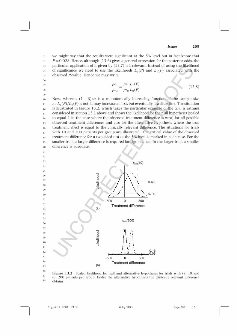
we might say that the results were significant at the 5% level but in fact know thatP = 0�028. Hence, although (13.6) gives a general expression for the posterior odds, theparticular application of it given by (13.7) is irrelevant. Instead of using the likelihoodof significance we need to use the likelihoods L1�P and L0�P associated with theobserved P-value. Hence we may write
po1
poo
= pr1
pr0
L1�P
L0�P(13.8)
Now, whereas �1 − �/ is a monotonically increasing function of the sample sizen� L1�P/L0�P is not. It may increase at first, but eventually it will decline. The situationis illustrated in Figure 13.2, which takes the particular example of the trial is asthmaconsidered in section 13.1 above and shows the likelihood for the null hypothesis (scaledto equal 1 in the case where the observed treatment difference is zero) for all possibleobserved treatment differences and also for the alternative hypothesis where the truetreatment effect is equal to the clinically relevant difference. The situations for trialswith 10 and 200 patients per group are illustrated. The critical value of the observedtreatment difference for a two-sided test at the 5% level is marked in each case. For thesmaller trial, a larger difference is required for significance. In the larger trial, a smallerdifference is adequate.
1
Treatment difference
Like
lihoo
d
0.15
0.63
xcrit(10)
xcrit(200)
1
0.050.15
–500 0
(a)
(b)
500
Treatment difference
Like
lihoo
d
–500 0 500
Figure 13.2 Scaled likelihood for null and alternative hypotheses for trials with (a) 10 and(b) 200 patients per group. Under the alternative hypothesis the clinically relevant differenceobtains.

01
02
03
04
05
06
07
08
09
10
11
12
13
14
15
16
17
18
19
20
21
22
23
24
25
26
27
28
29
30
31
32
33
34
35
36
37
38
39
40
41
42
43
44
45
46
47
48
August 14, 2007 21:30 Wiley/SIDD Page-206 c13
206 Determining the Sample Size
Note that the scaled likelihood for H0 is the same in both cases and approximatelyequal to 0.15. However, in the first case the likelihood is more than four times as highunder H1, being equal to 0.63, and in the second case only a third as high under H1,being equal to 0.05. Hence a given P-value of exactly 0.05 would provide evidencein favour of the alternative hypothesis in the first case and against it in the second.Thus, on this interpretation, moderate significance from a large trial would actuallybe evidence for the null hypothesis. (Note that if one is told only that the result issignificant, it is the area under the curve to the right of the critical value which isrelevant, and this is much higher in the larger trial. This was the situation consideredin section 13.2.8 but is not the situation here.)
The fact that a conventionally significant result can give evidence in favour of thenull hypothesis is known as the Jeffreys–Lindley paradox (Bartlett, 1957; Lindley, 1957;Senn, 2001b). In practice, such a situation would hardly ever arise. This is becausea significant P-value is not very likely given the null hypothesis (this is the basicidea behind the significance test) and it is even less likely given the sort of alternativehypothesis illustrated. The point is rather that, given that this unusual situation hasoccurred, it actually gives more evidence in favour of the null hypothesis. It is oneargument, once a trial has reached a certain power, to reduce the level of significancerequired.
Again, however, one has to be very careful in interpreting this result. The diagramonly illustrates the alternative hypothesis corresponding to the clinically relevantdifference. But if this is the difference we should not like to miss, it does notfollow that it is the only difference we should like to find. There may be lowervalues of the treatment effect which are of interest and these will produce higherlikelihoods.
13.2.10 For a given P-value, the evidence against the null hypothesis isthe same whatever the size of the trial
This has been referred to as the alpha postulate. There is a sense in which this istrue also! Look at Figure 13.3. Here, instead of displaying the scaled likelihood forthat alternative hypothesis which corresponds to the clinically relevant difference, thealternative hypothesis for which the true treatment effect corresponds to the criticalvalue is illustrated. For P = 0�05, the ratio of this likelihood is the same for the trialwith 10 patients per group as for the trial with 200 as, indeed, it is for any trialwhatsoever. But we do not know which value of the alternative hypothesis is true ifthe null hypothesis is false. It thus follows that for a P-value of exactly 0.05, there isalways one value of the alternative hypothesis for which the likelihood is 1/0.15 ormore than six times as high as for the null hypothesis. The evidence in favour of thisalternative hypothesis (which hypothesis changes according to the size of the trial) isalways the same.
This is one interpretation of the significance test. It is the sceptic’s concession tothe gullible. The sceptic asserts the null hypothesis, because he doesn’t believe in theefficacy of treatment. The gullible believes exactly whatever the data tell him. He thusadopts as his presumed treatment effect whatever the observed mean difference is. Sincethe ratio of likelihoods in favour of this hypothesis will always be greater than 1, hewill always obtain evidence in favour of his hypothesis. All that the sceptic can do is

01
02
03
04
05
06
07
08
09
10
11
12
13
14
15
16
17
18
19
20
21
22
23
24
25
26
27
28
29
30
31
32
33
34
35
36
37
38
39
40
41
42
43
44
45
46
47
48
August 14, 2007 21:30 Wiley/SIDD Page-207 c13
Issues 207
–500
(a)
(b)
0.5
1
Treatment difference
Like
lihoo
dLi
kelih
ood
0.15
1
xcrit(10)
xcrit(200)
0.5
1
0.15
1
0 500
–500
Treatment difference0 500
Figure 13.3 Scaled likelihood for null and alternative hypotheses for (a) 10 and (b) 200 patientsper group. Under the alternative hypothesis the difference corresponding to the critical value ofthe test obtains.
counter this by explaining what the consequences of this sort of behaviour are. ‘If youregard odds of 6 to 1 for the best supported difference compared to the null hypothesisas being evidence in favour of a treatment effect, then in at least 1 in 20 trials wherethe treatment is useless you will conclude it is effective.’ On this interpretation, aconventionally significant result then becomes a minimal requirement for concludingefficacy of a treatment.
In my opinion, this is, the way that drug development usually works. Treatmentsare not registered unless a significant result is obtained. This is, however, generally aminimal requirement. Other information (treatment estimates, confidence intervals, theanalyses of other outcomes, the results of further trials) is presented and unless this isfavourable, the drug will not be registered.
The above discussions should serve as a warning, however: the evidential interpre-tations of P-values is a delicate matter (Senn, 2001b).

01
02
03
04
05
06
07
08
09
10
11
12
13
14
15
16
17
18
19
20
21
22
23
24
25
26
27
28
29
30
31
32
33
34
35
36
37
38
39
40
41
42
43
44
45
46
47
48
August 14, 2007 21:30 Wiley/SIDD Page-208 c13
208 Determining the Sample Size
13.2.11 The effect of the two-trials rule on sample size
If we are required to prove significance in two trials, as is usually believed to benecessary in phase III for a successful NDA application, then from the practical pointof view it may be the power of the combined requirement which is important, ratherthan that for individual trials. On the assumption that the trials are competent andthat the background planning has been carried out appropriately and that trial bytreatment interactions may be dismissed, then the power to detect the clinically relevantdifference in both of two trials, each with power 80%, is 64% since 0�8 × 0�8 = 0�64.This means that 1 − 0�64 = 0�36, or more than one-third, of such drug developmentprogrammes would fail in phase III for failure of one or both clinical trials on this basis.(This does not mean that one-third of drug developments will fail in phase III, sincemany drugs which survive that far may, indeed, have an effect which is superior tothe clinically relevant difference. On the other hand, there may be other reasons forfailure.) If it is desired to have 80% power overall, then it is necessary to run each trialwith 90% power since 0�9 × 0�9 � 0�80.
As explained in Chapter 12, however, the two-trials rule is not particularly logical.The alternative pooled-trials rule would actually require only 4/5 of the number ofpatients of the two-trials rule for an overall power of 80% and an overall size of 1/1600,which is what, effectively, the two-trials rule implies.
Clinically relevant difference: That which is used to justify the sample size butwill be claimed to have been used to find it.
13.2.12 The effect of multiple requirements
Cairns and Ruberg point out that the FDA requires that for registration of treatmentsfor senile dementia, both global cognitive function and overall assessment by physicianmust be significantly superior to placebo (Cairns and Ruberg, 1996). In Europe, athird additional requirement for ‘activities of daily living’ is made. This means thatto plan a trial of adequate sample size to meet these requirements one would needto use two (three in Europe) clinically relevant differences. One would also have toknow the correlation between the repeat measures. A conservative approach wouldbe to assume independence. In that case a sample size determination could be madefor each measure for 90% power (USA) or 93% power (Europe) and the largest ofall of these determinations taken. (The European requirement would arise because0�93 × 0�93 × 0�93 � 0�80). Comparing the resulting sample size to the largest thatwould be required for any one of the outcomes taken singly with 80% power, thisleads to a 31% increase for the USA and a 46% increase for Europe. Of course, thisis extreme. In practice these outcomes will be correlated and better approaches canbe used. Nevertheless there will be an increase in sample size required. This issue isdiscussed in some detail by Kieser et al. (2004).
Most statisticians are, of course, aware of the point and will be concerned aboutrequirements for multiple outcomes. What is sometimes overlooked, however, isthat a similar point arises if conclusions are required to be robust to a number of

01
02
03
04
05
06
07
08
09
10
11
12
13
14
15
16
17
18
19
20
21
22
23
24
25
26
27
28
29
30
31
32
33
34
35
36
37
38
39
40
41
42
43
44
45
46
47
48
August 14, 2007 21:30 Wiley/SIDD Page-209 c13
Issues 209
analyses: the Mann–Whitney–Wilcoxon test as well as the t-test, for example, orincluding or omitting various covariates. Such multiple requirements also lead to anincrease in the sample size needed. (Although, at a guess, the problem will not be assevere as for multiple outcomes.)
Such multiple requirements seem from one point of view to be a good thing. A strongerstandards of evidence overall is implicit and in the end we shall have greater confidencein the value of a registered drug. By the same token, however, the ethical problemswhich arise through sample size requirements can be aggravated by such requirements.In any case, the practical consideration is that the pharmaceutical statistician has tobecome aware of the requirements of conjunctive power, that is to say the need fortest 1 and test 2 and test 3, etc. (hence conjunctive) to be significant.
There is also one technical matter which is worth comment. Suppose we requirethat a t-test and a Mann–Whitney–Wilcoxon test both be significant at the 5% level.Let us call this the two-test procedure. These two tests are certainly highly correlatedso that the overall type I error rate will be somewhere between 0.05 (the value werethey perfectly correlated) and 0.0025 (the value were they independent). Suppose, forargument’s sake, that the value is 0.01. I suspect that for moderately sized trials theloss in power as a result of the double requirement, where Normality applies and eithertest could be used, will be small. Nevertheless, there will be some loss. Of course, thereis the gain that a higher standard of evidence of efficacy is required. However, a higherstandard of efficacy could be obtained simply by requiring that a t-test on its own besignificant at the 1% level. It would be interesting to see this requirement comparedformally with that of the two-test procedure.
For further discussion of the effect of multiple outcomes on power see Chuang-Steinet al. (2007), Offen et al. (2007) and Senn and Bretz (2007).
13.2.13 In order to interpret a trial it is necessary to know its power
This is a rather silly point of view that nevertheless continues to attract adherents. Apower calculation is used for planning trials and is effectively superseded once the dataare in. For an impression of the precision of the result, one is best looking at confidenceintervals or standard errors. If the result is significant, then to the extent that oneaccepts the logic of significance tests, there is no point arguing about the result. Ananalogy may be made. In determining to cross the Atlantic it is important to considerwhat size of boat it is prudent to employ. If one sets sail from Plymouth and severaldays later sees the Statue of Liberty and the Empire State Building, the fact that theboat employed was rather small is scarcely relevant to deciding whether the Atlanticwas crossed.
Retrospective power calculations are sometimes encountered for so-called failed trials,but this seems particularly pointless. The clinically relevant difference does not changeas a result of having run the trial, in which case the power is just a function of theobserved variance. It says nothing about the effect of treatment.
Some check-lists for clinical trials seem to require evidence that a power calculationwas performed, but this surely can have very little relevance to the interpretation of thefinal result. At best it can be a very weak indicator of the quality of the study.
For a trenchant criticism of the use of retrospective power calculations see Hoenigand Heisey (2001).

01
02
03
04
05
06
07
08
09
10
11
12
13
14
15
16
17
18
19
20
21
22
23
24
25
26
27
28
29
30
31
32
33
34
35
36
37
38
39
40
41
42
43
44
45
46
47
48
August 14, 2007 21:30 Wiley/SIDD Page-210 c13
210 Determining the Sample Size
13.2.14 The dimension of cost
A very unsatisfactory feature of conventional approaches to sample size calculation isthat there is no mention of cost. This means that for any two quite different indicationswith the same effect size, that is to say the same ratio of clinically relevant difference tostandard deviation, the sample size would be the same whatever the cost or difficulty ofrecruiting and treating patients. This is clearly illogical and trialists probably managethis issue informally by manipulating the clinically relevant difference in way discussedin Section 13.2.3. Clearly, it would be better to include the cost explicitly, and thissuggests decision-analytic approaches to sample size determination. There are variousBayesian suggestions and these will be discussed in the next section.
13.2.15 Bayesian approaches to sample size determination
A Bayesian approach to sample size determination may be discussed in terms of a ratherartificial and not very realistic case, namely that where a single phase III study must berun in a nonsequential manner and on the basis of this the treatment will be registeredor not. Now consider a trial of a given sample size and suppose that a decision will bemade on the basis of a statistic from such a trial. Suppose that it is known for everyvalue of the statistic whether the regulator will register the drug or not and that a lossmay be associated with failing to register. Of course, the regulator’s decision might itselfbe based on a suitable loss function and prior distribution, but from the sponsor’s pointof view this does not matter provided only that the decision that will be taken is known.
Now, given a suitable prior distribution (which does not have to be the same as theregulator’s), the sponsor can calculate the predictive distribution for the test statistic andhence the expected loss for any given sample size, including the cost of experimentation.The optimal sample size is then the one with the smallest expected loss. This is a doubleoptimization procedure: the optimal decision (minimum loss) for a given value of thetest statistic and sample size must be determined and then the sample size which yieldsthe smallest minimum loss is chosen (Lindley, 1997).
Various Bayesian approaches that have been suggested are variants of this. Forexample, Lindley’s approach (Lindley, 1997) involves a sophisticated use of loss func-tions and is fully Bayesian but applies when regulator and sponsor have the same beliefsand values. That of Gittins and Pezeshk is a hybrid Bayes-frequentist system in whichit is supposed that eventual sales of a pharmaceutical are a function of how impres-sive the trial results are (measured by conventional significance) but that in planning,prior distributions and a Bayesian approach are used (Gittins and Pezeshk, 2000a,b;Pezeshk and Gittins, 2002). For an implementation in SAS of a simpler approach withcosts per patient but a single reward for a significant trial, see Burman et al. (2007).This uses a prior distribution on the treatment effect. Application of this in a hybridBayesian/frequentist approach is discussed in Section 13.2.16.
13.2.16 An appropriate approach to sample size determination is tocalculate assurance
Even closer to a frequentist approach than the methods of Section 13.2.15 is that ofcalculating what O’Hagan et al. call assurance (O’Hagan et al., 2005). This is the

01
02
03
04
05
06
07
08
09
10
11
12
13
14
15
16
17
18
19
20
21
22
23
24
25
26
27
28
29
30
31
32
33
34
35
36
37
38
39
40
41
42
43
44
45
46
47
48
August 14, 2007 21:30 Wiley/SIDD Page-211 c13
Issues 211
Bayesian probability of a clinical trial yielding a significant result. Rather than beingconditional on a particular posited clinically relevant difference, it uses a prior distri-bution for the treatment effect and integrates the conventional frequentist power overthis distribution to obtain an unconditional expected power, assurance. If this approachalone is used for sample size determination it means that the clinically relevant differ-ence has no role whatsoever in determining how large the trial should be. As suggestedin Section 13.2.14, conventional power calculations are already unsatisfactory in thatthey treat identically two indications with differing costs but identical effect sizes. Assur-ance, however, seems to take this one stage further. Provided that the prior distributionsfor treatment effects for two indications are the same and the precision is the same,then if assurance is to be the guide, the sample sizes will be the same, even if in termsof practical interest the prior distributions are quite different.
For this and other reasons, I am not particularly keen on the use of assurance asthe primary criterion for designing a clinical trial, although it may well be useful tocalculate it in addition. My own view is that if I am going to be Bayesian about samplesize calculation I would rather be hanged for a sheep than a lamb and use the methodsof section 13.2.15.
References
Altman DG, Bland JM (1995) Absence of evidence is not evidence of absence. British MedicalJournal 311: 485.
Bartlett MS (1957) A comment on D.V. Lindley’s statistical paradox. Biometrika 44: 533–534.Burman C-F, Grieve AP, Senn S (2007) Decision analysis in drug development. In: Dmitrienko
A, Chuang-Stein C, Agostino R (eds), Pharmaceutical Statistics Using SAS: A Practical Guide. SASInstitute, Cary, pp. 385–428.
Cairns V, Ruberg S (1996) The confirmatory package of trials–design. In: Jones B, Teather B,Teather D (eds), Proceedings of Statistical Issues in Biopharmaceutical Environments: USA andEuropean Perspectives, De Monfort University, Leicester.
Chuang-Stein C, Stryszak P, Dmitrienko A, Offen W (2007) Challenge of multiple co-primaryendpoints: a new approach. Statistics in Medicine 26: 1181–1192.
Committee for Proprietary Medicinal Products (1995) Note for guidance on the clinical investigationof medicinal products in the treatment of chronic peripheral arterial occlusive disease. EMEA, London.http://www.emea.europa.eu/pdfs/human/ewp/071498eu.pdf.
Desu MM, Raghavarao D (1990) Sample Size Methodology. Academic Press, Boston.Edwards SJ, Lilford RJ, Braunholtz D, Jackson J (1997) Why ‘underpowered’ trials are not neces-
sarily unethical [see comments]. Lancet 350: 804–807.Gittins J, Pezeshk H (2000a) A behavioral Bayes method for determining the size of a clinical
trial. Drug Information Journal 34: 355–363.Gittins J, Pezeshk H (2000b) How large should a clinical trial be? Journal of the Royal Statistical
Society Series D–The Statistician 49: 177–187.Hoenig JM, Heisey DM (2001) The abuse of power: the pervasive fallacy of power calculations
for data analysis. American Statistician 55: 19–24.Julious SA (2004) Tutorial in biostatistics–Sample sizes for clinical trials with normal data.
Statistics in Medicine 23: 1921–1986.Julious SA (2006) Designing clinical trials with uncertain estimates of variability. PhD, University
College London, London.Kieser M, Röhmel J, Friede T (2004) Power and sample size determination when assessing the
clinical relevance of trial results by ‘responder analyses’. Statistics in Medicine 23: 3287–3305.Lindley DV (1957) A statistical paradox. Biometrika 44: 187–192.

01
02
03
04
05
06
07
08
09
10
11
12
13
14
15
16
17
18
19
20
21
22
23
24
25
26
27
28
29
30
31
32
33
34
35
36
37
38
39
40
41
42
43
44
45
46
47
48
August 14, 2007 21:30 Wiley/SIDD Page-212 c13
212 Determining the Sample Size
Lindley DV (1997) The choice of sample size. Statistician 46: 129–138.O’Hagan A, Stevens JW, Campbell MJ (2005) Assurance in clinical trial design. Pharmaceutical
Statistics 4: 186–201.Offen W, Chuang-Stein C, Dmitrienko A, et al. (2007) Multiple co-primary endpoints: medical and
statistical solutions–A report from the Multiple Endpoints Expert Team of the PharmaceuticalResearch and Manufacturers of America. Drug Information Journal 41: 31–46.
Pezeshk H, Gittins J (2002) A fully Bayesian approach to calculating sample sizes for clinicaltrials with binary responses. Drug Information Journal 36: 143–150.
Royall RM (1986) The effect of sample size on the meaning of significance tests. The AmericanStatistician 40: 313–315.
Ruberg S, Cairns V (1998) Providing evidence of efficacy for a new drug. Statistics in Medicine17: 1813–1823.
Senn SJ (2001a) The misunderstood placebo. Applied Clinical Trials 10: 40–46.Senn SJ (2001b) Two cheers for P-values. Journal of Epidemiology and Biostatistics 6: 193–204.Senn SJ (2002) Ethical considerations concerning treatment allocation in drug development trials.
Statistical Methods in Medical Research 11: 403–411.Senn SJ, Bretz F (2007) Power and sample size when multiple endpoints are considered. Pharma-
ceutical Statistics. [In press].