Embed Size (px)
Citation preview

13: Linear Equalization
LINEAR EQUALIZATION
⋆ Multipath and Other Interference
⋆ Trained Least-Squares Linear Equalization
⋆ Trained Adaptive Least-Mean-Square Equalization
⋆ Blind Adaptive Decision-Directed Equalization
⋆ Blind Adaptive Dispersion Minimizing Equalization
adaptive components
Software Receiver Design Johnson/Sethares/Klein 1 / 36

13: Linear Equalization
Multipath and Other Interference
◮ Assume up and down conversion and carrier and clock recovery(including matched filtering and downsampling) all executedtransparently.
◮ Impairment of interest is multipath interference (linear filtering byanalog channel and receiver front-end preceding equalizer) and otheradditive interference (broadband noise and narrowband interferers).
Pulse shaping
Analog channel
Decision device
Linear digital
equalizer
Digital source
Received analog signal
Received analog signal
Sampled received
signal
Noise and interferers
T
1
Software Receiver Design Johnson/Sethares/Klein 2 / 36

13: Linear Equalization
Multipath ... Interference (cont’d)
◮ FIR channel model:
y(kT ) = a1u(kT ) + a2u((k − 1)T )
+ . . .+ anu((k − n)T ) + η(kT )
where η(kT ) is sample of other interference.
◮ Order n of discrete-time FIR channel model dependent on physicaldelay spread of channel.
◮ For 4 µsec delay spread by “physical” channel:
⊙ T = 0.04 µsec → 25 Msymbols/sec → n = 100⊙ T = 0.4 µsec → 2.5 Msymbols/sec → n = 10⊙ T = 4 µsec → 0.25 Msymbols/sec → n = 1
Software Receiver Design Johnson/Sethares/Klein 3 / 36

13: Linear Equalization
Multipath ... Interference (cont’d)
◮ Multipath FIR model coefficients depend on actual baud-timingchoice of clock recovery algorithm, which need not match timing innon-ISI situation.
◮ Example: Two-ray analog channel c(t) = p(t) + 0.6p(t−∆) with∆ = 0.7T
0
Lattice of Ts-spaced optimal sampling times with ISI
p(t)
0.6 p(t 2 D)
c(t) 5 p(t) 1 0.6 p(t 2 D)
Lattice of Ts-spaced optimal sampling times with no ISI
Sum of received pulses
The digital channel model is given by Ts-spaced
samples of c(t) Software Receiver Design Johnson/Sethares/Klein 4 / 36

13: Linear Equalization
Trained Least-Squares Linear Equalization
◮ Objective: Choose impulse response f of equalizer so y[k] ≈ s[k − δ](so e ≈ 0) for some δ.
Source s[k]
Channel Equalizer
Additive interferers
Delay
Impulse response f
Received signal r[k]
Training signalError e[k]2
Equalizer output y[k]
1
1
◮ Equalizer Output: y[k] =∑n
j=0 fjr[k − j]
y[k]
r[k]z21 z21 z21
f0 f1 fn
. . .
. . .
1 1
Software Receiver Design Johnson/Sethares/Klein 5 / 36

13: Linear Equalization
Trained ... Equalization (cont’d)
◮ Write equalizer output for k = n+ 1 as inner product
y[n+ 1] = [r[n+ 1], r[n], ..., r[1]]
f0f1...fn
◮ Similarly, for k = n+ 2
y[n+ 2] = [r[n+ 2], r[n+ 1], ..., r[2]]
f0f1...fn
Software Receiver Design Johnson/Sethares/Klein 6 / 36

13: Linear Equalization
Trained ... Equalization (cont’d)
Concatenating these equations for k = n+ 1 to p
y[n+ 1]y[n+ 2]y[n+ 3]
...y[p]
=
r[n+ 1] r[n] ... r[1]r[n+ 2] r[n+ 1] ... r[2]r[n+ 3] r[n+ 2] ... r[3]
......
...r[p] r[p− 1] ... r[p− n]
f0f1...fn
or with appropriate definitions
Y = RF
where R with its diagonal stripes of repeated values is a Toeplitz matrix.
Software Receiver Design Johnson/Sethares/Klein 7 / 36

13: Linear Equalization
Trained ... Equalization (cont’d)
Delayed source recovery error:
e[k] = s[k − δ]− y[k]
Delayed source vector:
S =
s[n+ 1− δ]s[n+ 2− δ]s[n+ 3− δ]
...s[p− δ]
Error vector:
E =
e[n+ 1]e[n+ 2]e[n+ 3]
...e[p]
= S − Y = S −RFSoftware Receiver Design Johnson/Sethares/Klein 8 / 36

13: Linear Equalization
Trained ... Equalization (cont’d)
Average squared delayed source recovery error:
J̄ =
(
1
p− n
) p∑
i=n+1
e2[i]
Summed squared error:
J =∑p
i=n+1 e2[i]
= ETE
= (S −RF )T (S −RF )
= STS − (RF )TS − STRF + (RF )TRF
Because J is a scalar, (RF )TS and STRF are scalars and
(RF )TS = ((RF )TS)T = ST ((RF )T )T = STRF
soJ = STS − 2STRF + (RF )TRF
Software Receiver Design Johnson/Sethares/Klein 9 / 36

13: Linear Equalization
Trained ... Equalization (cont’d)
◮ Define
Ψ , [F − (RTR)−1RTS]T (RTR) · [F − (RTR)−1RTS]
= F T (RTR)F − STRF − F TRTS + STR(RTR)−1RTS
◮ Rewrite J as
J = Ψ+ STS − STR(RTR)−1RTS
= Ψ+ ST [I −R(RTR)−1RT ]S
◮ Because the term ST [I −R(RTR)−1RT ]S is not a function of F , theminimum of J by choice of F occurs at the F that minimizes Ψ, i.e.
F ∗ = (RTR)−1RTS
assuming (RTR)−1 exists.
Software Receiver Design Johnson/Sethares/Klein 10 / 36
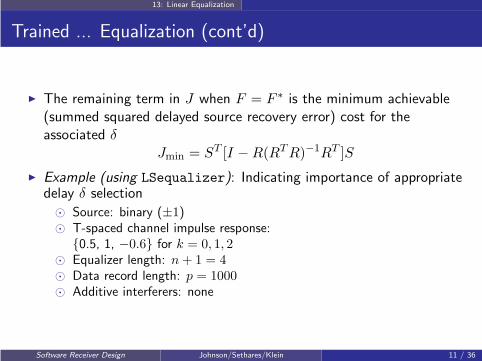
13: Linear Equalization
Trained ... Equalization (cont’d)
◮ The remaining term in J when F = F ∗ is the minimum achievable(summed squared delayed source recovery error) cost for theassociated δ
Jmin = ST [I −R(RTR)−1RT ]S
◮ Example (using LSequalizer): Indicating importance of appropriatedelay δ selection
⊙ Source: binary (±1)⊙ T-spaced channel impulse response:
{0.5, 1, −0.6} for k = 0, 1, 2⊙ Equalizer length: n+ 1 = 4⊙ Data record length: p = 1000⊙ Additive interferers: none
Software Receiver Design Johnson/Sethares/Klein 11 / 36

13: Linear Equalization
Trained ... Equalization (cont’d)
◮ Example (cont’d)
⊙ Results:δ Jmin F ∗
0 832 {0.33, 0.027, 0.070, 0.01}1 134 {0.66, 0.36, 0.16, 0.08}2 30 {−0.28, 0.65, 0.30, 0.14}3 45 {0.1, −0.27, 0.64, 0.3}
⊙ Smallest Jmin for δ = 2⊙ All δ except δ = 0 result in open eye and no decision errors.
Software Receiver Design Johnson/Sethares/Klein 12 / 36

13: Linear Equalization
Trained ... Equalization (cont’d)
Another Example:
◮ Equalizer: y[k] = f0r[k] + f1r[k − 1]
◮ Received signal data set:
{r[k]} = {r[1], r[2], r[3], r[4], r[5]}
◮ Source signal data set:
{s[k]} = {s[1], s[2], s[3], s[4], s[5]}
◮ Zero-delay objective: y[k] ∼ s[k]. The largest collection of equationsavailable from dataset is
s[2]s[3]s[4]s[5]
∼
r[2] r[1]r[3] r[2]r[4] r[3]r[5] r[4]
[
f0f1
]
Software Receiver Design Johnson/Sethares/Klein 13 / 36

13: Linear Equalization
Trained ... Equalization (cont’d)
Another Example (cont’d):
◮ δ = 1 objective: y[k] ∼ s[k − 1]. The largest collection of equationsavailable from dataset is
s[1]s[2]s[3]s[4]
∼
r[2] r[1]r[3] r[2]r[4] r[3]r[5] r[4]
[
f0f1
]
◮ δ = 2 objective: y[k] ∼ s[k − 2]. The largest collection of equationsavailable from dataset is
s[1]s[2]s[3]
∼
r[3] r[2]r[4] r[3]r[5] r[4]
[
f0f1
]
Software Receiver Design Johnson/Sethares/Klein 14 / 36
13: Linear Equalization
Trained ... Equalization (cont’d)
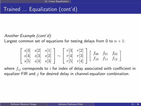
Another Example (cont’d):Largest common set of equations for testing delays from 0 to n+ 1:
s[3] s[2] s[1]s[4] s[3] s[2]s[5] s[4] s[3]
∼
r[3] r[2]r[4] r[3]r[5] r[4]
[
f00 f01 f02f10 f11 f12
]
where fij corresponds to i for index of delay associated with coefficient inequalizer FIR and j for desired delay in channel-equalizer combination.
Software Receiver Design Johnson/Sethares/Klein 15 / 36

13: Linear Equalization
Trained ... Equalization (cont’d)
Another Example (cont’d):All together now... S̄ ∼ R̄F̄ with
S̄ =
s[α+ 1] s[α] ... s[1]s[α+ 2] s[α+ 1] ... s[2]
......
...s[p] s[p− 1] ... s[p− α]
R̄ =
r[α+ 1] r[α] ... r[α− n+ 1]r[α+ 2] r[α+ 1] ... r[α− n+ 2]
......
...r[p] r[p− 1] ... r[p− n]
F̄ =
f00 f01 ... f0αf10 f11 ... f1α...
......
fn0 fn1 ... fnα
Software Receiver Design Johnson/Sethares/Klein 16 / 36
13: Linear Equalization
Trained ... Equalization (cont’d)
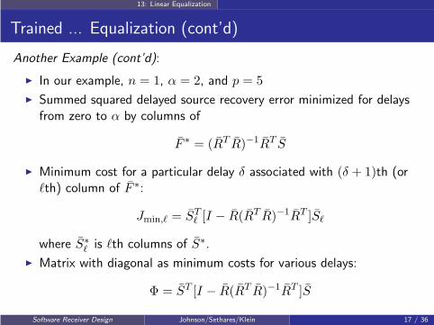
Another Example (cont’d):
◮ In our example, n = 1, α = 2, and p = 5
◮ Summed squared delayed source recovery error minimized for delaysfrom zero to α by columns of
F̄ ∗ = (R̄T R̄)−1R̄T S̄
◮ Minimum cost for a particular delay δ associated with (δ + 1)th (orℓth) column of F̄ ∗:
Jmin,ℓ = S̄Tℓ [I − R̄(R̄T R̄)−1R̄T ]S̄ℓ
where S̄∗
ℓ is ℓth columns of S̄∗.
◮ Matrix with diagonal as minimum costs for various delays:
Φ = S̄T [I − R̄(R̄T R̄)−1R̄T ]S̄
Software Receiver Design Johnson/Sethares/Klein 17 / 36

13: Linear Equalization
Trained ... Equalization (cont’d)
The steps of the linear FIR equalizer design strategy are:
1. Select the order n for the FIR equalizer.
2. Select maximum of candidate delays α (> n).
3. Utilize set of p training signal samples {s[1], s[2], ..., s[p]} withp > n+ α.
4. Obtain corresponding set of p received signal samples{r[1], r[2], ..., r[p]}.
5. Compose S̄.
6. Compose R̄.
7. Check if R̄T R̄ has poor conditioning induced by any (near) zeroeigenvalues.
8. Compute F̄ ∗.
9. Compute Φ = S̄T [S̄ − R̄F̄ ∗].
Software Receiver Design Johnson/Sethares/Klein 18 / 36

13: Linear Equalization
Trained ... Equalization (cont’d)
Equalizer design strategy (cont’d):
10. Find the minimum value on the diagonal of Φ. This index is δ + 1.The associated diagonal element of Φ is the minimum achievablesummed squared delayed source recovery error
∑
i e2[i] over the
available data record.
11. Extract the (δ + 1)th column of the previously computed F̄ ∗. This isthe impulse response of the optimum equalizer.
12. Test the design. Test it on synthetic data, and then on measureddata (if available). If inadequate, repeat design, perhaps increasing nor twiddling some other designer-selected quantity.
Software Receiver Design Johnson/Sethares/Klein 19 / 36

13: Linear Equalization
Trained ... Equalization (cont’d)
Complex Signals:
◮ For modulations such as QAM, the signals (and parameters) areeffectively complex valued.
◮ For a complex error e[k] = eR[k] + jeI [k] where j =√−1, consider
e[k]e∗[k] where ∗ superscript indicates complex conjugation.
◮ The coste[k]e∗[k] = e2R[k]− jeR[k]eI [k]
+jeR[k]eI [k]− j2e2I [k]
= e2R[k] + e2I [k]
is desirably nonnegative.
◮ Optimal equalizer to minimize∑
k e[k]e∗[k] is
F ∗ = (RHR)−1RHS
where superscript H denotes transposition and complex conjugation.
Software Receiver Design Johnson/Sethares/Klein 20 / 36

13: Linear Equalization
Trained ... Equalization (cont’d)
Fractionally-Spaced Equalizer:
◮ For an equalizer with an input sampled M times per symbol period,we wish to minimize the square of e only at the the baud times,i.e. every M th sample (with synchronized sampler).
◮ Thus, only every M th e in E matters, and the underlying equationsof interest are the rows of E = S −RF left after removing all butevery M th one.
◮ The remaining matrix equation is solved, which can admit a perfectsolution if the row-decimated R has been reduced to a square matrix.
Software Receiver Design Johnson/Sethares/Klein 21 / 36

13: Linear Equalization
Trained Adaptive Least-Mean-Square (LMS) Equalization
We choose to minimize
avg{e2[k]} = 1N
∑k0+N−1k=k0
e2[k]
with e[k] = s[k − δ]−∑ni=0 fir[k − i] using a gradient descent scheme
fi[k + 1] = fi[k]− µ̄∂(avg{e2[k]})
∂fi|f=f [k]
With differentiation and average approximately commutable (see App. G)
fi[k + 1] ≈ fi[k]− µ̄ · avg{
∂e2[k]
∂fi|f=f [k]
}
Dropping the “outer” average produces LMS
fi[k + 1] = fi[k]− 2µ̄
(
e[k]∂e[k]
∂fi
)
|f=f [k]
= fi[k] + µ(s[k − δ]− y[k])r[k − i]
with y[k] =∑n
j=0 fj [k]r[k − j].
Software Receiver Design Johnson/Sethares/Klein 22 / 36

13: Linear Equalization
Trained Adaptive Least-Mean-Square (LMS) Equalization(cont’d)
With the definition of the FIR equalizer output
y[k] =n∑
j=0
fj [k]r[k − j]
in
f [k] Sign[·]
r[k] y[k]
e[k] s[k] training signal
Equalizer
Adaptive algorithm
Performance evaluation
Decision device
Sampled received signal
the trained approximate gradient descent adaptation algorithm LMS forthe linear equalizer is
fi[k + 1] = fi[k] + µ(s[k − δ]− y[k])r[k − i]
Software Receiver Design Johnson/Sethares/Klein 23 / 36

13: Linear Equalization
Blind Adaptive Decision-Directed Equalization
We choose to minimize
avg{(Q(n∑
j=0
fjr[k − j])−n∑
j=0
fjr[k − j])2}
=1
N
k0+N−1∑
k=k0
(Q(
n∑
j=0
fjr[k − j])−n∑
j=0
fjr[k − j])2
using a gradient descent scheme
fi[k + 1] = fi[k]− µ̄∂
∂fi
avg{(Q(
n∑
j=0
fjr[k − j])
−n∑
j=0
fjr[k − j])2}
|f=f [k]
Software Receiver Design Johnson/Sethares/Klein 24 / 36

13: Linear Equalization
Blind Adaptive Decision-Directed Equalization (cont’d)
Commute average and partial derivative, drop “outer” average, andpresume ∂(Q(
∑nj=0 fjr[k − j]))/∂fi = 0 to produce
fi[k + 1] = fi[k]− 2µ̄{(Q(n∑
j=0
fjr[k − j])
−n∑
j=0
fjr[k − j])∂(−∑n
j=0 fjr[k − j])
∂fi}|f=f [k]
= fi[k]− 2µ̄
Q(n∑
j=0
fj [k]r[k − j])
−n∑
j=0
fj [k]r[k − j]
(−r[k − i])
Software Receiver Design Johnson/Sethares/Klein 25 / 36

13: Linear Equalization
Blind ... Equalization (cont’d)
With the definition of
y[k] =∑n
j=0 fj [k]r[k − j]
in
f [k] Sign[·]
r[k] y[k]
e[k]
Equalizer
Adaptive algorithm
Performance evaluation
Decision device
Sampled received signal
the decision-directed approximate gradient descent adaptation algorithmfor the linear FIR equalizer is
fi[k] = fi[k] + µ(Q(y[k])− y[k])r[k − i]
◮ Relative to trained adaptation via LMS, the decision device outputjust replaces the training signal.
Software Receiver Design Johnson/Sethares/Klein 26 / 36

13: Linear Equalization
Blind Adaptive Dispersion-Minimizing Equalization
We choose to minimize
avg{(1− (n∑
j=0
fjr[k − j])2)2} =1
N
k0+N−1∑
k=k0
(1− (n∑
j=0
fjr[k − j])2)2
using a gradient descent scheme
fi[k + 1] = fi[k]− µ̄∂(
avg{(1− (∑n
j=0 fjr[k − j])2)2})
∂fi|f=f [k]
Commuting average and differentiation and dropping “outer” averageproduces
fi[k + 1] = fi[k] + 2µ̄{(1− (n∑
j=0
fjr[k − j])2)
·∂(∑n
j=0 fjr[k − j])2
∂fi}|f=f [k]
Software Receiver Design Johnson/Sethares/Klein 27 / 36

13: Linear Equalization
Blind ... Equalization (cont’d)
Evaluating derivative produces
fi[k + 1] = fi[k] + µ(1− (n∑
j=0
fj [k]r[k − j])2) · (n∑
j=0
fj [k]r[k − j])r[k − i]
wheren∑
j=0
fj [k]r[k − j] = y[k]
sofi[k + 1] = fi[k] + µ(1− y2[k])y[k]r[k − i]
In comparison to LMS the prediction error s[k − δ]− y[k] has beeneffectively replaced by (1− y2[k])y[k].
Software Receiver Design Johnson/Sethares/Klein 28 / 36

13: Linear Equalization
Blind ... Equalization (cont’d)
With the definition of
y[k] =∑n
j=0 fj [k]r[k − j]
in
r[k] y[k]
e[k]
Equalizer
Adaptive algorithm
Sampled received
signal
X2
g
y2[k]
Performance evaluation
12
the dispersion-minimizing approximate gradient descent adaptationalgorithm for the linear FIR equalizer is
fi[k + 1] = fi[k] + µ(1− y2[k])y[k]r[k − i]
◮ The adaptive scheme is labelled as blind (rather than trained) due tothe creation of the correction term without a training signal.
Software Receiver Design Johnson/Sethares/Klein 29 / 36

13: Linear Equalization
Example (using dae)
◮ Source: binary (±1)
◮ Channel:
⊙ Zero: {1 .9 .81 .73 .64 .55 .46 .37 .28}/4.138⊙ One: {1 1 1 0.2 -0.4 2 -1}/8.2⊙ Two: {-0.2 .1 .3 1 1.2 .4 -.3 -.2 .3 .1 -.1}/2.98
◮ Sinusoidal interferer frequency: 1.4 radians/sample
◮ Some broadband noise present
◮ Equalizer length: 33
Software Receiver Design Johnson/Sethares/Klein 30 / 36

13: Linear Equalization
Example (cont’d)
Trained LS for channel zero:
0
20.5
21
0.5
0 1000 2000 3000 4000
1
0.8
0.4
0.6
0.2
0
20.2
1
0 10 20 30 40
1.2
0
21
22
1
0 1000 2000 3000 4000
2
Decision device recovery error
0
0.5
20.5
21.5
21
1
220 1000 2000 3000 4000
1.5
Combined channel and optimal equalizer impulse response
Optimal equalizer outputReceived signal
230
250
260
210
220
240
0
0 1 2 3 4
10
0
0.5
20.5
21
1
21 0 1
0
210
220
10
0 1 2 3 4
20
Freq Resp Phase
20.5
0
0.5
2121 020.5 0.5 1
1
Zeros of channel/equalizer combination
Freq Resp Magnitude
Normalized frequency
FIR channel zeros
Imagin
ary
part
Imagin
ary
part
db
rad
ian
s
Real part
Normalized frequencyReal part
Software Receiver Design Johnson/Sethares/Klein 31 / 36

13: Linear Equalization
Example (cont’d)
Trained LS for channel one:
0 1000 2000 3000 400021
20.5
0
0.5
1
Received signal
0 1000 2000 3000 4000
Optimal equalizer output
21.5
21
20.5
0
0.5
1.5
1
0 10 20 30 40
Combined channel and optimal equalizer impulse response
0 1000 2000 3000 4000
Decision device recovery error
21
20.5
0
0.5
1
20.2
0.2
0.6
0
0.4
0.8
1
1.2
21 0 1
FIR channel zeros
0 1 2 3 4
Freq Resp Magnitude
Zeros of channel/equalizer combination
0 1 2 3 4
Freq Resp Phase
Normalized frequency
rad
ian
sd
b
Normalized frequency
Real part
Real part
Imagin
ary
part
Imagin
ary
part
240
230
220
210
0
21
20.5
0.5
0
1
220
210
0
10
20
22
24
0
2
4
210 28 26 24 22 0
Software Receiver Design Johnson/Sethares/Klein 32 / 36

13: Linear Equalization
Example (cont’d)
Trained LS for channel two:
1.5
1
0.5
0
20.5
21
21.50 1000 2000 3000 4000
Received signal
1.2
1
0.8
0.6
0.2
0.4
0
1
0.5
0
20.5
2120.20 0 1000 2000 3000 400010 20 30 40 50
Combined channel and optimal equalizer impulse response
1.5
1
0.5
0
20.5
21.5
21
220 1000 2000 3000 4000
Optimal equalizer output
Decision device recovery error
1.5
1
0.5
0
20.5
21
21.521 0 1 2
FIR channel zeros
Real part
Imagin
ary
part
db
0
210
215
25
220
225
230
2350 1 2 3 4
Zeros of channel/equalizer combination
30
20
10
0
210
230
220
0 1 2 3 4
Freq Resp Magnitude
Normalized frequency
Normalized frequency
Freq Resp Phase
1.5
1
0.5
0
20.5
21
21.521 0 1 2
Real part
Imagin
ary
part
rad
ian
sSoftware Receiver Design Johnson/Sethares/Klein 33 / 36

13: Linear Equalization
Example (cont’d)
Trained LMS for channel zero:
25
210
215
0
0 1 2 3 4
5
Normalized frequency
0
21
22
23
1
0 1000 2000 3000 4000
2
Iterations
dB
Ad
ap
tive e
qu
ali
zer
ou
tpu
t
2
1.5
1
0.5
0
2.5
0 1000 2000 3000 4000
3
Iterations
Combined magnitude response
100
1021
0 1000 2000 3000 4000
101
Iterations
Sq
uare
d p
red
icti
on
err
or
Su
mm
ed
sq
uare
d p
ara
mete
r err
or
Software Receiver Design Johnson/Sethares/Klein 34 / 36

13: Linear Equalization
Example (cont’d)
Decision-directed for channel zero:
25
210
215
0
0 1 2 3 4
5
Normalized frequency
1
0
21
22
23
2
0 1000 2000 3000 4000
3
Iterations
dB
Ad
ap
tive e
qu
ali
zer
ou
tpu
t
1
0.5
0
1.5
0 1000 2000 3000 4000
2
Iterations
Combined magnitude response
100
1021
0 1000 2000 3000 4000
101
Iterations
Sq
uare
d p
red
icti
on
err
or
Su
mm
ed
sq
uare
d p
ara
mete
r err
or
Software Receiver Design Johnson/Sethares/Klein 35 / 36
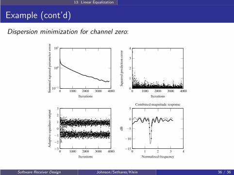
13: Linear Equalization
Example (cont’d)
Dispersion minimization for channel zero:
25
210
215
0
0 1 2 3 4
5
Normalized frequency
1
0
21
22
23
2
0 1000 2000 3000 4000
3
Iterations
dB
Ad
ap
tive e
qu
ali
zer
ou
tpu
t
2
1
0
3
0 1000 2000 3000 4000
4
Iterations
Combined magnitude response
100
1021
0 1000 2000 3000 4000
101
Iterations
Sq
uare
d p
red
icti
on
err
or
Su
mm
ed
sq
uare
d p
ara
mete
r err
or
Software Receiver Design Johnson/Sethares/Klein 36 / 36


![Chapter 13 Introduction to Statistical Quality Control ...noordin/s/ch13 rev.pdf · Title: Microsoft PowerPoint - ch13 rev [Compatibility Mode] Author: noordin Created Date: 10/15/2012](https://img.pdfslide.net/doc/110x75/60359a345d870e59ed2713cb/chapter-13-introduction-to-statistical-quality-control-noordinsch13-revpdf.jpg)