35 131 FINAL REPORT ON CONTRAICT F492-S5-C-W26 VOLUME 3(U) 1/1lPRINCETON UNly NJ DEPT OF MECNRNICAL AMO FA0OPACENGINEERING S R ORSZRG MAY 87 RFOSR-TR-67-1349-VOL-3

UNCL SIFIDF4 U235-C-26SMFA 20/4 I.

EEEmohEohEEshhEsmmhhEEEmhEmhhEhhmhEEEEEEEEIsmmhEEEEmhhhEEmEEEEI.EmmoEI

11111 1.05

11LO1 11122ONT[ICHRDLAsUN, q j -i I N PLl

'Iii:;%

%4 %IIL11111~J -A III

AFOSR-Tit. 8 7 - I S,

UIJIE COPY

* CV)

LOl00 FINAL REPORT ON

* AFOSR CONTRACT F49620-85-C-0026

I Steven A. Orszag, Principal InvestigatorDepartment of Mechanical and Aerospace Engineering

Princeton UniversityPrinceton, NJ 08544

Volume 3

.1q

jipproved for Public "31802'4

DistributiOn .unlunritod

PRINCETON UNIVERSITY

~ ;ERIZ22 2~h~>: A~E REPORT DOCUMENTATION PAGE -*

is. AEPORr SECZURITY Z:L.ASSI FiCATION 'i.RESTRCTIvE .M.ARVKNGS

Unclassified:SECURITY CLIASSIFICArION AUTHORITY 3. DSRIBUITONAAAC1ITY OF REPORT

PLA 4' -c. 1-eOF. ECL.ASSI FICATb ON/OOWVNGA DING SCmEOUt.E

jEAFORMING ORGANIZATION AEPOT .NLJMBE(SJ 5. MONITORING ORGANI1ZATION REPORT NUMBER(S)

___ __ ___ __ _ _ __ __AFOISR *Tt. 8

iNAME OF PERFORMING ORGANIZATION b.L OFFICE SYMBOL 7.6. -sA ME OF MONITORING ORGANIZATIONoil. applacubje,

Princeton University F AFOSR./pJA.C.ACORESS (ity. i4U.fWd7P COd*/ 7b. ACORESS tC.IY. 3141f Gd ZIP COOd DC

NAME OF: rWNOINGSPONSORING a.ZFIC! SYMBOL. 9. PRCC.REMEN1T INSTRUMENT IDENTIFICATION NUMBERORGANIZATION elf appi~cebte

AFOSR /PdA jF49620-85-C-0026* 4. ADDRESS (City, State and ZIP Coa'A\ 0, SOURCS OF '.JNOING NOS.

Bolling Air Force Base P ROGAAM 0ROjEC7 TASKC WVORK UNIT

Wsig-oD 203-48ELEMENT NO. NO. No. No.

I. TI TLE tined. icuiy * C~ aiiclom 1 7i d 2iii 'C -rort on

7~-~- 49620-85-C-0026 _________________________

PtEASONAL AUTH.40RSj

- Steven A. Crszaa ______________

;,L 7YPS OF REPORT I It. TIME CO)VE RE-C IA. ZA SF Sr ART

yr 40 Day'i '. PAGE COUNT

tL'naJ Recort PROM 10/1/84 -ol/0S Mlay, 19875. SUPPLEMEN4TARY NOTATION

COSATICOCES~ Ia. SUBJEC- !RMS 1'OCAa' an mres it meceua,'y 4nd lanfy 07 bdocsk Aumbwp,

A ABST RA CT ICOA44ftu. on raer. If m*esaw-y and .damnfy "Y Noce mui'nb.1,

* Th.isremort consists of papers that s~zarize work done on this research projec-t. Theziajor results in'cl.ude: 1) T"he develc=\ent and appmlcat-ion of the renoznalizaticn arocunmethod to the calculation of fmaTental constants of trbruleunce, th-e constzu.ction ofzurbuleunce transvrr rrels, and laz--e-ef--d sinL-%a-_,ons; 2) The a==licatiocn of P,G -mthoris

oturbulent heat transfer throuah t!he entir-e rance of exer=-entalllv accessible Pevnbls* '.tbrs; 3) TIhe discover-y that '-7h Fey.noL2.s r.~n t=r"etfl'.stedt c as i h'

:.ad weak nonlineari ties, at least, wier. .-_eed -,n tens of s-uitab)le 'cuas i-par-_,icles'4) The further analysis of secoray ntaiit mcan, in free shear flows, nclud_4 nq

* he role of these instabilit-ies hctc,3-D free shear flows; 5) The furt er del--pant of nurerical sirmtlaticns of -' -o" -p- in wall Wcunded shear flows; 6) Th-e3tudy of cellular autanata for th!-e so0.ono fluid mechanical problems; 7) The clarifi--ation of the relationshin betn.'ee-n the herscale ipstabil-t-y cff anisotrocpic sm'all-scaleflo structu-.res to lona~-,avele~--u'_-rbtin and t-he cellulaz auta-,-atcn descrotnc

:LASSIPIEOUNLIMITED SAME AS AV' _S- -S L) %A -IAC

* NAMIE OF VRESPONSIBLE rNO[VIOWA.. 2.j -ELE0ONE NUMBER -2c. OFr 'CE SYMBOL

* FORM 1473, 83 APR :.'.. S 28SCE.c

SFC RT :.....SS1FCr C- N CF -- S 'A~

UNCLA551-I 1,-S%

;TRACT, continued from other side

fluids; 8) The developrne-nt of efficient methods to analyze the structure of-ange attractors in the description of dynamical systems; 9) The analysis of)erscale instability as a mechanism for destabilization of coherent fl; structures.

I-

FINAL REPORT ONAFOSR CONTRACT F49620-85-C-0026

Steven A. Orszag, Principal InvestigatorDepartment of Mechanical and Aerospace Engineering

Princeton UniversityPrinceton, NJ 08544

Volume 3

Is SEP3 o 1987jj

Apivd f

SECONDARY INSTABILITY OF A TEMPORALLY

GROWING MIXING LAYER

Ralph W. Metcalfet

Steven A. Orszagtt

Marc E. Brachet*

Suresh Menont

James J. Riley**

September 1985

Submitted to the Journal of Fluid Mechanics ......IN T!SC, I

Flow Research Company F.21414-68th Avenue Scuth '

Kent, Washington 98C.32

t Flow Research Company, Kent, WA 98032 Ltt Applied & Co.putational Mathematics, Princeton University,

Princeton, NJ C3544

* C:;S, Observatoire de Nice, 06-Nice, France

** Department of Mechanical Engineering, Vniversity of Wa ;hington,Seattle, WA 9.3195

,. ,., -,-. ,.*.. . . . . .

Secondary instability of a temporally

growing mixing laver

by Ralph W. Metcalfe, Steven A. Orszag, Marc E. Brachet, Suresh Menon,

and James J. Riley

Flow Research Company, Kent, Washington 98032

The three-dimensional stability of two-dimensional vortical states of planar

mixing layers is studied by direct numerical integration of the Navier-Stokes

equations. Small-scale instabilities are shown to exist for spanwise scales at

which classical linear modes are stable. These modes grow on convective time

scales, extract their energy from the mean flow, and persist to moderately low

Reynolds numbers. Their growth rates are comparable to the most rapidly growing

inviscid instability and to the growth rates of two-dimensional subharmonic

(pairing) modes. At high amplitudes, they can evolve into pairs of counter-

rotating, streamwise vortices, or "ribs", in the braids, which are very similar

to the structures observed in laboratory experiments. The three-dimensional

modes do not appear to saturate in quasi-steady states as do the purely

two-dimensional fundamental and subharmonic modes in the absence of pairing.

The subsequent evolution of the flow depends on the relative amplitudes of the

pairing modes. Persistent pairings can inhibit three-dimensional instability

and, hence, jeep the flow predolinantly two-dimensional. Conversely, suppres-

sion of the pairing process can drive the three-dimensional modes to more

chaotic, turbulent-like states. An analysis of high-resolution simulations of

fully turbulent mixing layers confirms the existence of riblike structures and

that their coherence depends strongly on the presence of the two-dimensional

pairing mode,.

10:ova

~**, p *.*~

i. Introduction

Free shear flows, like those of mixing layers and jets, differ from wall-

bounded flows in that they typically have inflexional mean velocity profiles

and, hence, are subject to inviscid instabilities. Thus, it may be thougat

that the process of transition to turbulence in free shear flows would be

directly amenable to analysis. Indeed, observations by Winant & Browand

(1974); Brown & Roshko (1974); Wygnanski, Oster, Fiedler & Dziomba (1979);

Ho & Huang (1982); Hussain (1983a), and others show the central role played by

two-dimensional dynamic processes, at least through transitional regimes, in

these flows. While three-dimensional small scales are observed (Miksad 1972;

Bernal, Breidenthal, Brown, Konrad & Roshko 1979), they may not necessarily

destroy the large-scale two-dimensional structures (Browand & Troutt 1980). In

contrast, studies of wall-bounded flows have e=phasized the central role of

three-dimensional effects in the breakdown to turbulence.

In this paper, we investigate the interaction between linear and nonlinear

two- and three-dimensional flow states that can arise during the early stages

of evolution of a temporally growing turbulent mixing layer. It is shown that

certain two-dimensional, nonlinear states (coherent, spanwise vortical modes)

are strongly unstable to small, three-dicensional perturbations, and that these

perturbations can evolve into streamwise, counterrotating vortices similar to

those observed experimentally (Bernal 1981) and modeled analytically

(Pierrehumbert & Widnall 1982; Lin & Corcos 1934). We find that the two- or

three-dimensional character of ehe mixing layer depends crucially on the

initial conditions, as there is a close competition between the various modes

of instability.

The approach followed here is similar to that used by Orszag & Patera (1180,

1983) in their study of secondar, instanilities in wall-bounded tlows. The

% If

t -3-

parallel laminar flow is perturbed initially by either a linear or a finite-

amplitude two-dimensional disturbance that is allowed to evolve and to saturate

in a quasi-steady state. The stability of this finite-amplitude vortical state

to both subharmonic (pairing) two-dimensional modes and smaller-scale three-

dimensional modes is then studied by numerical solution of the full three-

dimensional time-dependent Navier-Stokes equations. To relate these simulations

to the evolution of a turbulent mixing layer, we also examine the interaction

between the evolving two-dimensional modes in their linear and nonlinear states

and a broad-band, three-dimensional background noise spectrum.

The character of the pairing instability was first explained theoretically

by Kelly (1967) and numerically by Patnaik, Sherman & Corcos (1976) and Collins

(1982) for stratified flows, and by Riley & Metcalfe (1980) and Pierrehumbert &

Widnall (1932) for unstratified flows. The nature of the two-dimensional

vortical pairing as well as a model for streamwise vortical motion have been

investigated numerically and theoretically (Corcos & Sherman 1984; Corcos & Lin

1984; Lin & Corcos 1984). Experimentally, coherent pairing of large-scale

vortical structures in turbulent mixing layers at high Reynolds numbers was

identified by Brown & Roshko (1974). Significant secondary three-dimensional

instabilities in these flows have been observed by Breidenthal (1981) and Bernal

(1981). The importance of these instabilities and their sensitivity to up-

stream perturbations has been demonstrated experimentally by Hussain & Zaman

(1978), Oster & Wygnanski (1982), and Ho & Huang (1982) among others. There is

an excellent and comprehensive review of the very extensive literature on this

topic by Ho & Huerre (1984).

Pierrehumbert & Widnall (1982) examined the linear two- and three-

dimensional instabilities of a spatially periodic inviscid shear layer i; 3

study closely related to the present one. They considered the stability

.I

-4-

characteristics of the model family of two-diminsijnal vortex-modified mixing

layers with velocity fields,

u - sinh z/[cosh z - O cos x](1.1)

w * - p sin x/[cosh z - p cos x]

(Stuart 1967) for 0 < p < lt and studied subharmonic pairing instabilities and

a "translative" three-dimensional instability. In contrast, we consider here

both the linear and nonlinear stability characteristics of time-developing

viscous shear layers. The three-dimensional secondary instability we study is

both the analog of the translative instability and a generalization of the

instability analyzed by Orszag & Patera (1983) for wall-bounded flows. In the

nonlinear state, this instability is manifest as the streamwise, counterrotating

vortices (Bernal 1981) or "ribs" (Hussain 1983a) seen in laboratory experiments.

2. Numerical methods

The Navier-Stokes equations are solved in the form

- V x V (2.1)

(2.2)

t Note that for 0 <<i the basic flow state (1.1) is of the form

tanh z x + .P Re [e V(z)]. At wavenumber a - 1, there are no fundamental

two-dimensional instabilities that can compete with the subharmonic (aL= 1/2)and secondary instabilities. This flow state is an inviscid neutrally

stable perturbation of the mixing layer tanh z x. In contrast, the results

to be reported in S3 involve unstable fundamental perturbations to themixing layer.

.j -~A *p~~..~S ~ ~F - -

where U) V X v is the vorticity an,! - = p 1- 2 v is the pressure h'ad.

Periodic boundary conditions are applied in the streamwise, x, and spanwise, y,

directions, where

v(x + 4Tr/a,yz,) 0 v(x,y,z,t) (2.3)

-0. -0v(x,y + 2IT/a,z,t) - v(xyz,t) I

while the flow is assumed quiescent (v 0 U+x; U, constants) as z - ±a. Note

that the assumed periodicity length B is 41T/a (or 8TT/M) to accommnodate both the

fundamental mode, with x-wavenumber Q, and its subharmonic, with x-wavenumber

o2 (or c/4).t

Our simulations are of a temporally growing mixing layer. By avoiding the

requirement of imposing inflow-outflow boundary conditions, which is essential

in simulations of a spatially growing flow, a faster, more efficient code can

be written. Thus, the temporally evolving mixing layer can be simulated at

higher Reynolds numbers and with better resolution than the spatial flow for a

given level of computer resources. As will be shown later, there are very

important linear and nonlinear dynamic features that are common to the two

t Pierrehumbert & Widnall (1982) point out that Floquet theory implies that theNavier-Stokes equations linearized about 4 flow periodic .n x admit solutionsof the more general form v(x,y,z) - e IN V(x,y,z), where V is periodic in xwith the same periodicity as the basic flow and y is arbitrary. However,Pierrehumbert & Widnall consider only the subharmonic and fundamental cases.

The analysis, which has not yet been done for more general y, may be ableto address more precisely such phenomena as the "collective interaction"

described in experiments by Ho & Nosseir (1981). Indeed, Busse & Clever(1979) point out the importanje of these general y-modes in Benard convec-tion. The. present study is restricted to y being a half-integer multipleof the fundamental wavenumber, because our code is fully nonlinear with th.periodicity condition (2.3). Numerical simulations (Corcos & Sherman q1s..)with values of y different from ours indicate that the longest wave allo'eiby the grid will eventually dominate, although the details of the "pairln-,''

process may differ.

......................................

flows, so a detailed analysis of numerical soimu.atons of a tempcrally growimg

flow can yield important insight into the evolution in the spatial case. There

are also significant differences between the flows, which should be addressed

by future simulations using inflow-outflow boundary conditions.

*. We have used two independently written numerical codes for the simulations

described in this paper. In the first, the dynamical equations are solved using

pseudospectral methods in which the flow variables are expanded in the series

imt= inl3yv(x,y,z,t) a u(2,n,p,t) e e T (Z) (2.4)

Iml<m I n,-N p-0

where n and p are integers, while m is a half-integer when one pairing is

allowed and a whole integer if all pairing modes are excluded. Here Z - f(z)

is a transformed z-coordinate satisfying Z - + I when z - + . Two choices

of f(z) have been studied, viz.

Z - tanh- (zi< -, fZI <1) (.5)L

and

Z a z (z1 < , lZI < 1), (2.6)/2 + L 2

Sz .

where L is a suitable scale factor. With these mappings, derivatives with

respect to z are evaluated pseudospectrally using the relations

S- (I - Z ) (2.7)Oz 1.

for (2.5) and (2.6), respectively.

Time stepping is done by a fractional step method in which the nonlinear

terms are marched in time using a seco.,d-order Adams-Bashforth scheme while

pressure, head and viscous effects are imposed implicitly using Crank-Nicols,"i

.-. '.. .- < .". .-" -.• .- .- .. ..' .... .-. .. .-. .... ..I

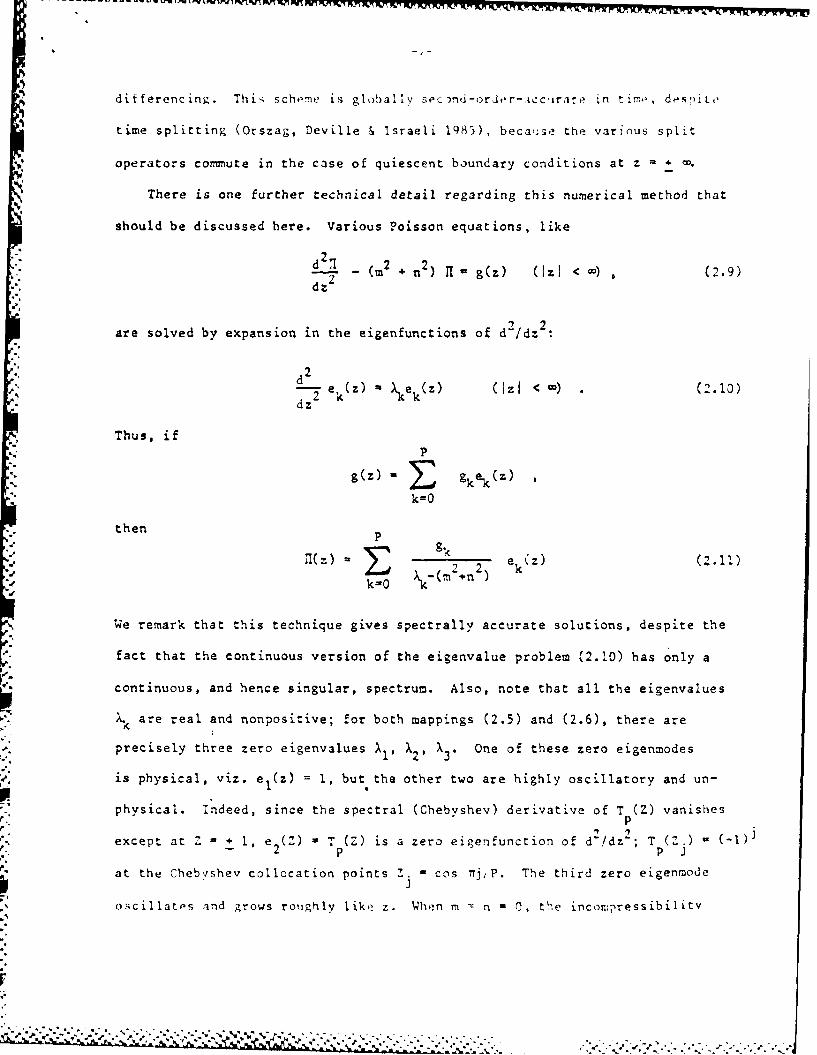
differencing. This schome is glohally sc )nd-orJer-accumrate in ti,,n, ds,)it

time splitting (Orszag, Deville & Israeli 1985), becau-se the various split

operators commute in the case of quiescent boundary conditions at z .

There is one further technical detail regarding this numerical method that

should be discussed here. Various Poisson equations, like

d.- (M2 + n2) II g(z) (ZI < ) (2.9)

dz 2

are solved by expansion in the eigenfunctions of d2/dz2:

d2

-e k(z) ke k (z) (OzI < =) (2.13)dz "

' Thus, if

g(z) =E gkek(z)k=0

then

11(z) e (z) (2.11)Lj 22 k". k=0 k - ( n )

We remark that this technique gives spectrally accurate solutions, despite the

fact that the continuous version of the eigenvalue problem (2.10) has only a

continuous, and hence singular, spectrum. Also, note that all the eigenvalues

>, are real and nonpositive; for both mappings (2.5) and (2.6), there are

precisely three zero eigenvalues X,, X X3" One of these zero eigenmodes1'2' 3-

is physical, viz. eI(z) = 1, but the other two are highly oscillatory and un-

physical. Indeed, since the spectral (Chebyshev) derivative of T (Z) vanishesp

except at Z i, e 2(Z) T (Z) is a zero eigenfunction of d /dz ; T (Z.)2 p p .

at the Chebvshev collocation points Z. - cos ?TTiP. The third zero eigenmode

oscillatos and grows roughly like z. When in - 0, the incopressibilitv

.. .... '-S , *'-', , a ,. 'i, - p- .& _.. - .. , .' ,,..,.," . . .

Irv ON VW

WV

constraint (2.2) requires that this mode of the z-velecitv field vanish identi-

cally so there is no difficulty with the zero-pressure eigenvalues X1, 2 , X 3.

Comparisons of the behavior of linear Orr-Sommerfeld eigenmodes obtained

using mappings (2.5) and (2.6) show that (2.6) gives a superior representation

of these modes unless L is fine tuned, which is not convenient in the nonlinear

dynamic runs.t Some representative results are given in Table 1. Notice

that as a increases, the optimal choice of map scale '" decreases. Also,

notice that the accuracy of the eigenvalue is much more sensitive to L for the

hyperbolic tangent mapping (2.5) than for (2.6).

This nonlinear, time-dependent Navier-Stokes code has been tested for the

generalized Taylor-Green vortex flow (2.12) and also for linearized eigen-

*. function behavior, with satisfactory agreement being achieved with power series

*. in t (Brachet et al. 1983) and linear behavior, respectively.

The second code used in the simulations is similar to the one just

described, except that sine and cosine expansions in z were used instead of

Chebyshev polynomials (2.4). Thus, the transverse domain extent is finite,

and care must be taken to identify possible interference effects. Comparisons

with results from the first simulations as well as simulations performed on

varying size domains has verified that such effects are small for the cases

t here is one case in which it seems that the hyperbolic tangent mapping (2.5)is more convenient than the algebraic mapping (2.6). This flow is the gen-

eralized Taylor-Green vortex flow that develops from the initial conditions

u(x,y,z,4)) sin x cos vycosh" z

v(x,y,z,O) - cos x sin y/cosh z (.U)

w(xV,z,O) = 0

The evolution of this flow seems best studied, either by power series or ini-tial value methods, using (2.5) with - 1. The time evolution of this freeshear flow is remarkably similar to that of the periodic Tavlor-oreen vorte:-(Brocher, Meiron, Orszag, Nickel., Morf & Friscb 1983).

--

presented here. Aside from details of the 1n:1",,otput h,:.,rin; rui!'t",:iA

the size of the arrays used in the computations, the basic code structure is

similar to that described in Orszag & Pao (1974).

3. Two-dimensional instabilities

In this and the following sections, results are reported for the evolution

of initial velocity fields of the form

1.

v(xy1Z,0) 0 0(Z) x + Re A10V10(z)e ) A (z)e

ia(x )+ity ](3.1)

where e .s the phase shift between the fundamental and subharnonic modes, and

is the corresponding phase shift of the spanwise mode. The laminar mean

profile is assumed to be U0 (z) - U 0 tanh z/6i, an approximation to the mixing

layer profile, and v..(z) is normalized so that max v. .z)l I. Here, 6. is

the initial mean vorticity thickness.

The initial functions v..(z) are normally chosen as the most unstable

eigenfunctions of the linear Orr-Sommerfeld equation for the appropriate wave-

numbers given in (3.1) (Michalke 1964).t In this representation, A10 is

the amplitude of the fundamental two-dimensional component, A1/2'D is the

amplitude of its subharmonic or pairing node, and A is the amplitude of the

primary three-dimensional wave with a spanwise wavelength equal to that of the

tlhe Reynolds numbers of the flows discussed below, while modest, are much

greater than that of the onset of linear instability (Rcrit "4), so thateven the linear modes are effectively inviscid. In this case, damped modes

1%may lie only in the continuous spectrum (Drazin & Reid 1981) and so aresingular. Whenever equation (3.1) calls for such a singular contribution tothe initial condition (3.1), we choose instead the flow component wn-of thOe fundamental mode (with uu, ,'nd Vnm dtermined 5y intompres;in itv)

.. ... ... .. . '

- in-

* fundamental two-dimension il mode. Tim;e is nndirmensinal izpd by U / and

space scales by 6.. The initial co..itions are typically chosen so that

A 1 1 2,0 , All << A 0 , and A - 0.25. The Reynolds number for the undisturbed

flow is R - Uo6i/v.

In the absence of subharmonic and three-dimensional perturbations

(A1/2,0 a All - 0), the two-dimensionally perturbed flow quickly saturates to a

quasi-steady state. In figure 1, a plot is given of the time evolution of the

two-dimensional disturbance energy E 0(t) for various initial amplitudes

A 0. The value for c is taken to be 0.4446, which is the wavenumber

corresponding to the largest growth rate predicted by linear theory (Michalke

1964). [The range of inviscidly unstable wavenumbers for the tanh z profile

is 0 < C < 1.1 Here

E (t) I J n (z,t)I dz (3.2)

• where p

V (zt) u(m,n,p,t) T (Z) (3.3)

pa0

and u is defined by (2.4). It is apparent that E. saturates into a finite-

amplitude vortical state on a time scale of order 10. The independence of the

peak saturation amplitude to the initial excitation amplitude except for every

high initialtamplitudes, which is evident in figure 1, has also been observed

experimentally by Freymuth (1966). If we define the growth rate 3 as

( (dE/dt)i(ZE) , 3.4)

then for linear disturbances of the form

' a = ekp(.)ei CQ(x-ct) ] .5

A.

VN

-Nl-

we have 0 a c . The peak growth rate of the most unstable linear node

(a = 0.4446) is 0 = 0.19. Our growth rates, which are given later in the tox:,

should be divided by a factor of 2 for comparison with the linear results for

oc. given by Michalke (1964) to reflect the different choice of U0 .

Figure 2 is a plot of the instantaneous spanwise vorticity distribution in

the developed two-dimensional flow for one of the runs shown in figure 1. Note

that while rollup is occurring by t 0 8, in the absence of a subharmonic mode,

A 1/2 0, pairing does not take place, and the flow evolves into the nonlinear,

quasi-equilibrium state shown in figure 2b. This absence of pairing is analo-

gous to that artificially induced by upstream forcing in experiments by Miksad

*(1972), Hussain & Zaman (1978), Oster & Wygnanski (1982), Ho & Huang (1982) and

others. In these experiments, the forced mode is amplified without also ampli-

fying its subharmonic. Thus, rollup of the forced mode is achieved without

pairing, creating a region in the flow characterized by large-scale, spanwise-

coherent, nonpairing modes. This produces countergradient momentum fluxes,

interruption in the growth of the mixing layer thickness, and a reversal in the

sign of the Reynolds stresses (Riley & Metcalfe 1980). That these phenomena

are also observed experimentally makes this nonlinear, quasi-equilibrium state

of interest in analyzing the physics of the laboratory flows.

The saturated two-dimensional flow state discussed above can be unstable to

subharmonic ?erturbations, A in (3.1), for suitable a (Kelly 1967). In1/2,0

figure 3, we plot the evolution of the subharmonic perturbation energies

E (t) as well as the fundaenta I two-dimensional energy E (t). Here we1/2,0 .10

choose A 0.25 and A 3x10 . In figure 3, the phase difference 9

between the two modes is ir/2a, so that pairing occurs. Values of 6 other than

integral multiples of 7 result in pairing, while pairinr is temporarily in hih-

ited when 0 is near NT, with N an integer. The cases 7 'N ar an)alc.ls,o

%1

. . . . . . . .

resulting in the "shredding interaction" ePt:ma> et al. 197-,) which is rar,..v

seen experimentally.t This subharnonic instabi'itv of tie saturated two-

dimensional vortical states is inviscid in character, as its growth rate asymp-

totically approaches a finite limit as R increases. The growth rate a1/2, 0

of the amplitude of the subharmonic mode is quite significant; at R a 200,

a1/2,0 = 0.1 when a - 0.4 while a112,0 t 0.2 for C = 0.8. These are not signi-

ficantly different from the corresponding linear inviscid growth rates of

Orr-Soumerfeld modes (Michalke 1964), which are a /2,0 = 0.14 and 0.19,

respectively.

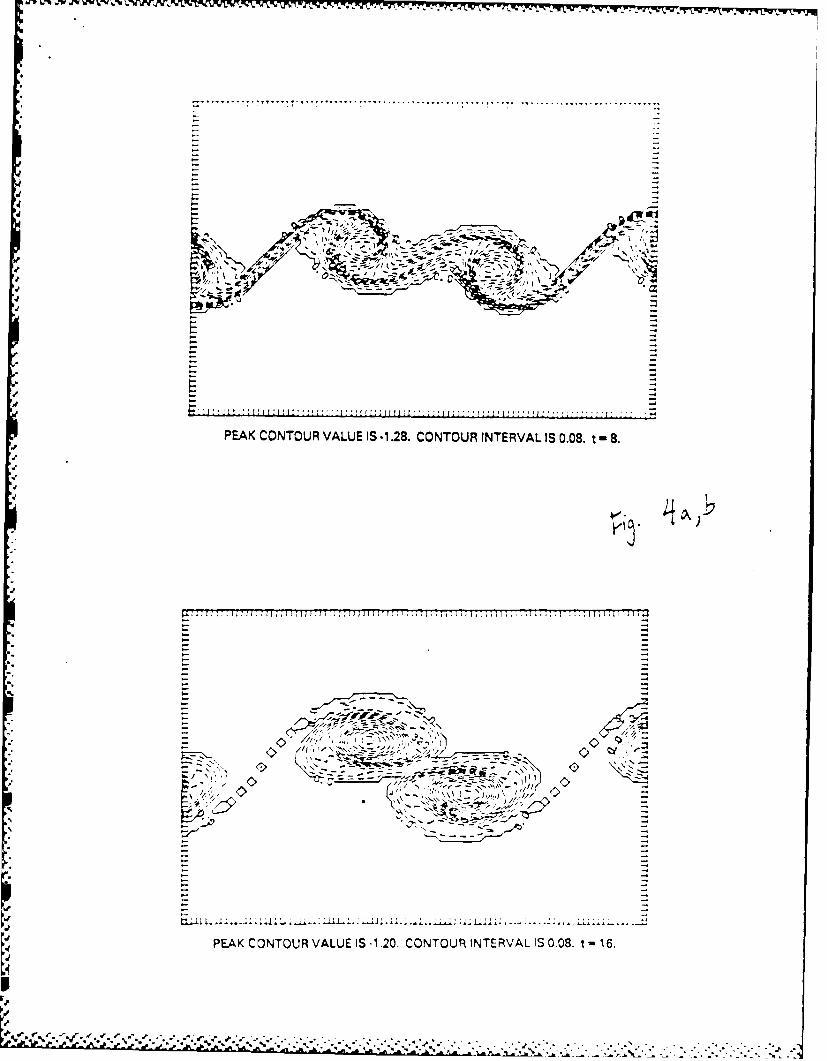
The evolution of the spanwise vorticity distribution during pairing insta-

bility is shown in the contour plots in figure 4 (from Riley & Metcalfe 1981).

There is strong similarity between these figures and flow visualizations of

mixing layers, such as those of Winant & Browand (1974). Note that in two

spatial dimensions, the lines of constant vorticity act as fluid markers much

like the dye used in experiments. The evolution of the pairing process is

strongly dependent on the relative initial amplitudes of the unstable modes.

When A 1 /2,0 = A1 0 , the fundamental mode rolls up first due to its higher

growth rate and shorter saturation time scale. The subharmonic continues grow-

ing after the fundamental saturates, during which time the vortex cores gener-

ated by the rollup of the fundamental are merged into t1e subharmonic core. In

this simulation (figure 4), the subharmonic -ode AI/ 2 , will become sat:ratel

after about t - 24, since there is no second subharmonic mode (A ,) wI:h1/4,0

which it can pair.

t See Rilev & Metcalfe (1980) or io & luerre pi..., p. 3 2) for additi naplots and a more detailed discussiin of ptiase diff,:rences.

'p .-'" - - - - - ' 3 i.i'. ,. , o -. , - , :. ./ _ ' . .. ?.-.N ... ,...-.,. ., ,-, . . . ,

-13-

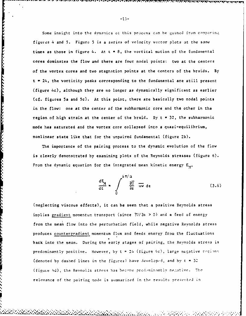
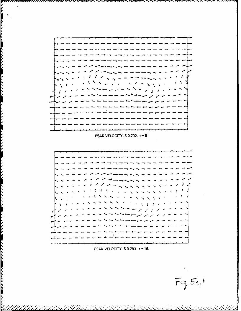
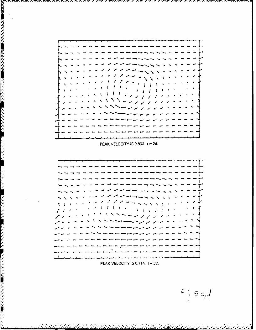
Some insight into the dynamics ot this process can be gained from cnmparin

figures 4 and 5. Figure 5 is a series of velocity vector plots at the same

times as those in figure 4. At t a 8, the vortical motion of the fundamental

cores dominates the flow and there are four nodal points: two at the centers

of the vortex cores and two stagnation points at the centers of the braids. By

t - 24, the vorticity peaks corresponding to the fundamental are still present

(figure 4c), although they are no longer as dynamically significant as earlier

(cf. figures 5a and 5c). At this point, there are basically two nodal points

in the flow: one at the center of the subharmonic core and the other in the

region of high strain at the center of the braid. By t - 32, the subharmonic

mode has saturated and the vortex core collapsed into a quasi-equilibrium,

nonlinear state like that for the unpaired fundamental (figure 2b).

The importance of the pairing process to the dynamic evolution of the flow

is clearly demonstrated by examining plots of the Reynolds stresses (figure 6).

From the dynamic equation for the integrated mean kinetic energy EM,

4 r/ adE.

au uw dz (3.6)

0

(neglecting viscous effects), it can be seen that a positive Reynolds stress

implies gradient momentum transport (since 2U/3z > 0) and a feed of energy

from the mean flow into the perturbation field, while negative Reynolds stress

produces countergradient momentum flux and feeds energy from the fluctuations

back into the mean. During the early stages of pairing, the Reynolds stress is

predominantly positive. However, by t = 24 (figure 6c), large negative recins

(denoted by dashed lines in the figures) have developed, and by t - 32

(figuie 6d), the Revnolds stress has bec'm-e preJominintlv ne,-ative. The

relevance of the pairing mode is sutmmarized in th. results presented in

-+ _ t , ,, ,, _', .v , •". .. . .- , . .....-. . - .... ,-.-.--. .- .

-14-

figure tre. Without the subharmonic pairinA mode, the Revnoldq stress changes

sign by t = 16. With the subharmonic present, however, the net Reynolds stress

is still positive at t - 16. Thus, the suppression of pairing, whether caused

by forcing, as in laboratory experiments (Hussain & Zaman 1978; Oster &

Wygnanski 1982; Ho & Huang 1982). or by eliminating the subharmonic mode, as in

the numerical simulations, is associated with a reversal in the sign of the

Reynolds stress.

This phenomenon is apparent in figure 3, in which the energy in the funda-

mental, E10 , reaches saturation by about t - 10. At this point, the Reynolds

stress changes sign, and a countergradient momentum flux develops. In the

absence of other disturbances, this flow will then evolve into an oscillatory

state characterized by an alternating energy exchange between the mean flow and

the perturbation fields.

In terms of turbulence models, the presence of pairing is essential to

maintain the positivity of transport coefficients (such as eddy viscosity).

Since the eddy viscosity, Ve , is related to the Reynolds stress by

eddVeddy

it follows that suppression of the pairing corresponds to a negative eddy

viscosity. This suggests that accurate simulations of flows with inhibited

pairing may require the direct calculation of large-scale structures.

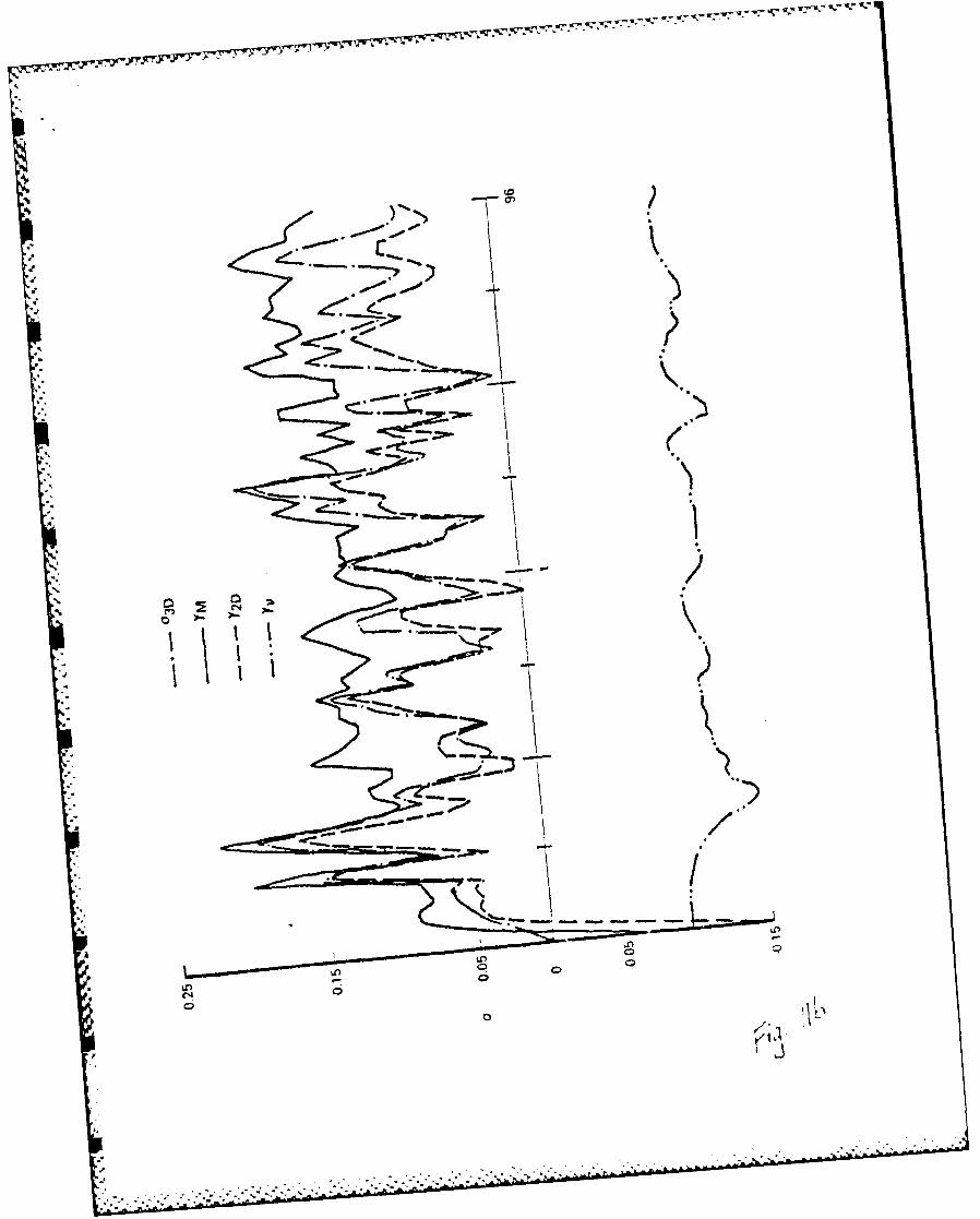
The energetics of the pairing instability is revealing. Energy transfers

to and from the subharmonic mode may be decomposed as

dE

I d t 0

-- , "

S.

wht!re v, involv3 the nonlinear interaction of the subharm.onic mode with Ph,.

mean flow, yD the nonlinear interaction of the subharmonic mode and all

other two-dimensional modes, and Y the viscous dissipation of pairing energy.

Here TM and Y2D involve sums over nonlinear terms in the Navier-Stokes

equations but are unaffected by pressure; y is proportional to the enstrophy

in the subharmonic mode. In figure 7, a plot is given of these transfer terms

as a function of time. It appears that the subharmonic mode extracts most of

its energy from the mean flow and that there is little net energy transfer

between it and the fundamental mode. In addition, its average growth rate

differs little from that in the absence of the fundamental, which is a = 0.14.

Thus, the presence of the saturated two-dimensional fundamental does not turn

off the subharmonic mode, and the growth rate of this latter mode is close to

that of the fundamental two-dimensional instability. These results imply that

even a small subharmonic perturbation will quickly achieve finite amplitude

after the fundamental mode saturates, unless the amplitude of the fundamental

is artificially amplified by forcing. In this simulation, the subharmoni= mode

saturates at t = 90 at which time the growth rate becomes negative. It

should be noted here that in attempting to compare these results for growth

rates of the fundamental and subhar=onic modes with experiments, it is neces-

sary to account for the dispersion of the subharmonic modes (cf., for example,

figure 2b in Ho & Huerre 1984), which is present in the spatially growing but

not in the temporally growing mixing layer. Also, in comparing these growth

rates with those predicted by lUnear theory, the growth of momentum thickness

of the mixing layer over the course of the simulation should be taken into

consideration.

0

Corcos & Sherman (1984) find that the presence of the fundamental id~ihlts

the subharmonic growth, while Pierrehumbert & Wi-nall (1982) find an enhance-

ment of growth. We find that the growth rate of the subharmonic is modulated

with a period related to the oscillation time scale of the nonlinear, quasi-

equilibrium fundamental mode. However, the net effect on the growth of the

subharmonic due to the fundamental is to decrease C1/20 slightly, from

about 0.16 to 0.14. While these conclusions do agree with those obtained by

Kelly (1967) using perturbation theory, they show that the effect is quite

small.

4. Three-dimensional instabilities

The saturated two-dimensional flow is also subject to three-dimensional

instabilities. While the laminar mean flow is inviscidly unstable only for

2 + ( 2 < 1, the finite-amplitude two-dimensional flow can be unstable for

%large 5 at high Reynolds numbers. :n figure 8, we plot the average three-

dimensional growth rate C3D versus 3 of the three-dimensional disturbance

eriergy,

E3D - Zm!(t) .

m

for various Reynolds numbers when C - 0.4 for a three-dimensional linear

perturbation to a saturated, two-.1mensiznal quas.-equilibrium flow. Analysis

of these results suggests the conjectures that, as R increases, for a fixed 3,C3D approaches a finite lm=.': " o the secondary instability d~scussed is

inviscid in character) an' that the instahil:." turns off for

crit

I..'f --, € ,., ,-.- ,-, I , % - ,f % . . -'.. . . , . . , . , . , , . . . , . . . .

A4 " TM Pr 9 .9. V W W W~W V%-W -CW V-T V

-17-

Although the mean flow tanh z is both viscously and invscidly stable for

3 > I, the saturated, two-dimensional disturbed flow is strongly unstable at

these scales, with disturbances growing at rates near those of the inviscid

two-dimensional fundamental instability, as shown in figure 9. When the two-

dimensional modes saturate, the three-dimensional modes can achieve finite

amplitudes on convective time scales and thereby modify significantly the later

evolution of the flow.

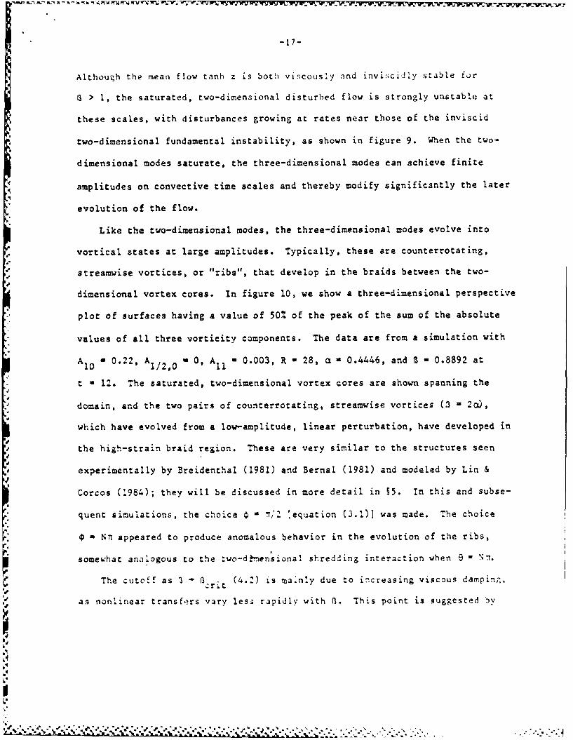
Like the two-dimensional modes, the three-dimensional modes evolve into

vortical states at large amplitudes. Typically, these are counterrotating,

streamwise vortices, or "ribs", that develop in the braids between the two-

dimensional vortex cores. In figure 10, we show a three-dimensional perspective

plot of surfaces having a value of 50% of the peak of the sum of the absolute

values of all three vorticity components. The data are from a simulation with

A10 - 0.22, A1/2,0 " 0, A11 - 0.003, R - 28, a a 0.4446, and a - 0.8892 at

t - 12. The saturated, two-dimensional vortex cores are shown spanning the

- domain, and the two pairs of counterrotating, streamwise vortices (3 - 2a- ,

which have evolved from a low-amplitude, linear perturbation, have developed in

the high-strain braid region. These are very similar to the structures seen

experimentally by Breidenthal (1981) and Bernal (1981) and modeled by Lin &

Corcos (1984); they will be discussed in more detail in §5. In this and subse-

quent simulations, the choice T /'-' 'equation (3.1)] was made. The choice

a N1 appeared to produce anomalous behavior in the evolution of the ribs,

somewhat analogous to the two-dkmensional shredding interaction when e = N .

The cutoff as 3 - ri (4.2) is mainly due to increasing viscous damping,

as nonlinear transfers vary less rapidly with R. This point is suggested by

A

.. . . .. . .. . . . . . .. . . . . .

[?r' 1-7 P- 1% W. A 1 N -. A; W % U RV

the results plotted in figure 11, where we plot the con ribitions to the growth

rate U3D3DE3

1 d 3D "YM * "2D * YV (4.3)2E 3D dt 3

Here Y. involves the nonlinear interaction of the three-dimensional and mean

flows, and (2D the interaction of the three-dimensional and two-dimensional

energy. The jitter in the plots is due to numerical inaccuracy in the evalua-

tion of the nonlinear transfer terms, so only the trends in the data should be

considered significant. It is suggested from the data in figure lla that, for

3 < acrit , yV and 2D << yM asymptotically so that the three-dimensional mode

derives its energy from the mean flow with the two-dimensional disturbance

acting as a catalyst for this transfer.

On the other hand, the results plotted in figure llb show that when

a= crit' YV is quite significant. The three-dimensional instability seems to

be turned off at a large cross-stream wavenumber a by increased dissipation

rather than by any significant qualitative change in nonlinear transfers from

the mean and two-dimensional components.

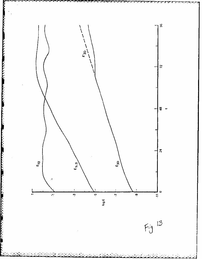
The nature of the competition between two-dimensional pairing and three-

dimensional instability is illustrated by the results plotted in figures 12 and

13. In both figures, we have plotted the results of runs with R - 400, a a 0.4,

and B a 0.2. Figure 12 shows the evolution of the instabilities when the

initial three-dimensional perturbation is much larger than the subharmonic

mode. In this case, the pairing instability is nearly unaffected by the three-

dimensional instability before finite amplitudes are reazhed. In figure 13,

the initial conditions are chosen so that the subhar-inin mode perturbation is

much larger than that of the threc-dimen~ioni1 pert-riation; it seems that tho

.,* *.. . . *.. * *.I -

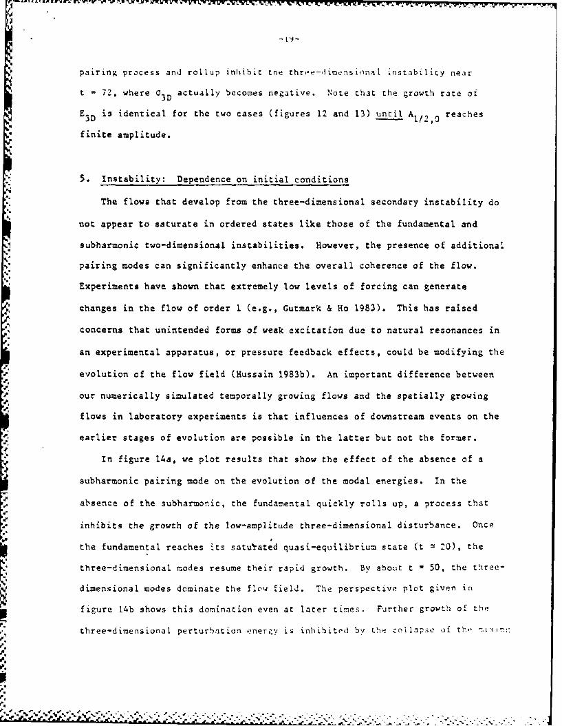
pairing process and rollup inhibit the three-dimensional instability near

t = 72, where C3D actually becomes negative. Note that the growth rate of

E3D is identical for the two cases (figures 12 and 13) until A 1/2,0 reaches

finite amplitude.

5. Instability: Dependence on initial conditions

The flows that develop from the three-dimensional secondary instability do

not appear to saturate in ordered states like those of the fundamental and

subharmonic two-dimensional instabilities. However, the presence of additional

pairing modes can significantly enhance the overall coherence of the flow.

Experiments have shown that extremely low levels of forcing can generate

changes in the flow of order I (e.g., Gutmark & Ho 1983). This has raised

concerns that unintended forms of weak excitation due to natural resonances in

an experimental apparatus, or pressure feedback effects, could be modifying the

evolution of the flow field (Hussain 1983b). An important difference between

our numerically simulated temporally growing flows and the spatially growing

flows in laboratory experiments is that influences of downstream events on the

earlier stages of evolution are possible in the latter but not the former.

In figure 14a, we plot results that show the effect of the absence of a

subharmonic pairing mode on the evolution of the modal energies. In the

absence of the subharmonic, the fundamental quickly rolls up, a process that

.- inhibits the growth of the low-amplitude three-dimensional disturbance. Once

the fundamental reaches its saturated quasi-equilibrium state (t = 20), the

three-dimensional modes resume their rapid growth. By about t - 50, the three-

dimensional modes dominate the flow field. The perspective plot given in

figure l4b shows this domination even at later times. Further growth of the

three-dimensional perturbation energy is inhibited by the colapse of th' :

0. .0..

01.

layer due to the absence of the subhar-onic. With the subhi-1mIonic present, the

evolution of the three-dimensional modes is dramatically different. The

results plotted in figure 14c are from a simulation identical to the previous

one except for the inclusion of the subharmonic mode. The zhree-dimensional

modal growth (at amplitudes in the linear range) is now slowed both by the

fundamental rollup (t 2 5-10) and by the subharmonic pairing (t = 20-35).

Thus, the flow is more coherent than in the absence of the subharmonic (compare

figures 14b and 14d). Once the subharmonic reaches its saturated state

(t = 35), the three-dimensional growth rate increases substantially.

As was pointed out in 14, the two-dimensional and three-dimensional

unstable modes grow at very similar rates when all disturbance amplitudes are

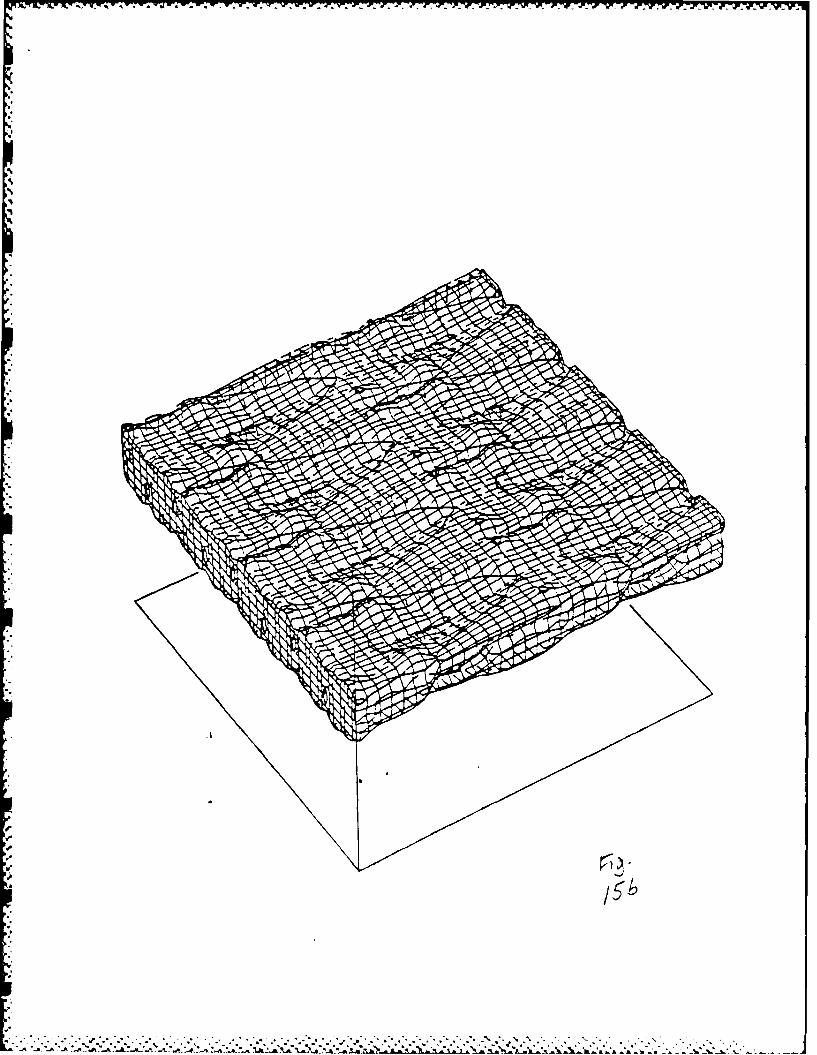
in the linear range. In figure 15, we plot the results of a simulation in

which both fundamental and three-dimensional modes were introduced at approxi-

mately equal amplitudes, well down into the linear range. In this case, the

three-dimensional mode disrupts the rollup and saturation of the fundamental

mode, so that its peak amplitude is an order of magnitude smaller than without

the three-dimensional mode present. As shown in figure 15b, the presence of

the large three-dimensional instability substantially reduces the spanwise

coherence.

To determine whether the model used to initiate the three-dimensional

instabilities in the simulations described thus far was realistic, we performed

several simulations initialized with a broad range of three-dimensional modes.

We used an uncorrelated, random-phase velocity field having a Gaussian-shaped

energy spectrum. This field was convolved with a function so that the relative

turbulence intensity levels were consistent with those of experimental mixing

layer data. However, the initial peak intensity leve. was about 3 orders of

I' " ' '"'"'" % "' '"' "-- " ." ---- - - '- ." .... -, ",

_ W %. 1 Awl W1~ PM " ~ I RW1U.L AMn . - V Nl17 V

magnitude below the experimental values, so the initial disturbance growth wa-

in the linear regime.

In figure 16a, we plot the evolution of the flow field with broad-band

initial excitation. Neither fundamental nor subharmonic two-dimensional linear

eigenfunction modes were explicitly included in the initial conditions, although

there was energy in the corresponding wavenumbers defined by the random ini-

tialization process. Nonetheless, E10 and E1 /2, 0 grow very rapidly initially,

with al 10 0.11 and a 1/2,0 a 0.13 at t = 10 (compared with a 1/2,0 - 0.19 and

10 a 0.14 for linear inviscid modes). EZ, which is the energy in all velocity

components not having ky 0, has a growth rate of a 3D 0.12 at t - 10. When

the modal components of EZ reach finite amplitude (at t 35), C3 D decreases

sharply and the flow field is characterized by a chaotic, turbulent-like velo-

city field in the center of the mixing layer (figure 16b). The flow remains in

this chaotic state until the subharmonic reaches nonlinear amplitude and begins

to roll up. As the subharmonic reaches its saturation amplitude (t = 90),

the nature of the three-dimensional velocity field evolves from a highly chaotic

state to one with coherent, large-scale structures (compare figures 16b and

16c), although C3D remains approximately constant. Thus, there is a complex

interaction between the two- and three-dimensional instabilities. The coherent,

two-dimensional modes significantly enhance the growth of the mixing layer

thickness, creating a larger region for the ultimate expansion of three-

dimensional instabilities. During their rollup and pairing processes, however,

the coherent, two-dimensional modes tend to reduce significantly the growth

rates of the low-amplitude three-dimensional modes.

The inhibition of the three-dimensional modal growth rate by the rollup and

pairing of the two-dimensional modes is a function of both the amplitude ani

% F '****.*.*.t. . *U--

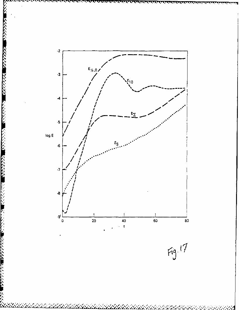
the wavenimber of the threc-dimensional modes. Fo)r low-amplitude tlree-

dimensional modes, in the linear range, coherent rollup or pairing can actually

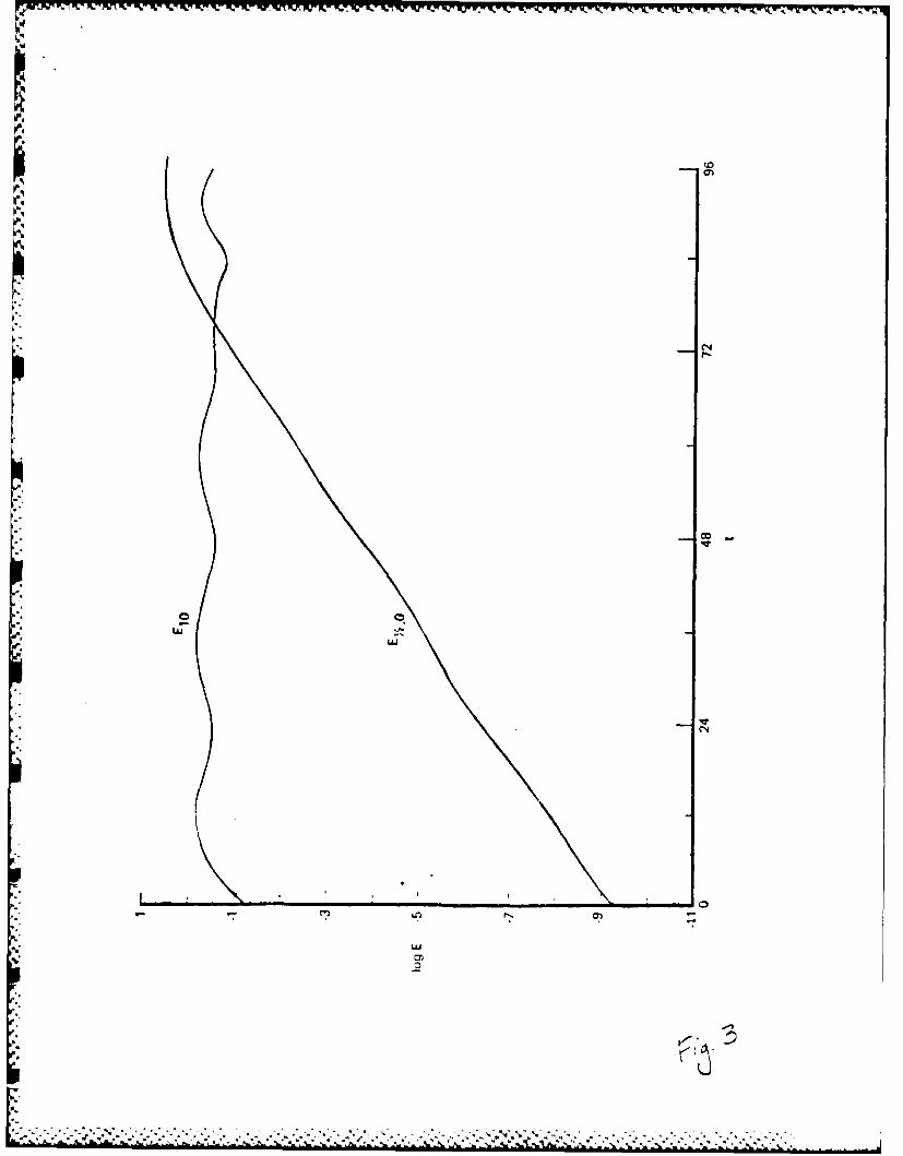
be stabilizing. In figure 17, we plot the evolution of the modal energies as

functions of time for a simulation with the same initial conditions as in

figure 16 but with A - 0.0014. As seen in this figure, when the funda-1l/2,0

mental and subharmonic reach nonlinear amplitudes (t = 25), the three-

dimensional growth is stopped completely. At higher three-dimensional modal

amplitudes, however, the rollup may have little or no effect on C3D" For

example, in figure 16a, a3 D changes very little in the presence of the

saturating subharmonic between t - 60 and 100. During the three-dimensional

stabilization shown in figure 17, the low 3 modes continue to grow while the

high a modes decay. This is not unreasonable, since as the scale of the mixing

layer grows due to the two-dimensional pairing, the relative scale of the

spanwise instability also changes. As shown in figure 8 for three-dimensional

perturbations to two-dimensional saturated modes, T3D depends strongly on

3. A similar effect is seen for E Z in the nonlinear range in figure 16a.

This would perhaps be manifest in the formation of larger ribs after the pair-

ing of the two-dimensional modes. One mechanism that may have a significant

influence on the suppression of the three-dimensional modal growth is the

temporal variation of the strain field in the braids between the coherent,

two-dimensional vortices. In the early stages of rollup, a very high strain

develops in the braids. This has a tendency to stretch the ribs, intensifying

the streamwise vorticity. As the two-dimensional modes approach saturation,

however, the strain rate decreases substantialv, so that this vortex stretch-

ing mechanism is weakened.

-e a r'

SWA

-23-

6. The secondarv instabi I itv in a tur-tzl,,nt flow

We have performed high-resolution (64x64x64 mode) simulations of a fully

turbulent mixing layer, and it is instructive to relate the evolution of these

flows to the class of instabilities discussed so far. These simulations were

performed on a computational domain sufficiently large to allow two complete

pairings (periodicity length 871/a). The initialization procedure was

similar to that discussed in §5, but the amplitudes of the initial fields were

higher. Details of the numerics are given in Riley, Metcalfe & Orszag (1985).

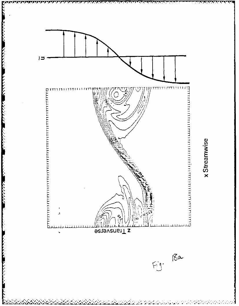
The spanwise vorticity field after two complete pairings shows clear

evidence of large-scale structures (see figures 18a and b). A comparison of

the vorticity plots at two different spanwise locations indicates a strong

spanwise coherence for this particular realization, although details of the

structures are different. As previously noted, the secondary instabilities in

the mixing layer flow are characterized by streamwise, counterrotating vortices

that tend to form in the braids. Figure 19 is a contour plot of wo in a

plane at the middle of the mixing layer (z - 0). The solid and dashed lines

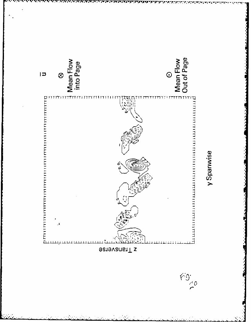
indicate positive and negative vorticity, respectively. Figure 20 is a similar

plot at a streamwise location B/4 from the left boundary in figure 19. These

two plots clearly indicate the presence of such vortices, although they are

irregularly spaced.

One of the best laboratory visualizations of coherent, three-dimensional

structures in a turbulent mixing layer was performed by Bernal & Roshko (cf.

Bernal 1981). Using laser fluorescein dye techniques, they were able to

illuminate the flow at a fixed streamwise locat~on. The most striking

characteristic of these photographs is the appearance of mushroom-shaped

features on the braids between the two-dimensional vortex cores (figure 21a).

We have been able to simulate this technique 'hv enplcving a numerical cod-

... ...,*.... -... ,... .... *'. .,.*-.... . .. ....... -* .. . .

. W-r-.

developed to study a chemically reacting mixing laver (Riley et al. W5) in

which the advection diff'usion equations for a binary ch.ical reaction are solved

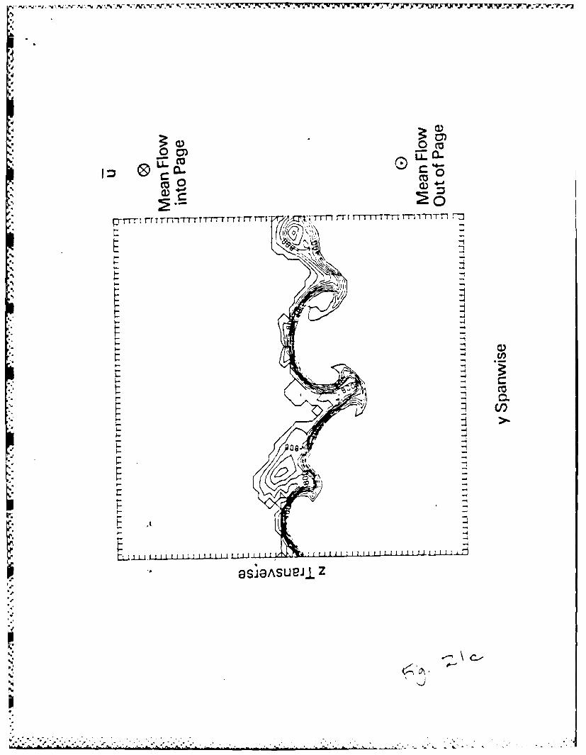
along with the Navier-Stokes equations. Figure 21b is a contour plot of the

concentration of one of the chemical species on the same plane as in figure 20,

and figure 21c corresponds to the concentration of the other chemical species.

A comparison of figures 20 and 21b shows that the counterrotating vortex pairs

tend to pump fluid through the braid between their cores, increasing the reac-

tion surface area and creating the mushroom shaped structures in the flame

front, which is defined by the region of overlap between figures 21b and 21c.

Such features were also noted in the model proposed by Lin & Corcos (198).

The structure of the streamwise, counterrotating vortex tubes is made

clearer by isolating the streamwise vorticity component of the flow. Figure 22

is a three-dimensional perspective plot of surfaces at which 1W I equals

50% of its peak value. This figure was from the same realization and at the

same time as figures 18-21. The large-scale, spanwise-coherent structures do

nor show up in this plot since they consist mainly of spanwise vorticity,

wy . Comparison with figures 18a and 18b shows that the ribs do form on the

braid between the large-scale two-dimensional vortex cores. This structure is

consistent with the model proposed by Bernal (1981) although the irregular

spacing of the ribs suggests that the modification of this model proposed by

'ussain (1983a) is more realistic. The effect of increased coherence of the

two-dimensional pairing modes on the rib structure is shown in figure 23, which

is from a simulation like the prtvious one but to which two-dimensional modes

have been added in the initial conditions: A,, M 0.1, A. ,2,0 = 0.06,

A 0.025 [equation (3.1)]. The resulting ribs are more coherent and* 1/4,0

Tmore aligned in the streamwise direction. As was the case with the simulation

in figure 11, the preqence of the pairing mode tends t, increase the coh'rence

O f the three-dimensional prti:rbatijn field.

_ - . ,- ** . . . ,1 . ...

The extreme sensitivity of the ribs to the initial or upstrea:n flow

conditions makes direct quantitative comparisons between the simulations and

laboratory experiments difficult. In the simulations we have performed so far,

there have been significant variations in the amplitudes and spanwise spacing

of the ribs. Likewise, in the experiments of Bernal (1981), there was

substantial scatter in the measurements of the rib spacing. In addition, he

found that the spanwise position of the ribs appeared to be related to

disturbances originating upstream in the settling chamber. Our stability

analysis (figure 8) has shown that there is a broad range of spanwise

wavenumbers that are unstable. Some representative values for the simulation

shown in figures 18-22 are as follows: the peak spanwise vorticity normalized

by the peak mean velocity gradient is about 2, while the peak streamwise

vorticity is slightly higher, about 3. The spanwise vorticity amplitudes are

consistent with filtered experimental data (Metcalfe, Hussain & Xenon 1985),

while the streamwise vorticity amplitudes are somewhat higher than in other

runs. The rib spacing (estimated from figure 19) is about the same as the

wavelength of the most unstable fundamental two-dimensional mode. This is in

the range of values reported by Bernal (1981). A more detailed analysis of

these simulations, using experimental data to refine these comparisons, is now

in progress.

7. Discussion

We have shown that small-scale three-dimensional instabilities like those

previously studied by Orszag & Patera (1980, 1983) and P errehumbert & Widnall

(1982) exist in free shear flows and that these instabilities persist to

moderately low Reynolds nur-'bers. It n s w clear that t-,.s' nodes can be

reF-onsible for the initial dev#-lop:,rnto. tYr,',,-d> ,'n . n itv in th.,se sh, l:

f lows. The dynanics of thI~se thre9-d:-..,n.on, instab L es i smilar to

that of the three-dimensional instabilities r, wall-bounded shear flows. At

high amplitudes, these instabilities manifest themselves mainly as counter-

rotating, streamwise vortices, or ribs, that form on the braids between the

spanwise-coherent, two-dimensional pairing modes; they are responsible for the

generation of the mushroom-shaped features seen in laboratory experimental

visualizations (Bernal 1981). While the instabilities share some features of a

classical inflectional instability, including phase locking with the funda-

mental vortex, inflectional instabilities are preferentially two-dimensional,

whereas the present instabilities are not.

The rollup and pairing of the two-dimensional modes has a stabilizing

effect on the higher spanwise modes and on the overall three-dimensional growth

rate when the amplitude of the three-dimensional modes is small, while the

absence of pairing (saturation) can enhance the three-dimensional growth rate.

However, in the absence of pairing or rollup, the three-dimensional instabil-

ities can reach a chaotic, saturated state from which significant further

growth is not possible without additional pairing. The suppression of the

low-amplitude three-dimensional instabilities by pairing could explain the

strong two-dimensionality of the flow near the splitter plate in many labora-

tory experiments. Once the three-dimensional modes reach a finite amplitude

and/or the Reynolds number increases with do%.;strean distance, tne growth

suppression effect is reduced, and the flow beco=es mcre three-dimensional.

Mixing can be enhanced initially by ccherent fzrcing of the mixin; Laver to

saturation (Hussain & Zaman 1978; Oster & Wv nanski L382; Ho & Huang 19S2),

which will enhance the growth of the three-diensional modes to a chaotic

state. But this is done at the expense of redicin; t-e growth of the lx i :

laver momentun thickness, which is due tr~ari> to the a :rerss Th,

ao

-27-

-he maximizatinn o pr duct for-iatiur. in a rca-t i xi'g l.'-.r i l r, .

balancing the increases in the flame front area -enorated by the chaotic

three-dimensional flow with the increases due to the more rapid mixing layer

growth caused by the presence of additional pairing modes.

The results of these simulations suggest that, with respect to the grzwth

of three-dimensional disturbances, there are several important flow states

possible in an evolving mixing layer. First, there is pairing and rollup of

the two-dimensional modes, which is characterized by a suppression of low-

amplitude three-dimensional modal growth at low Reynolds numbers. Second,

there is the saturated, two-dimensional, quasi-equilibrium, non-pairing state,

which is highly unstable to three-dimensional perturbations. Finally, there

are chaotic, three-dimensional states characterized by a lack of spanwise

coherence from which only moderate three-dimensioral growth can occur. It is

from these states that more rapidly growing, large-scale, two-dimensional modes

can eventually emerge and reorganize the flow in a manner consistent with that

suggested by Staquet & Lesieur C1986).

It seems that the mechanics of transition in the free shear flows studied

here may, in a sense, be rather more complicated than in the case of wail-

bounded shear flows. In the latter case, linear instabilities are often

viscously driven and, therefore, weak, so they cannot be directly responsible

for the rapid distortions characteristic of transition. On the otner hai,

free shear flows are subject to a variety of inviscid instabilities, so t"cre

may be many.paths to turbulence: We have shown that the choice cf ;at. s in an,.

individual flow may depend in the results of ccrnetiticn between ftinda 7!-t:

subharmonic, and three-dimensional instabilities, all of whic , are on.':t

driven and, therefore, strong with c'pa:a: e r rat,- . Thus, th, . -

tion of frie, !,near [!ows in tra- uit;onal r' . . , s '

past hi.tory of the flow, including ":.e rdi.e a u cnp tin',

modes, the mechanism of their generaton, an] ::.e extenal environment in w

the flow is embedded.

I

T'"

a-

..

u'.

Bernal, L. P. 1981 The coherent structure of turbulent mixing layers. I.

Similarity of the primary vortex structure. 1I. Secondary strea-wise

vortex structure. Ph.D. thesis, Calif. Inst. Technol., Pasadena.

Bernal, L. P., Breidenthal, R. E. Brown, G. L., Konrad, J. H. & Roshko, A.

1979 On the development of three dimensional small scales in turbulent

mixing layers. In Proc. 2nd Int. Svmp. on Turbulent Shear Flows, Imperial

College, London.

Brachet, M. E., Meiron, D. I., Orszag, S. A., Nickel, B. G., Morf, R. H. &

Frisch, U. 1983 Small-scale structure of the Taylor-Green vortex. J.

Fluid Mech. _30, 411-452.

Breidenthal, R. 1981 Structure in turbulent mixing layers and wakes using a

chemical reaction. J. Fluid Mech. 109, 1-24.

Browand, F. K. & Troutt, T. 1980 A note on spanwise structure in the two-

dimensional mixing layer. 3. Fluid Mech. 97, 771-781.

Brown, G. L. & Roshko, A. 1974 On density effects and large structures in

turbulent mixing layers. J. Fluid Mech. 64, 775-816.

Busse, F. H. & Clever, R. M. 1979 Instabilities of convection rolls in a

fluid of moderate Prandtl number. J. Fluid Mech. 91, 319-335.

Collins, D. A. 1982 A numerical study of the stability of a s:ratified

mixing layer. Ph.D. Thesis, Department of Mathematics, McGill U'niv.,

Montreal.

Corcos, G. M. & Sherman, F. S. 1984 The mixirg layer: deterministic models

of a turbulent flow. Part l. ntroduction and the two-dimensional flow.

° Fluid X-c . Y119, 2q-65.

I.. % - . . % , ° . o . - • . , . . o . - . - . . .. . ..

r.cs, .. M. & Lin, S. J. 198. h. m i., I .r d t er-ii,. tic ,lels 1 :

turbulent flow. Part 2. The otgn t - e ::! e-' 1-:e:1iona notion. .

fluid Mech. 13_, 67-95.

Drazin, P. G. & Reid, W. H. 1981 Iivdrodva-.,ic ?tabiitv, Cambridge

University Press.

Freymuth, P. 1966 On transition in a separated laminar boundary laver. J.

Fluid Mech. 25, 683-704.

Gutmark, E. & Ho, C.-M. 1983 Preferred modes and the spreading rates of

jets. Phys. Fluids 25, 2932-2938.

*Ho, C.-M. & Huang, L.-S. 1982 Subharmonics and vortex merging in mixing

layers. 3. Fluid Mech. 119, 443-473.

Ho, C.-M. & Huerre, P. 1984 Perturbed free shear layers. Ann. Rev. Fluid

Mech. 16, 365-424.

Ho, C. H. & Nosseir, N. S. 1981 Dynamics of an impinging jet. Part 1. -he

feedback phenomenon. J. Fluid Mech. 105, ll -l42.

Hussain, A. K. M. F. 1983a Turbulence and :hactic Phenomena in Fluids,

edited by T. Tatsumi, 453. North-Holland.

-" Hussain, A. K. M. F. 1983b Coherent structures--realiy and myth. Phys.

Fluids 26 (10), 2816-2850.

Hussain, A. K. H. F. & Zaman, K. B. H. Q. 1978 The free shear layer tone

phenomernn and probe interference. F-.id Mec". _, 3.9-383.

Kelly, R. E. 1967 On the stability of an inviccid shear layer which is

periodic in space and time.- 3. Fluid Meh. _', 657-.

• Lin, S. J. & Corcos, G. M. 1984 The mixin; aver: deternistic m,'deo s a

turbulent flow. Part 3. The e".ec: of :Ian strain 7n the dynamics -

streamwise vortices. J. Fluid MIoc. 14., :3o-l.

• II

a: . . ° . ° -• • . ° . . ..-.. . .

-3'

XetcaIf e, R. W. , ltuss.tin, A. K. M. F. & S , on . li, C. ,t striture

in a turbulent mixing layer: A comparison between direct numerical

simulations and experiments. To appear in Proc. 5th Svmn. 7urbulent Shpir

Flows. Springer-Verlag.

Michalke, A. 1964 On the inviscid instability of the hyperbolic tangent

velocity profile. J. Fluid Mech. 19, 543-556.

Mi.ksad, R. W. 1972 Experiments on the nonlinear stages of free shear layer

transition. J. Fluid Mech. 56, 695-719.

Orszag, S. A. & Pao, Y. 1974 Numerical computation of turbulent shear flows.

,n Advances in Geoph.sics, Vol. 18A, 225-236. Academic.

Orszag, S. A. & Patera, A. T. 1980 Subcritical transition to turbulence in

plane channel flows. Phvs. Rev. Lett. 45, 989.

Orszag, S. A. & Patera, A. T. 1983 Secondary instability of wall-bounded

shear flows. J. Fluid Mech. 128, 347-385.

0rszag, S. A., Deviile, M. 0. & Israeli, M. 1986 Splitting methods for

incompressible flow problems. '. Comp. Phys., 7o be published.

Oster, D. & Wygnanski, I. 1982 The forced mixing layer between parallel

streams. 7. Fluid Mechi. 123, 91-130.

?atnaik, P. C., Sherman, F. S. & Corcos, G. M. 1976 A numerical simulati:n

of Kelvin-emi'oltz waves of finite amplitude. J. Fluid Mech. 73, 215-'_42.

Pierrenumbert, R. T. & Widnall, S. E. 1982 The twa- an, three-dimensiona.

instabilities if a spatially periodic shear layer. :. Fluid Mech. 2l4,

Riley, .. J.. & ,zafe, R. W. '1932 Direct nu-ericil sin-ila:ion of a

...... ,irb,:er .m.i:g. laver. A.AA .aper.,.-.....

IV LI'.

Riley, J. J., Met lf:e, R. W. , Orsza. , S. A... 1 6 ' hirec_ numerical

simulations of chemically reacting turbulent mixing layers. Accepted for

publication in Phys. Fluids.

Staquet, C. & Lesieur, M. 1986 The mixing layer and its coherence examined

from the point of view of two-dimensional turbulence. Submitted to J.

Fluid Mech., September 1985.

Stuart, J. T. 1967 On finite amplitude oscillations in laminar mixing layers.

J. Fluid Mech. 29, 417-440.

Winant, C. D. & Browand, F. K. 1974 Vortex pairing: the mechanism of turbu-

lent mixing-layer growth at moderate Reynolds number. J. Fluid Mech. 63,

237-255.

Wygnanski, I., Oster, D., Fiedler, H. & Dziomba, B. 1979 On the perseverance

of a quasi-two-dimensional eddy-structure in a turbulent mixing layer. J.

Fluid ' ech. 93, 325-335.

.9

-9.

-3

Table I. ;rnwth rates ( rn c) 3f the orr-So-"., orfr'I,! eigenfunctionsfor the mixing layer 110(z) - Ut tanh (z/'i)t

x-wavenumber ca

0.25 0.5 0.75

Number of Chebyshev Polynomials (P4i)

L 17 33 65 17 33 65 17 33 65

Hyperbolic Map (2.5)

0.5 1.534 1.375 1.238 0.579 0.501 0.457 0.160 0.150 0.150

1 0.959 0.820 0.746 0.383 0.360 0.351 0.141 0.138 0.1372 0.635 0.614 0.605 0.344 0.342 0.342 0.137 0.137 0.137

4 0.612 0.598 0.597 0.324 0.342 0.342 0.041 0.136 0.137

8 0.539 0.597 0.597 0.115 0.322 0.342 S 0.045 0.136

16 0.202 0.526 0.596 Stt S 0.321 S S 0.046

Algebraic Map (2.6)

0.5 0.699 0.588 0.599 0.345 0.346 0.342 0.131 0.138 0.1371 0.591 0.599 0.597 0.344 0.342 0.342 0.137 0.137 0.1372 0.600 0.597 0.597 0.342 0.342 0.342 0.136 0.137 0.1374 0.597 0.597 0.597 0.325 0.342 0.342 0.371 0.136 0.137

8 0.542 0.597 0.597 0.009 0.322 0.342 S 0.043 0.!36

T Here the Reynolds number is U06i/v a 100 and the eigenvalue is the complexwave speed c for a temporal mode of the form (z)ei _(xct). For the most

rapidly growing mode listed here, Re(c) - 0.

tt S indicates that all modes are stable with the indicated parameter values.

.1

"w ' . .[ . .' V . :" . . . . ; . ' . . , , . . - . - , - - - . . - . . . . . . - . - . .

* Figure Captions

FIGURE 1. A plot of E 1(t) versus t for runs with A1/2,0 Al z 0 and

A10 0 0.5, 0.25, 0.125, 0.01. Here the Reynolds number is

R -00, the spectral cutoffs in (2.4) are M - 8, N - 1, P - 32

(resolution 8xlx32 with no subharmonic modes), the x-wavenumber is

a - 0.4, and the time step is At = 0.02. Note that the flow

saturates into a vortical state nearly independent of the initial

perturbation. Before such saturation occurs, the perturbation

grows linearly like an Orr-Sommerfeld eigenfunction.

FIGURE 2. Contour plots of spanwise (y) vorticity for the mixing layer at

t * 8 and t - 32 with R - 83, A 1/2, 0 - 0, A10 = 0.2,

M - P - 64, and N = 1.

FIGURE 3. Plots 3f the evolution of E10 (t) and the two-dimensional

subharmonic mode energy E1/2,0(t). Here R " 400, A1 0 " 0.25,3xi-4A 1 3x10 , M - 8, N a 1, P - 32, a - 0.5, At - 0.02,/2,0

and - ir/2a (phase difference between the two modes).

FIGURE 4. Spanwise vorticity contours at t - 0, 8, 16, and 24, during a

vortex pairing run with R a 83, A1 0 0 0.20, A 1 /2,0 = 0.14,

M - 64, N - 1, P = 64 (resolution 64xlx64 ), a - 0.4446,

At 0.05, and e - It/2a.

FIGURE 5. Velocity vector plots of the vortex pairing run shown in figure 4.

FIGURE 6. (a - d) Plots of the Reynolds stress at different times for the

runs with both fundamental and subharmonic present (figure 4).

(e) A plot of the Reynolds stress with and without pairing at

different times.

IJ'." '2 ;.',''.'.". %.. '' . ". ' .. ". . ., ,: , . . . . . . . . . . .

F-j .Fr j V - 77- .7777 27 - if ,7'" -

-35-

FIGURE 7. A plot of the components yM' 2D' * 'see (3.3)1 of

the growth rate G1/2,0 of the subnarmonic node amplitud.e as

functions of time for a run with R 200, A 0 , 0.25,-5A 0 3xlO , M - 16, N 1 1, P 32, a = 0.43, and

% Lt - 0.01.

FIGURE 8. A plot of the computed three-dimensional growth rate a3D [see

(4.3)] as a function of the spanwise wavenumber a for various

Reynolds numbers. Here a a 0.4.

FIGURE 9. A plot of the computed subharmonic growth rate '1/2,0 and

three-dimensional growth rate "3D as a function of c at

R = 400 and 3 - 0.8.

FIGURE 10. A three-dimensional perspective plot of surfaces having a value

equal to 50% of the peak of the sum of the absolute values of all

three vorticity components for a run with R = 56 (at t a 12),

M N - P - 64, a - 0.4446, Lt - 0.05, A 1 0.22, 2,0 ,

A1 - 0.003, a - 0.8892 at t - 12.

FIGURE 11. A plot of the components M Y2D m [see (4.32] of the

three-dimensional growth rate a 3D as functions of time for

R - 400, a = 0.4, A = 0.25, A 11 = 10*10 1

(a) B , 4.

(b) 3 6.

FIGURE 12. A plot of the evolution of the energies E1 0 , E/ 1 :0 E3D

versus t for a run with R = 400, a = 0.4, .3 0.2, M 8, N " 4

P - 32, and initial conditions A1 0 M 0.25, A1 /2,0 3x1A 10- 3 . The thrqe-dimensional mode initially dominates thesubharmonic mode.

A160.Tetredinnin1md ntal oiae h

F GU'RE 13. Sam as figure 12, exce p t ti thie ini tia con itions ire

A, 0.25, A -4x o. A .3.3x1 C, li,, t D

from figure 12. Note that the linear growth OL the three-dimensional

mode is stopped when the subharmonic reaches a nonlinear amplitude.

FIGURE 14. (a) A plot of the evolution of the modal energies as functions of

time. ES a E 0 + E + E21, i.e., the three lowest spanwise

modes with the same x-wavelength as the fundamental. R a 100,

a a 0.4446, A1 0 0 0.22, A 1 2 0 - 0, and A 1 = 10-

(b) A three-dimensional perspective plot of the vorticity field as

in figure 10 at t = 96.

(c) Same as figure 14a but A/2 0.14.

(d) Same as figure 14b but A1 12 .0 - 0.14.

FIGURE 15. (a) Same as figure 14a but A 10- 3 .

10,J~(b) Sarx e as figure 14b but A1 0 10 - at t ,:48.

FIGURE 16. (a) A plot of the evolution of the modal energies as functions of

time. Er - energy in all modes with k # 0. R - 100. Randomy

noise initial field with peak rms velocity 0.01.

(b) A three-dimensional perspective plot of the vorticity field as

in figure 10 at t - 48.

(c) Same as figure 16b but at t - 96.

FIG'~ 17. A plot of the evolution of the modal energies as functions of tine.

Z -energy in all modes with k y 0. R = 100,

a - 0.4446, A1 0 = 0, A1 /2, = 0.0014, and All i0.

FIGURE 18. Spanwise vorticity at y - 4r/a (figure 18a) and 67/a (figure l3b).

The computational doiain'size B is 8r/ct. R - 154 and t = 72.

.anlo. noise initial field with peak rms velocity 0.13. Tho

ir.itial Reynolds number is R 28.

-37-

FIGURE 1'). Strea:nwise vor' icity at z ) r th.2 sa.. run a in rigg'.r.! 13.

FIGURE 20. Strearawise vorticity at x 2T/a for the same run as in

figure 18.

FIGURE 21. (a) Laser sheet/fluorescein dye visualization of the braid of a

(b) Contour plot of the species concentration field at the same

time and location as in figure 20.

(c) Contour plot of the second species concentration field at the

same time and location as in figure 21b.

FIGURE 22. Three-dimensional perspective plot of surfaces at which Iw Ix

equals 50% of its peak value for the same run as in figure 18.

FIGURE 23. Plot of iw I as in figure 22 but for a simulation to which

two-dimensional modes have been added in the initial conditions:

A1 0 -0.1, A1 12,0 -0.06, and A /4, 0 0.025 [equation (3.1)].

V.,

4

v-.'%. ,.%.-..% .-

-p % " ': ' " " ' ' ' ' '' " ' ." " " " : • , ' . J : ' ', ' . ' _ e ' . - - : . - - , .., ,

0~ 0N .- NUT)L

44

..... ~ ..... . ., V

PEAK CONTOUR VALUE IS -. 12. CONTOUR INTERVAL IS 0.07. t-3.

7%7~~ ILI %'.W P--PAp L ~l

'4)

C.'

CN

ui0- - C., I-0.cm

- ~-~-~--~

)-. ~ ~- ~-'..,,

I1

1 -I' I! I

PEAK CONTOUR VALUE IS .1.28. CONTOUR INTERVAL IS 0.08. t -8.

I

I

d

- =

1,1,~.-.

c< ~

,,

N N

E '2:------------------ - - .., I'-- ~ ---z-~---~~ ~ l~I

* N'~"' ~ /1/f K>K ~~

H -.

PEAK CONTOUR VALUE IS *1 .20. CONTOUR INTERVAL IS 0.08. - 16.

I.9

* . * ,*~

-rTT.7M 7T," -1 '71

I IA.

5. I '. >

'I -zz

IIIII H IIII II I j 1 111

PEAK ~ ~ ~~ W COTU AUIS-.2 OTU NEVLI .7 4

I ~ ~ ~ ~ ~ ~ ~ ~ ' III -II T M T IIIi1 1M M ~ ;IiIiIII : 1 1 1 1 1 1 1 1 sI

i - Z

~ .. j\ .--

PEAK CONTOUR VALUE IS-i.1. CONTOUR INTERVAL s 0.07. t 32.

41 = +~- -" - ,- • , -" -v ;+ :i . I- i-...l- - 9 - -

'U. -• " " /" "'-- "" - - ""

i ' \ % I I i - \ \ \:

- - " -a - -,, - - - -

" ..

.

p,,-

--------------------- - - ----- - ----------------

- - - - -|' - v T- , v v - T - v

• , v ! t -,..-

.. , - - , - . ' . • ~• " " / / / l \ \ " a

I,, ~ ' \ \/ '~ .,

PEAK VELOCITY IS 0.800. t ==24.

o .,

-- - -- - - -

CONTOURS ARE FROM -0.032 to 0.104. CONTOUR INTERVAL IS 0.008. t -8.

CONTOURS ARE FROM -0.05 TO 0.11. CONTOUR INTERVAL IS 0.01. t -16.

N0

/o f

2 0La

.. .. 6A.

CONTOURS ARE FROM -0082 TO 0016 CONTOUR INTERVALZ 0.001 2

- (P)

00

cciSS38iS0 0CN3

.d.

1.a -

* -a'

a..

-- I

.1

I.>-a-..--.

0 C 0- a- 0 C.

0 0 0 0 9

0

* U

d

-d

4C.

. -o

-St

00

0 -4

r'4 CD 0

rF-2- W ----- O 'W. -. -

>IeaL~co

9w l z

rAJ N-

I I ,C

ii°

rno~ I,-A-.----

C--% k*-' ,* )

* ~

~

(A

'N.

* - -w

)

I,

0

0 0

-p........................

* * .*- . "-.- '. N.

a - - - -

v.tJ

CDm

- CD C~1 W - -S

0 I *

-a

S.

A

m m m

0 0

.1

A

a.

-- '---VAk.k fg'~ai

CN

I I

10

Lfl 1%

wj

N1%

.2

'. / \,.

.3 N1

..ES:

Iog E 4

N •.

.5 ...

i-6

o"-6 80 100.'0 20 40 6

.

p,

1:

'..-..

* *. *~ 4 - - -

U

d

S

.4

'U

'C.

C..

C., 1'Cf.

Cf.

C.C,

C,

Ca.

'C.'

a a A

-1

lo E~

/

0 * 20 4%0 0810

. / -,, \.I \ .. ''9' I /'

' , .4

'I .'4... . . S....r-

• • , . ,°-. • , . ... , .% - • -E -* "

U

A

A,,

A,

A,

'A

A-,

., WA*~ - - - -

E 1

S-5

J..

"$ -3

0400

/:

5'. / ..

.5 /o°

U,. I.-/"

l o g E 6 -- I .

-. / ./ "

.7 -/ /

020 40 60 80 10t

5-..- - -.. ' - .",,,,' ... ,. . ,.- -,,-,. ... .t,- -,.,- .,., - -. .- -..-. .. .. . .-. -... .... .-

- ' 4' a . - - -'

9~

a.

S.

'9

V.

-9.-

U, -2

.3 #

.0. .

log E

-9

0 25 50 75 100

- -.. .- ~ - - .' - - - - - -

4

-t

-'S

5%

5~

-'5

-p

.*%.**.. '...~*., ''U*'*'*~ -. -.-. 5-a-.

~ ~ (s~..L..A. .. k~A... - ~2. .. .. .. -.

n.1 1

-2

/". -3 -- / /#".,

/ . ,io -3I

/ ' /% %

a .. ." '-500,

logE ..

/"I .ES '-6 I . .

-7 I"

26

.. I*. I

III

/I

0 20 40 60 80t

.4,

AW.7 - W. i/I

ITT iii i ir V- T 7,- -rT I-

I- CA

Ec

OSGAue. z~

pr11 r I -- -h TMlr 7 -!T ~ 77 T1 -T T- - -

4E

Cr iTFT rr~1Tr7

r ~rn ur rnrSAr

/Z I li lt

OSJOASeJ.L2

/

C' -K..~? ,

A - / /,* / - A- \ JIJ/~ ~ 1 j'~ 0 -:1

V.-

/ / Ky)-, '1

-- 0.0

I-

C,- (J2

dNp a

I-' /~ .~, .-

cC'-.-, E:1: C,

*~'r ~,

) $1,111-asIMued9 ~?-, 0 2 /

I"' I.' - -'I / I - - - -

- I.-~ Hi .- ~ -4

/ -~ - g

\\. I,,. Cl 10

A

A5

5%

ci

'isI",

S.

.5.

'.5

MC LL C-

®cQ

-~ 01

-4

GS9A4e. Z

* U~ M. JL ~ ~ ~-. w~; ~-. ~ ~ 'r~-~ ~ .? ~.?' ~) - -' - .. - - .

I..I

I

~.1

~.1

* .-~

,-~ ,,~.

*~5*.* *S- *I~~' *-* ~ ... -.. .. -. -* 55 5~ *** *.*..5. ~.***..,..... .. *-**5-S*- ~=*%.~.**~5*~- -.. * * ~ S..~

- "-a t~e -a ~. S Ar ~

c - '

CC

c~cu

I 'V TLL lmr fit if mi- 11. rrj jLl- 1, r1r "'r FT1~ T r

9-. A~~.Z

b4

000

7rrIT- T T rTFF=T T= 7T TTT T7T1 TIT r? rrTTrrlIl TTn rFl

t

.Poe

aS9SL Z/

5%

5.

'S.

5.

5'

'S

.5

S..

.5'P

5'

.5'

-- 5

.1SS

K p

0 -

d~z-. -

5%

Iwx~

7

S.'5~

S.

S'S

§ *§5§~j;i. *j§ §X~1~-. 5-S.'. ' '.

- -~ .~ ~'-.'

S

Iw~

S

* N

C

Y~ V I U - * .

4* .-. .- .. *- .. 5*' .-- -.. S

5 '5 5 5 .5S*~** **~5* ***5 *.~5 * * -

4 . * S * * S5~55~ *~ * S -

5J5 5. . ~555* - - . . .